Photon generation from vacuum in nondegenerate cavities with regular and random periodic displacements of boundaries

Abstract

We study the influence of fluctuations in periodic motion of boundaries of an ideal three-dimensional cavity on the rate of photon generation from vacuum due to the nonstationary Casimir effect.

PACS: 42.50.Lc; 46.40.Ff; 72.80.Ng; 03.65.-w

Key words: Dynamical Casimir effect; Periodically moving boundary; Fluctuations; Transfer matrix; Disordered chain

1 Introduction

Among many interesting classical and quantum phenomena in cavities with moving boundaries, the effect of photon creation from the vacuum seems to be the most impressive. The first rough (although not always quite correct) estimations were made by several authors in Refs. [1, 2, 3, 4, 5, 6]. More detailed and consistent studies performed for the past decade in the frameworks of different approaches [7, 8, 9, 10, 11, 12, 13, 14, 15, 16, 17, 18, 19, 20, 21, 22, 23, 24, 25, 26, 27, 28, 29, 30, 31] (for other references see review [32]) predicted, indeed, an exponential growth of the field energy in the case of periodic motion and under the resonance conditions, when the walls vibrate at the frequency which is a multiple of the unperturbed field eigenfrequency.

Now, an experimental verification of theoretical predictions becomes a difficult but realizable task. An idea which seems to be the most realistic at the moment is to realize an effective moving mirror by means of periodic creation of a conducting layer from a semiconductor film posed on the surface of the cavity wall and irradiated by powerful laser impulses [33]. Different prototypes of this idea were discussed in [34, 35], but not in a periodic regime (for other schemes see, e.g., [36, 37]; however, their realizations seem to be more difficult). The effective mirror scheme has several advantages over the primary idea of an acoustic excitation of harmonical surface vibrations of the wall [13].

The main of them is the removal of severe limitations on the maximal dimensionless amplitude of the displacement of the surface, which resulted from tremendous internal stresses inside the wall whose surface vibrates at the necessary frequency having an order of several GHz (or higher). In the effective mirror scheme, the maximal displacement of the boundary depends of the thickness of the semiconductor film and the laser power, and it can be made several orders of magnitude larger than the maximal displacements (not exceeding $10^{-8}\,$cm [13]) which could be achived in the scheme based on the acoustic excitation of the surface vibrations. As a consequence, one can diminish (in the same proportion) the number of oscillations of the boundary necessary to produce photons in the cavity, thus relaxing the requirements for the $Q$-factor of the cavity and the admissible detuning from the exact resonance [18, 19]. Another advantage is a possibility to use periodic pulses of arbitrary shape, whose period can be much longer than the period of oscillations of the chosen mode of electromagnetic field.

However, a practical realization of the scheme depends on its robustness against inevitable experimental imperfections, such as, e.g., nonexact periodicity of laser pulses (creating free carriers in the semiconductor layer) or fluctuations in their power. Therefore, the aim of our article is to give some estimations of possible deviations from ideal results caused by such imperfections.

2 Basic relations

The most part of theoretical studies on the nonstationary (dynamical) Casimir effect was performed within the framework of the model of a one-dimensional (Fabry–Perot) cavity with equidistant spectrum of unperturbed eigenfrequencies of the field, when all modes are coupled in the resonance case. However, in realistic three-dimensional cavities the spectrum is, as a rule, nonequidistant. This results in great simplifications in the resonant case, when periodic motion of the boundary excites only one resonant mode, whereas the response of all other modes can be neglected in the long-time limit [13]. Therefore, we confine ourselves here to this simplest case (interesting phenomena which could occur in cavities with few accidentally resonant modes, when the ratio of their unperturbed eigenfrequencies is integral number due to some additional symmetry, were considered recently in [25, 26, 29]).

In this case, as was shown in [13], the problem of photon generation in the selected mode is reduced to the problem of excitation of a quantum oscillator with a time dependent frequency $\omega(t)$, which is determined by the instantaneous geometry of the cavity. For example, in a rectangular cavity with fixed dimensions $L_{x},L_{y}$ and a variable dimension $L_{z}(t)$ we have

$$\omega(t)=\pi c\left[\frac{n_{x}^{2}}{L_{x}^{2}}+\frac{n_{y}^{2}}{L_{y}^{2}}+\frac{n_{z}^{2}}{L_{z}^{2}(t)}\right]^{1/2}.$$ (1)

For fifty years passed after the seminal paper by Husimi [38], this last problem was studied in detail in numerous publications (for reviews see, e.g., [39, 40]). It appears that all properties of the quantum oscillator are determined, as a matter of fact, by the fundamental set of solutions of the classical equation of motion

$$\ddot{x}+\omega^{2}(t)x=0.$$ (2)

Here we actually need only one consequence of the general theory, namely, that the mean number of quanta generated from the initial oscillator ground state due to the time dependence of frequency is given by the energy reflection coefficient from an effective “potential barrier” given by the function $\omega^{2}(t)$. More precisely, if $\omega(t)=\omega_{i}$ for $t\to-\infty$ and $\omega(t)=\omega_{f}$ for $t\to\infty$ (this means that the cavity wall is supposed to assume some fixed positions before and after the experiment), then one has to calculate the coefficients of the asymptotical form of the solutions to Eq. (2),

$$x(t\to\infty)=\omega_{f}^{-1/2}\left[\xi e^{i\omega_{f}t}+\eta e^{-i\omega_{f}t}\right],$$ (3)

satisfying the initial condition $x(t)=\omega_{i}^{-1/2}e^{i\omega_{i}t}$ for $t\to-\infty$. Due to the unitarity of evolution, these coefficients obey the identity

$$|\xi|^{2}-|\eta|^{2}=1.$$ (4)

The mean number of quanta for $t\to\infty$ can be expressed in terms of $\xi$ and $\eta$ as follows [6, 41],

$${\cal N}=|\eta|^{2}={R}/{T},$$ (5)

where $R\equiv|{\eta}/{\xi}|^{2}$ and $T\equiv 1-R\equiv|\xi|^{-2}$ can be interpreted as energy reflection and transmission coefficients from the effective potential barrier.

Eq. (5) shows that no photons can be created during a single pass of the wall from one position to another, because for monotonous functions $\omega(t)$ the reflection coefficient is limited by the Fresnel formula

$$R_{1}=\left(\frac{\omega_{i}-\omega_{f}}{\omega_{i}+\omega_{f}}\right)^{2}$$ (6)

corresponding to very rapid change of position (for the time much less than the period of field oscillations) [42]. Since real boundaries in laboratory experiments can only move with velocities much less than the speed of light, the process is almost adiabatic, and $R_{1}\ll 1$. However, it is well known that the reflection coefficient can be made very close to unity in the case of periodic variations of parameters due to interference effects.

For a periodic motion of the wall, the function $\omega^{2}(t)$ is also periodic. We assume that it has a form like that shown in Fig. 1. The most important assumption is that each “effective potential barrier” is well separated from the next one by some interval of time where $\omega=const$ (i.e., that the wall moves for some period of time, returns to its initial position, stays at this position for some time, and then repeats the cycle). Thus we exclude monochromatic oscillations of the boundary, which have been already studied in detail in [13].

Figure 1: A typical time dependence of the effective frequency.

In such a case, each “barrier” can be completely characterized by two complex amplitude reflection coefficients and two complex amplitude transmission coefficients, which connect the “plane waves” coming from the “left” and from the “right”. Namely, if some “barrier” begins at $t=0$ at terminates at $t=t_{*}$, then one can write two independent solutions of Eq. (2) outside the “barrier” as (hereafter we consider for simplicity the case of equal initial and final constant values of the frequency $\omega$)

$$x^{(-)}(t)=\left\{\begin{array}[]{ll}e^{i\omega t}+r^{(-)}e^{-i\omega t},&t<0\\ t^{(-)}e^{i\omega t},&t>t_{*}\end{array}\right.$$ (9)

$$x^{(+)}(t)=\left\{\begin{array}[]{ll}t^{(+)}e^{-i\omega t},&t<0\\ e^{-i\omega t}+r^{(+)}e^{i\omega t},&t>t_{*}\end{array}\right.$$ (12)

(We use the letter $t$ without supescripts to denote the time variable, whereas the same letter supplied with supescripts means the amplitude transmission coefficient; we hope this will not lead to a confusion.) The coefficients $r^{(\pm)}$ and $t^{(\pm)}$ are not independent, because equation (2) is invariant with respect to complex conjugation (the frequency $\omega(t)$ is real). The following relations hold (see, e.g., [43, 44]; the simplest way to obtain these relations is to calculate Wronskians for suitable pairs of independent solutions):

$$t^{(-)}=t^{(+)}\equiv t^{(\pm)},$$ (13)

$$r^{(-)}t^{(\pm)*}+r^{(+)*}t^{(\pm)}=0,$$ (14)

$$|r^{(-)}|^{2}+|t^{(-)}|^{2}=|r^{(+)}|^{2}+|t^{(+)}|^{2}=1.$$ (15)

Suppose now that we have several well separated “barriers”, the $n$th “barrier” (possessing coefficients $r_{n}^{(\pm)}$ and $t_{n}^{(\pm)}$ if it begins at $t=0$) being shifted in time by the value $t_{n-1}$ (with $t_{0}=0$) with respect to the beginning of the first one. Then one can combine the first $n$ barriers in a single effective barrier, characterized by the amplitude reflection and transmission coefficients $\rho_{n}^{(\pm)}$ and $\tau_{n}^{(\pm)}$. There are many different methods enabling to express these coefficients in terms of $r_{k}^{(\pm)}$ and $t_{k}^{(\pm)}$, $k=1,\ldots,n$: see, e.g., [45, 46] and references therein. We use the method of transfer matrix [6, 47, 48, 49, 50, 51, 52, 53] (see also [54] for historical review and [55, 56, 57] for the most recent applications).

Let us write the solutions to Eq. (2) after the $k$th barrier (in the region where $\omega(t)=\omega=const$) as

$$x^{(k)}(t)=a_{k}e^{i\omega t}+b_{k}e^{-i\omega t},$$ (16)

with suffix $0$ related to the solution before the first barrier. Evidently, every two sets of the nearest constant coefficients, $(a_{k-1},b_{k-1})$ and $(a_{k},b_{k})$, are related by means of a linear transformation

$$\left(\begin{array}[]{c}a_{k}\\ b_{k}\end{array}\right)=M_{k}\left(\begin{array}[]{c}a_{k-1}\\ b_{k-1}\end{array}\right).$$ (17)

Comparing Eqs. (16) and (17) with (9) and (12), and taking into account the identities (13)-(15), one can express the elements of matrix $M_{k}$ as follows:

$$M_{k}=\left\|\begin{array}[]{cc}f_{k}^{*}&-g_{k}^{*}\\ -g_{k}&f_{k}\end{array}\right\|,$$ (18)

where

$$f_{k}\equiv[t_{k}^{(\pm)}]^{-1},\quad g_{k}\equiv r_{k}^{(-)}/t_{k}^{(\pm)}.$$ (19)

Consequently, each matrix $M_{k}$ is unimodular:

$$\det M_{k}=|f_{k}|^{2}-|g_{k}|^{2}\equiv 1.$$ (20)

We shall use the notation

$${\cal M}_{n}=\left\|\begin{array}[]{cc}F_{n}^{*}&-G_{n}^{*}\\ -G_{n}&F_{n}\end{array}\right\|$$ (21)

for the total transfer matrix of $n$ barriers, shifted in time by $t_{k}$, $k=1,\ldots,n-1$, with respect to the initial instant $t=0$. Applying consecutively the transformations (17) with account of the phase shifts $\theta_{k}\equiv\omega t_{k}$ (with $\theta_{0}=0$), one can obtain the following matrix formula:

$${\cal M}_{n}=\Phi_{n\!-\!1}M_{n}\Phi_{n\!-\!1}^{\dagger}\Phi_{n\!-\!2}M_{n\!-\!1}\cdots\Phi_{1}M_{2}\Phi_{1}^{\dagger}M_{1},$$ (22)

where

$$\Phi_{k}\equiv\left\|\begin{array}[]{cc}\exp(-i\theta_{k})&0\\ 0&\exp(i\theta_{k})\end{array}\right\|.$$ (23)

Eq. (22) is equivalent to the recursive relations

$${\cal M}_{k}=\Phi_{k-1}M_{k}\Phi_{k-1}^{\dagger}{\cal M}_{k-1},$$ (24)

$$F_{k}=g_{k}G_{k-1}^{*}e^{2i\theta_{k-1}}+f_{k}F_{k-1},$$ (25)

$$G_{k}=g_{k}F_{k-1}^{*}e^{2i\theta_{k-1}}+f_{k}G_{k-1},$$ (26)

where $F_{0}=1$ and $G_{0}=0$. One can verify that Eqs. (25) and (26) preserve the identities

$$|F_{k}|^{2}-|G_{k}|^{2}\equiv 1.$$ (27)

The total mean number of quanta (5) created after $n$ impulses is nothing but

$${\cal N}_{n}\equiv|G_{n}|^{2}.$$ (28)

The coefficients $\rho_{n}$ and $\tau_{n}$ themselves obey the nonlinear recurrence relations

$$\rho_{n}=\frac{\rho_{n-1}+r_{n}s_{n-1}\exp(2i\theta_{n-1})}{1+\rho_{n-1}^{*}r_{n}s_{n-1}\exp(2i\theta_{n-1})},$$ (29)

$$\tau_{n}=\frac{\tau_{n-1}t_{n}^{(\pm)}}{1+\rho_{n-1}^{*}r_{n}s_{n-1}\exp(2i\theta_{n-1})},$$ (30)

where $s_{n}\equiv{\tau_{n}}/{\tau_{n}^{*}}$, $\rho_{1}=r_{1}^{(-)}$, $\tau_{1}=t_{1}^{(\pm)}$.

3 Strictly periodic motion of boundaries

Formula (22) becomes especially useful in the case of strictly periodic motion of boundaries, when all one-barrier matrices $M_{k}$ coincide with $M_{1}$, and $\Phi_{k}\equiv\Phi_{1}^{k}$:

$${\cal M}_{n}=\Phi_{1}^{n}(\Phi_{1}^{\dagger}M_{1})^{n}.$$ (31)

Obviously, the matrix $\Phi_{1}^{\dagger}M_{1}$ is unimodular, as well as matrix $M_{1}$. Therefore, we can use the well-known formula for the powers of any two-dimensional unimodular matrix $S$ (see, e.g., [48, 54]):

$$S^{n}=U_{n-1}(z)S-U_{n-2}(z)E,\quad z\equiv\frac{1}{2}\mbox{Tr}S,$$ (32)

where $E$ means the unit matrix and $U_{n}(z)$ is the Tchebyshev polynomial of the second kind.

In the case discussed, introducing the new parameter $\nu$ according to the relations (hereafter $\theta\equiv\theta_{1}$, $g\equiv g_{1}$, $f\equiv f_{1}$)

$$z=\mbox{Re}\left(fe^{-i\theta}\right)=\pm\cosh\nu,$$ (33)

and using the hyperbolic representation of the Tchebyshev polynomial

$$U_{n}(\cosh\nu)\equiv\frac{\sinh[(n+1)\nu]}{\sinh(\nu)},$$ (34)

we arrive at the following explicit expressions for the elements of matrix ${\cal M}_{n}$ (for simplicity, we suppose that the sign of variable $z$ in Eq. (33) is positive; this sign does not affect the final result (37) for the number of created photons):

$$G_{n}=g\,\frac{\sinh(n\nu)}{\sinh(\nu)}e^{i\theta(n-1)},$$ (35)

$$F_{n}=f\,\frac{\sinh(n\nu)}{\sinh(\nu)}e^{i\theta(n-1)}-\frac{\sinh[(n-1)\nu]}{\sinh(\nu)}e^{i\theta n}.$$ (36)

Consequently, the number of created photons after $n$ impulses equals

$${\cal N}_{n}=|g|^{2}\frac{\sinh^{2}(n\nu)}{\sinh^{2}(\nu)}.$$ (37)

The generation of photons is possible provided parameter $\nu$ is real, i.e.,

$$|f|\,|\cos(\varphi-\theta)|>1,\quad f\equiv|f|e^{\varphi}.$$ (38)

Since $|f|>1$, one has to ajust the phase shift $\theta$ to the phase of the inverse transmission coefficient $\varphi$. The maximal effect is achieved for

$$\theta=\theta_{res}\equiv\varphi+\pi m$$ (39)

(with $m$ an integer). This is equivalent to the following relation between the periodicity of impulses $T=\theta/\omega$, the period of the electromagnetic field oscillations in the mode concerned $T_{0}=2\pi/\omega$ and the phase $\varphi$:

$$T=\frac{T_{0}}{2}\left(m+{\varphi}/{\pi}\right).$$ (40)

In particular, for nonmonochromatic oscillations of the boundary, the field mode can be excited not only under the condition of the parametric resonance $T=T_{0}/2$, but the period of motion of the boundary can be greater than the period of field oscillations. This fact may be important for possible experimental arrangements.

Under the condition (40), $\cosh(\nu)=|f|$ and $\sinh(\nu)=|g|$, so that

$${\cal N}_{n}^{(res)}\! = \!\!\sinh^{2}\left(n\nu\right)$$

$$\equiv \!\!\frac{1}{4}\left[\left(\frac{1\!+\!|r|}{1\!-\!|r|}\right)^{n/2}-\left(\frac{1\!-\!|r|}{1\!+\!|r|}\right)^{n/2}\right]^{2},$$

where $r\equiv r_{1}^{(-)}$ is the amplitude reflection coefficient from each barrier (remember the relations (19) between different coefficients). If $|r|\ll 1$, then one can replace $\nu$ by $|r|$. Then for $n|r|>1$ we have

$${\cal N}_{n}^{(res)}\approx\frac{1}{4}\exp(2n|r|).$$ (42)

In the case of a harmonically oscillating boundary near parametric resonance,

$$\omega(t)=\omega_{0}\left[1+2\varepsilon\sin(\Omega t)\right],\quad\Omega=2(\omega_{0}+\delta)$$ (43)

($\omega_{0}$ is the unperturbed field eigenfrequency, and $\Omega$ is the frequency of the wall vibrations), the number of quanta created from vacuum is given by the expression [18] (under the conditions $|\delta|\ll\omega_{0}$ and $|\varepsilon|\ll 1$)

$${\cal N}=\frac{\sinh^{2}\left(\omega_{0}\varepsilon\gamma t\right)}{\gamma^{2}},\quad\gamma^{2}=1-\frac{\delta^{2}}{(\omega_{0}\varepsilon)^{2}}\,.$$ (44)

For $\delta=0$ (exact resonance [13]), (44) coincides with (3), if one identifies $\nu_{ef}=\pi\varepsilon$ (the number of full cycles equals $n=\Omega t/(2\pi)=\omega_{0}t/\pi$).

We see that the concrete form of the law of motion of the boundary $L(t)$ turns out to be not very important for the exponential dependence of the number of created quanta on the number of wall’s oscillations $n$ for $n\nu\gg 1$ (although it influences the concrete value of the coefficient $\nu$). What is important, it is the fulfillment of the condition (40).

The generation of quanta in the harmonic case becomes impossible if $\delta>\omega_{0}\varepsilon$. This means that the phase deviation from the resonance value accumulated for one cycle, $\Delta\theta=\delta\cdot T=\delta\cdot\pi/\omega_{0}$, should not exceed the critical value $\Delta\theta_{c}=\pi\varepsilon=\nu_{ef}$. The same result holds, in fact, in the general nonmonochromatic case. Indeed, for small values of $|g|\ll 1$ we have $|f|=\sqrt{1+|g|^{2}}\approx 1+|g|^{2}/2$. Then Eq. (33) results in $\nu^{2}\approx|g|^{2}-|\Delta\theta|^{2}$, where $\Delta\theta\equiv\theta-\theta_{res}$ (see Eq. (39) for the definition of the resonance phase $\theta_{res}$), so that

$${\cal N}_{n}\approx\frac{|g|^{2}}{|g|^{2}-|\Delta\theta|^{2}}\sinh^{2}\left(n\sqrt{|g|^{2}-|\Delta\theta|^{2}}\right).$$ (45)

The critical regular phase shift per cycle equals $|\Delta\theta_{c}|=|g|=\sinh(\nu_{res})\approx\nu_{res}$. By the order of magnitude, taking into account the Fresnel limit (6), we can estimate the maximal phase deviation per cycle (from the resonance value) as $|\Delta\theta_{c}|<\Delta L/(2L)$, where $\Delta L$ is the change of the cavity length.

4 Influence of irregularities of periodic motion

In real experiments, it can be difficult to maintain the resonance conditions $g_{k}\equiv g_{1}$, $f_{k}\equiv f_{1}$, $\theta_{k}=k\theta_{res}$ exactly. Therefore, it is important to evaluate the influence of systematic and random deviations (fluctuations) from these conditions.

4.1 Amplitude variations

It seems that fluctuations of absolute values of the effective reflection and transmission coefficients, or coefficients $|g_{k}|$ and $|f_{k}|$, are less important than fluctuations of phases $\theta_{k}$ (i.e., unequal intervals between pulses). To show this, let us notice that for identical barriers, the resonance condition (39) is equivalent to the requirement that the second term in the denominators of fractions in Eqs. (29) and (30) is real. In such a case, all coefficients $\rho_{n}$ have identical phases. Moreover, one can adjust the moments of time $t_{k}$ in such a way that this property holds even for barriers of different heights. Under such “generalized resonance conditions”,

$$\zeta_{n+1}-\zeta_{n}-2\varphi_{n}+2(\theta_{n+1}-\theta_{n})=0\;\;\;\mbox{mod}(2\pi),$$ (46)

where $r_{n}=|r_{n}|\exp(i\zeta_{n})$ and $f_{n}=|f_{n}|\exp(i\varphi_{n})$, Eq. (29) assumes the form

$$|\rho_{n}|=\frac{|\rho_{n-1}|+|r_{n}|}{1+|\rho_{n-1}||r_{n}|}.$$ (47)

Writing $|r_{n}|=\tanh(\nu_{n})$, one can verify that

$$|\rho_{n}|=\tanh\left(\sum_{k=1}^{n}\nu_{k}\right),$$ (48)

and the number of quanta in the selected mode monotonously increases with time as

$${\cal N}=\sinh^{2}\left(\sum_{k=1}^{n}\nu_{k}\right).$$ (49)

For strictly periodic processes ($\nu_{n}=\nu=const$) formula (49) coincides with (3).

4.2 Phase fluctuations

Now we suppose that reflection and transmission coefficients are exactly the same for all barriers, but the strict periodicity is broken:

$$\theta_{k}=k\theta+\chi_{k},\qquad f_{k}\equiv f,\quad g_{k}\equiv g,$$ (50)

where $\chi_{k}$ is a stochastic variable. To have a qualitative understanding, what can happen in this situation, let us consider first the case, where $\chi_{k}$ is in fact regular function, namely,

$$\chi_{2k+1}=+\chi,\quad\chi_{2k}=-\chi,$$

which nonetheless destroys a strict periodicity of pulses. This problem still can be solved analytically, because each two consecutive barriers can be combined in new effective barriers, forming strictly periodic sequence. The total transfer matrix after $2n$ pulses can be represented in the following form:

$${\cal M}_{2n}=\Phi_{1}^{2n-1}X\left(M^{\prime}X^{-2}M^{\prime}X^{2}\right)^{n-1}M^{\prime}X^{-1}M^{\prime}\Phi_{1}$$

where

$$M^{\prime}=M_{1}\Phi_{1}^{-1}=\left\|\begin{array}[]{cc}\tilde{f}^{*}\!&\!-\tilde{g}^{*}\\ -\tilde{g}\!&\!\tilde{f}\end{array}\right\|,\;X=\left\|\begin{array}[]{cc}e^{-i\chi}\!&\!0\\ 0\!&\!e^{i\chi}\end{array}\right\|$$

and $\tilde{f}=fe^{-i\chi}$, $\tilde{g}=ge^{i\chi}$. Using again formula (32), we can express elements of the total transfer matrix in terms of the Tchebyshev polynomials of the argument $z=\mbox{Re}(\tilde{f}^{2})+|g|^{2}\cos(4\chi)$. We omit intermediate calculations and bring here the final simplified result, which is valid for $|g|\ll 1$, $n\gg 1$ and $|\Delta\theta|\ll 1$, Under these restrictions (which correspond to expected experimental conditions), we can neglect the difference between $U_{n}(z)$ and $U_{n-1}(z)$ for $z$ close to $1$ and replace $\cos(2\Delta\theta)$ by $1-2(\Delta\theta)^{2}$. Moreover, we can neglect the diference between the values ${\cal N}_{2n}$ and ${\cal N}_{2n-1}$. Finally, we arrive at the following simple formula:

$${\cal N}_{n}\approx\frac{\cos^{2}(2\chi)\sinh^{2}\left(|g|n\sqrt{\cos^{2}(2\chi)-(\Delta\theta/|g|)^{2}}\right)}{\cos^{2}(2\chi)-(\Delta\theta/|g|)^{2}}\,.$$ (51)

We see that the presence of phase “jumps” diminishes the rate of increase of the number of photons, although the growth remains exponential for sufficiently large number of pulses. The admissible level of jumps is determined by the inequality $|\cos(2\chi)|>|\Delta\theta|/|g|$, which shows that “random” deviations from the resonance are much less dangerous than systematic ones. Indeed, the maximal admissible value of the systematic phase shift per period equals $\Delta\theta_{max}=|g|$, in complete acordance with evaluations made at the end of section 3. On the other hand, for zero systematic shift from the exact resonance ($\Delta\theta=0$), exponential growth of the number of photons can be observed for any amplitude of “phase jumps” $\chi$, although the growth becomes slower with increase of $\chi$ in the interval $(0,\pi/4)$:

$${\cal N}_{n}\approx\sinh^{2}\left(|g|n|\cos(2\chi)|\right).$$ (52)

We have performed numerical experiments on the basis of recursive relations (25) and (26), choosing parameters $g$ and $f=\sqrt{1+g^{2}}$ in Eq. (50) real (so that the resonance condition is $\theta_{res}=\pi m$; obviously, this choice does not affect the qualitative picture), namely, we chose $g=0.01$ (in order to reduce the time of calculations and make the results more vizualizable). The coefficients $\chi_{k}$ were chosen with the aid of a program generating random numbers in the interval $(-\chi,\chi)$, for different maximal values $\chi$ and systematic displacements $\theta=\Delta\theta$ from $\theta_{res}=0$ (which is equivalent to $2\pi m$, of course). The results are given in the figures 2-5.

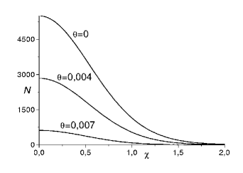
Figure 2: Mean number of photons after $n=500$ pulses (with $|g|=0.01$) versus the maximal amplitude of random phase fluctuations $\chi$ for fixed values of systematic phase deviations $\theta$.

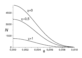
Figure 3: Mean number of photons after $n=500$ pulses (with $|g|=0.01$) versus the systematic phase deviations $\theta$, for fixed values of the amplitude of phase fluctuations $\chi$.

Fig. 2 shows the mean number of photons in the cavity after a fixed number of $n=500$ pulses (which generate approximately $\sinh^{2}(5)\approx 5500$ photons for $g=0.01$ in the case of strict resonance) versus the maximal amplitude of random phase fluctuations $\chi$ for fixed values of systematic phase deviations $\theta$. The averaging was performed in all cases over $700$ realizations consisting of $500$ random numbers $\chi_{k}$. The average values $\langle\chi_{k}\rangle=n^{-1}\sum_{k=1}^{n}\chi_{k}$ varied from $10^{-7}$ to $10^{-5}$ for each realization (so that no systematic shift was added due to random choice of $\chi_{k}$). Fig. 3 gives the mean number of photons versus $\theta$ for different fixed values of $\chi$. Fig. 4 shows the relative (and in the insertion – absolute) mean-squared deviations from the average numbers, as functions of $\chi$ for $\theta=0$. In Fig. 5, the upper curve shows the dependence of the critical amplitude of random phase fluctuations (defined by the condition that the average number of created photons after $n=500$ pulses is between $9$ and $10$) on the regular phase shift $\theta$; the lower curve gives the maximal amplitude of phase “jumps”, when the photon generation stops according to Eq. (51). It is clearly seen, that even very high level of random phase fluctuations does not stop the generation of photons, contrary to systematic phase shifts. Moreover, the critical amplitude of truely random fluctuations remains nonzero even for systematic phase shifts exceeding the value $|g|$.

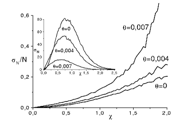
Figure 4: The relative mean-squared deviation of the number of created photons versus the maximal amplitude of random phase fluctuations $\chi$ for fixed values of systematic phase deviations $\theta$ (for $n=500$ pulses). The absolute mean-squared deviations are shown in the insertion.

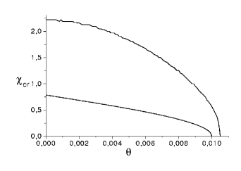
Figure 5: The dependence of the critical amplitude of random phase fluctuations on the systematic phase shift $\theta$ (the upper curve), compared with the maximal amplitude of “phase jumps”, when the photon generation stops according to Eq. (51) (the lower curve).

4.3 Analogy with resistance of disordered chains

It is worth noting that the problem of transmission through a sequence of one-dimensional barriers with randomly varying parameters (in particular, interbarrier distances) has been extensively studied in the context of solid state physics [50]. There, one of objectives is the resistance ${\cal R}$ of some chain of scatteres, expressed (in dimensionless units) by exactly the same formula (5) which gives the mean photon number in our case. In particular, Landauer [58] used a consequence of Eq. (29),

$$\frac{|\rho_{n}|^{2}}{1\!-\!|\rho_{n}|^{2}}=\frac{|\rho_{n\!-\!1}|^{2}+|r_{n}|^{2}+2|r_{n}\rho_{n\!-\!1}|\cos(\Psi_{n})}{\left(1\!-\!|\rho_{n\!-\!1}|^{2}\right)\left(1\!-\!|r_{n}|^{2}\right)},$$ (53)

$$\Psi_{n}=\zeta_{n}+2\theta_{n-1}+2\arg(s_{n-1})-\arg(\rho_{n-1}),$$

and, supposing that the phase shift $\Psi_{n}$ is a random variable, uniformly distributed over a large interval, performed averaging over $\Psi_{n}$ directly in Eq. (53), having replaced the term with $\cos(\Psi_{n})$ by zero. One can easily verify that the change of variables, $|\rho_{n}|^{2}=\tanh(y_{n})$, $|r_{n}|^{2}=\tanh(z_{n})$, transformes the set of recurrence relations (53) with $\cos(\Psi_{n})$ replaced by zero, to the equations $y_{n}=y_{n-1}+z_{n}$, whose obvious solution is $y_{n}=\sum_{k=1}^{n}z_{k}$. Thus we arrive at the following formula for the resistance of a chain with completely random distances between scatterers, uniformly distributed over sufficiently large intervals:

$${\cal R}_{n}\equiv{\cal N}_{n}=\frac{1}{2}\prod_{k=1}^{n}\frac{1+|r_{k}|^{2}}{1-|r_{k}|^{2}}-\frac{1}{2}.$$ (54)

Here $|r_{k}|^{2}$ is the energy reflection coefficient from the $k$th obstacle (barrier) and $n$ is the number of obstacles. If $|r_{n}|^{2}=|r|^{2}=const$, then (54) goes to the Landauer formula [58]

$${\cal R}_{n}\equiv{\cal N}_{n}=\frac{1}{2}\left(\frac{1+|r|^{2}}{1-|r|^{2}}\right)^{n}-\frac{1}{2}.$$ (55)

It is worth comparing Eq. (55) with Eq. (3), paying attention to different powers of the reflection coefficient $|r|$. For $n|r|^{2}>1$ formula (55) yields

$${\cal N}_{n}^{(rand)}\approx\frac{1}{2}\exp(2n|r|^{2}).$$ (56)

Consequently, totally random phase fluctuations without systematic phase shift must also lead to an exponential growth of the photon number (chain resistance), although with much more slow rate than in the resonance case, if $|r|\ll 1$. For example, for $|r|=0.01$ one needs about 500 pulses to create 5000 photons under the resonance conditions, according to Eq. (42), whereas Eq. (56) suggests that the same number of photons can appear after about $5\cdot 10^{4}$ pulses in the case of completely random fluctuations (with zero systematic phase shift).

However, removing the term proportional to $\cos(\Psi_{n})$ from the right-hand side of Eq. (53) is not well justified operation, because averaging over fluctuations of phase $\Psi_{n}$ must be performed in the final expression for ${\cal N}_{n}$, and not at some intermediate steps (as soon as $\langle f(x)\rangle\neq f(\langle x\rangle)$). Moreover, if the random variable $\Psi_{n}$ is uniformly distributed over some interval $(-\chi,\chi)$, then the average value $\langle\cos(\Psi_{n})\rangle=\sin(\chi)/\chi$ is equal (or close) to zero either if the ratio $\chi/\pi$ is an integer or if $\chi\gg 1$. In Fig. 6 we show the results of numerical calculations of the dependence of the natural logarithm $\ln\langle{\cal N}_{n}\rangle$ of the average number of photons created after $n$ pulses with completely random phase $\chi_{k}$ (defined by Eq. (50)), uniformly distributed over some large interval $(-\chi,\chi)$, for $\chi>1$ and $\theta=0$ (i.e., in the absence of systematic shifts). For each choice of $\chi$, averaging was performed over $20$ realizations.

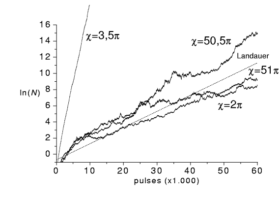
Figure 6: The natural logarithm $\mbox{ln}\langle{\cal N}_{n}\rangle$ of the average number of photons created after $n$ pulses with completely random phase $\chi_{k}$, uniformly distributed in the interval $(-\chi,\chi)$, for $\theta=0$, $g=0.01$ and different values of $\chi$. The straight line with label “Landauer” corresponds to the Landauer’s dependence (56) with $|r|=g$.

Qualitatively, we see an agreement with Landauer’s predictions: the growth of the number of photons (or equivalent resistance) is close to exponential, although the necessary number of pulses is much greater than in the case of $\chi<1$ illustrated in the Figs. 2-5. However, the results of numerical experiments are close to the asymptotical Landauer’s dependence (56), $\ln{\cal N}_{n}=2n|r|^{2}-\ln 2$ (given by the dashed straight line labeled as “Landauer”), only for integral ratios $m=\chi/\pi$ (take into account the logarithmic scale), whereas the inclinations of curves corresponding to half-integral values of the ratio $\chi/\pi=m+1/2$ (when $|\langle\cos(\chi_{n})\rangle|=[\pi(m+1/2)]^{-1}$) are much bigger for small and moderate values of $m$, approximating Landauer’s limit only when $m>100$.

The results of this section are in qualitative agreement with other studies, e.g., [31] (where quasiperiodic motions of the boundaries were considered), [55] (parametric resonance in periodic paraxial optical systems), or [53, 59, 60] (devoted to quantum oscillators with fluctuating frequencies). A possibility of generating coherent phonons in solids with time-dependent lattice strains was studied in [61]. Mathematically, this problem is reduced to quantum oscillator with time-dependent (fluctuating) frequency. Another mechanism of producing coherent phonons by femtosecond laser pulses, which is mathematically equivalent to the problem of quantum oscillator with time-dependent force, was considered recently in [62].

5 Conclusion

We have considered a simple model of photon generation from vacuum due to nonstationary (dynamical) Casimir effect in a cavity with nonequidistant spectrum of eigenfrequencies, which is reduced to the problem of quantum harmonic oscillator with time-dependent frequency. We have shown that periodic displacements of the (effective) boundary must result in exponential growth of the mean number of quanta (photons) in the selected mode under certain resonance conditions. The oscillations of the boundary need not to be monochromatic, but they must be close to periodic. However, although the period of motion of the boundary, $T_{b}$, should be adjusted to the period of field oscillations, $T_{f}$, and to some phase, depending on the concrete form of pulse, $T_{b}$ may be much greater than $T_{f}$. This result seems to be very important from the point of view of facilitating performing experiments. The concrete form of the trajectory of the wall enters the final result only through effective reflection and transmission coefficients from some “barriers” in the time dependence of the eigenfrequency.

We have studied the influence of deviations from the strict resonance, caused by systematic and random perturbations of the optimal resonance trajectory of the boundary. It appears that amplitude perturbations are less important than the phase ones. In turn, among the phase perturbations, the most dangerous for preserving the regime of photon generation are systematic deviations, which should not exceed rather low level of the order of the frequency modulation depth. On the contrary, random phase fluctuations can have much greater amplitude (even of the order of unity for zero systematic deviations) without qualitative changes in the behaviour of the system. This circumstance also seems to be important for planning future experiments, showing that some requirements might be not so rigid as one could suppose, thus diminishing the number of technical problems to be solved.

The results obtained can be easily generalized to the case when the initial state of the field mode was not vacuum, but a thermal state. Actually, one should simply multiply the right-hand side of Eq. (5) by the factor $1+2\langle n_{th}\rangle$, where $\langle n_{th}\rangle$ is the mean number of thermal photons in the initial state [8, 23, 24, 27].

However, the presented study should be considered only as a qualitative model, because many important things have not been taken into account. For example, we considered the excitation of a single selected mode, neglecting its possible interactions with other modes. Such an approach seems to be justified for cavities with nonequidistant spectra, when the boundary performs harmonic oscillations at the resonance frequency [13]. But the spectrum of anharmonic oscillations contains many frequencies. On the one hand, this fact, perhaps, explains why photons can be generated even if the period of displacements of the boundary is greater than the period of the field oscillations. On the other hand, in the presence of many frequencies some other modes can be excited, too. This question needs a detailed investigation. Also, the effects of polarization of true electromagnetic field (not its scalar model) could be important, as was shown in other examples [29, 63]. And, of course, the problem of consistent account of losses in cavities with moving nonideal mirrors must be solved (perhaps, following the lines generalizing the approaches of Refs. [18, 28, 64]).

References

- [1] G.A. Askar’yan, Zhurn. Eksp. Teor. Fiz. 42 (1962) 1672 [Sov. Phys. – JETP 15 (1962) 1161].
- [2] L.A. Rivlin, Kvant. Elektron. 6 (1979) 2248 [Sov. J. Quant. Electron. 9 (1979) 1320].
- [3] S. Sarkar, in Photons and Quantum Fluctuations, eds. E.R. Pike and H. Walther, p. 151, Hilger, Bristol, 1988.
- [4] V.V. Dodonov, A.B. Klimov, V.I. Man’ko, Phys. Lett. A 149 (1990) 225.
- [5] J. Schwinger, Proc. Nat. Acad. Sci. USA 90 (1993) 958.
- [6] E. Sassaroli, Y.N. Srivastava, A. Widom, Phys. Rev. A 50 (1994) 1027.
- [7] V.V. Dodonov, A.B. Klimov, Phys. Lett. A 167 (1992) 309.
- [8] V.V. Dodonov, A.B. Klimov, D.E. Nikonov, J. Math. Phys. 34 (1993) 2742.
- [9] G. Barton, C. Eberlein, Ann. Phys. (NY) 227 (1993) 222.
- [10] J. Cooper, IEEE Trans. Antennas Prop. 41 (1993) 1365.
- [11] C.K. Law, Phys. Rev. Lett. 73 (1994) 1931; Phys. Rev. A 49 (1994) 433; 51 (1995) 2537.
- [12] J. Dittrich, P. Duclos, P. Šeba, Phys. Rev. E 49 (1994) 3535; J. Dittrich, P. Duclos, N. Gonzalez, Rev. Math. Phys. 10 (1998) 925.
- [13] V.V. Dodonov, Phys. Lett. A 207 (1995) 126; V.V. Dodonov, A.B. Klimov, Phys. Rev. A 53 (1996) 2664.
- [14] C.K. Cole, W.C. Schieve, Phys. Rev. A 52 (1995) 4405; 64 (2001) 023813.
- [15] O. Méplan, C. Gignoux, Phys. Rev. Lett. 76 (1996) 408.
- [16] A. Lambrecht, M.-T. Jaekel, S. Reynaud, Phys. Rev. Lett. 77 (1996) 615; Eur. Phys. J. D 3 (1998) 95.
- [17] D.F. Mundarain, P.A. Maia Neto, Phys. Rev. A 57 (1998) 1379.
- [18] V.V. Dodonov, Phys. Lett. A 244 (1998) 517; Phys. Rev. A 58 (1998) 4147.
- [19] V.V. Dodonov, J. Phys. A 31 (1998) 9835.
- [20] R. Schützhold, G. Plunien, G. Soff, Phys. Rev. A 57 (1998) 2311.
- [21] D.A.R. Dalvit, F.D. Mazzitelli, Phys. Rev. A 57 (1998) 2113; 59 (1999) 3049.
- [22] R. de la Llave, N.P. Petrov, Phys. Rev. E 59 (1999) 6637.
- [23] H. Jing, Q.-Y. Shi, J.-S. Wu, Phys. Lett. A 268 (2000) 174.
- [24] M.A. Andreata, V.V. Dodonov, J. Phys. A 33 (2000) 3209.
- [25] M. Crocce, D.A.R. Dalvit, F.D. Mazzitelli, Phys. Rev. A 64 (2001) 013808.
- [26] A.V. Dodonov, V.V. Dodonov, Phys. Lett. A 289 (2001) 291; M.A. Andreata, A.V. Dodonov, V.V. Dodonov, J. Russ. Laser Res. 23 (2002) 531.
- [27] R. Schützhold, G. Plunien, G. Soff, Phys. Rev. A 65 (2002) 043820.
- [28] G. Schaller, R. Schützhold, G. Plunien, G. Soff, Phys. Rev. A 66 (2002) 023812.
- [29] M. Crocce, D.A.R. Dalvit, F.D. Mazzitelli, Phys. Rev. A 66 (2002) 033811.
- [30] J. Dittrich, P. Duclos, J. Phys. A 35 (2002) 8213.
- [31] N.P. Petrov, R. de la Llave, J.A. Vano, Physica D 180 (2003) 140.
- [32] V.V. Dodonov, in: Modern Nonlinear Optics (Adv. Chem. Phys. Series, v. 119), ed. M.W. Evans, Wiley, New York, 2001, Part 1, p.309.
- [33] G. Carugno et al, MIR project, unpublished (2002).
- [34] E. Yablonovitch, Phys. Rev. Lett. 62 (1989) 1742; S. Sarkar, Quant. Opt. 4 (1992) 345.
- [35] Y.E. Lozovik, V.G. Tsvetus, E.A. Vinogradov, Pis’ma Zh. Eksp. Teor. Fiz. 61 (1995) 711 [JETP Lett. 61 (1995) 723]; Phys. Scr. 52 (1995) 184.
- [36] V.V. Kulagin, V.A. Cherepenin, Pis’ma ZhETF 63 (1996) 160 [JETP Lett. 63 (1996) 170].
- [37] M.A. Cirone, K. Rza̧źewski, Phys. Rev. A 60 (1999) 886.
- [38] K. Husimi, Progr. Theor. Phys. 9 (1953) 381.
- [39] V.V. Dodonov, V.I. Man’ko, in: Invariants and the Evolution of Nonstationary Quantum Systems (Proc. Lebedev Physics Institute, v. 183), ed. M.A. Markov, Nova Science, Commack, 1989, p. 103.
- [40] V.V. Dodonov, in: Theory of Non-classical States of Light, eds. V.V. Dodonov and V.I. Man’ko, Taylor & Francis, London, 2003, p. 153.
- [41] V.V. Dodonov, A.B. Klimov, D.E. Nikonov, Phys. Rev. A 47 (1993) 4422.
- [42] M. Visser, Phys. Rev. A 59 (1999) 427.
- [43] L.D. Faddeev, Doklady AN SSSR 121 (1958) 63 [Sov. Phys. – Doklady 3 (1958) 747].
- [44] G.L. Lamb, Jr., Elements of Soliton Theory, Wiley, New York, 1980.
- [45] L.M. Brekhovskikh, Waves in Layered Media, Academic Press, New York, 1960.
- [46] S.Y. Karpov, S.N. Stolyarov, Usp. Fiz. Nauk 163 (1993) 63 [Physics–Uspekhi 36 (1993) 1].
- [47] W. Weinstein, J. Opt. Soc. Am. 37 (1947) 576.
- [48] M. Born, E. Wolf, Principles of Optics, Fifth edition, Cambridge University Press, Cambridge, 1975, sec. 1.6.5.
- [49] P. Yeh, A. Yariv, C.-S. Hong, J. Opt. Soc. Am. 67 (1977) 423.
- [50] P. Erdös, R.C. Herndon, Adv. Phys. 31 (1982) 65.
- [51] V.V. Dodonov, O.V. Man’ko, V.I. Man’ko, Phys. Lett. A 175 (1993) 1.
- [52] U. Bandelow, U. Leonhardt, Opt. Commun. 101 (1993) 92.
- [53] L. Ferrari, Phys. Rev. A 57 (1998) 2347; C.D.E. Boschi, L. Ferrari, Phys. Rev. A 59 (1999) 3270.
- [54] D.J. Griffiths, C.A. Steinke, Am. J. Phys. 69 (2001) 137.
- [55] S. Longhi, Opt. Commun. 176 (2000) 327.
- [56] A. Georgieva, Y.S. Kim, Phys. Rev. E 64 (2001) 026602.
- [57] J.J. Monzón, T. Yonte, L.L. Sánchez-Soto, J.F. Cariñena, J. Opt. Soc. Am. A 19 (2002) 985.
- [58] R. Landauer, Phil. Mag. 21 (1970) 863.
- [59] B. Crosignani, P. Di Porto, S. Solimeno, Phys. Rev. 186 (1969) 1342.
- [60] B.R. Mollow, Phys. Rev. A 2 (1970) 1477.
- [61] L. Ferrari, Phys. Rev. B 56 (1997) 593.
- [62] Y.E. Lozovik, V.A. Sharapov, Fiz. Tverd. Tela 45 (2003) 923 [Phys. Solid State 45 (2003) 969].
- [63] P.A. Maia Neto, L.A.S. Machado, Phys. Rev. A 54 (1996) 3420.
- [64] H. Saito, H. Hyuga, Phys. Rev. A 65 (2002) 053804.