Concurrence Vectors for Entanglement of High-dimensional Systems

Abstract

The concurrence vectors are proposed by employing the fundamental representation of $A_{n}$ Lie algebra, which provides a clear criterion to evaluate the entanglement of bipartite system of arbitrary dimension for both pure and mixed states. Accordingly, a state is separable if the norm of its concurrence vector vanishes. The state vectors related to SU(3) states and SO(3) states are discussed in detail. The sign situation of nonzero components of concurrence vectors of entangled bases presents a simple criterion to judge whether the whole Hilbert subspace spanned by those bases is entangled, or there exists entanglement edge. This is illustrated in terms of the concurrence surfaces of several concrete examples.

I Introduction

Entanglement, as one of the most intriguing features of quantum system, has been a subject of much study in recent years. It is regarded as a valuable resource in quantum computation and communication processions, which allows quantum physics to perform tasks that are classically impossible someReviews . The qubit used to be considered as the building blocks of quantum computers, and the entanglement of bipartite systems of qubits has been well studied. Most recently, moreover, an arbitrary polarization state of a single-mode biphoton was considered Zhukov to generate qutrit which is a system whose states constitute a three-dimensional Hilbert space. Experimentally, a new technique has been introduced to generate and control entangled qutritsThew , which reveals a source capable of generating maximally entangled states with a net state fidelity. The qutrit system was also suggested to be realized by nuclear magnetic resonance (NMR) utilizing deuterium nuclei partially oriented in liquid crystalline phase Kumar or by trapped ions Klimov . The use of qutrits instead of qubits was shown Bruss to be more secure against symmetric attacks on a quantum key distribution protocol while the violation of local realism for two maximally entangled $N$-dimensional state is stronger than for qubitsKaszlikowski . Thus an effective measurement of entanglement for high dimensional Hilbert space become useful.

As is known that Peres Peres96 proposed the partial transposition criterion as a necessary condition for separability (independent of the dimension of the state), which was later shown to be sufficient for the 2 by 2 and 2 by 3 cases by Horodecki et. al. MHorodecki96 . More authors carried out further discussions and proposed various proceduresRungta01 ; Badziag02 for the similar purpose. Since the concurrence introduced early by Hill and Wootters HillWootters is an important evaluation of entanglement for qubits, an systematical extension for qutrits as well as to high-dimensional system should be helpful.

In this paper we present an extension of Hill-Wootters’ concurrence on the basis of roots of $A_{n}$ Lie algebra. In next section, we define a concurrence vector whose norm can be used to evaluate the entanglement of pure states, i.e., a separable state has a vanishing norm. Its relation to other entanglement measurement is also discussed. In section III, we extend the concurrence vector to mixed states. In section IV, we discuss the concurrence surface for several concrete cases, which is expected to be helpful for the study of entanglement evolution. The advantage of our proposal is that one can easily judge whether a Hilbert subspace spanned by some entangled states is fully entangled, or there exists entanglement edge in the subspace. In the last section, a brief summary and acknowledgement are given.

II Concurrence vector for pure states: from qubits to qudits

II.1 Formal extension

Let us recall the “concurrence” introduced by Hill and Wootters

$$C(\psi)=|\langle\psi\mid\tilde{\psi}\rangle|$$

$$\mid\tilde{\psi}\rangle=(\sigma_{y}\otimes\sigma_{y})\mid\psi^{*}\rangle,$$ (1)

which provides an easy evaluation of entanglement for a pair of qubits. The qubit is a category of two-dimensional Hilbert space well described by Pauli matrices that carry out the fundamental representation of group SU(2). It is convenient to choose the SU(2) generators as $J_{z}$, $J_{+}$ and $J_{-}$ satisfying

$$[J_{z},\,J_{\pm}]=\pm J_{\pm},\;\;[J_{+},\,J_{-}]=2J_{z}.$$ (2)

In terms of these operators, Hill-Wootters’ definition (1) can be equivalently replaced by $\mid\tilde{\psi}\rangle=(J_{+}-J_{-})\otimes(J_{+}-J_{-})\mid\psi^{*}\rangle$. This expression can be conveniently extended to the case of high-dimensional Hilbert space because $\{J_{x},\,J_{y}\,J_{z}\}$ do not has counterpart for high rank groups but $\{J_{+},\,J_{-}\,J_{z}\}$ has. We need to describe a qutrit by the generators of SU(3) group. Furthermore, the SU(N) group is required for the case of $N$-dimensional Hilbert space. Hereafter, we will adopt the standard terminology in group theory in order to avoid possible ambiguities, meanwhile keeping physics picture as much as possible. Some helpful mathematical concepts are given in the appendix.

Let us analyzes the separability of the bipartite state $\mid\!\psi\rangle$. Supposing it is separable, we will have $\mid\!\psi\rangle=\mid\!\phi_{A}\rangle\otimes\mid\!\phi_{B}\rangle$ and generally $\mid\!\phi_{A}\rangle=\sum_{m=1}^{N}a_{m}\mid\!m\rangle$; $\mid\!\phi_{B}\rangle=\sum_{m=1}^{N}b_{m}\mid\!m\rangle$. The action of $E_{\alpha}$ on the state $\mid\!\phi_{A}\rangle$ (similar to $\mid\!\phi_{B}\rangle$ ) makes one term in the summation not vanish merely. This is because $E_{\alpha}$ maps some one state saying $\mid\!m^{\prime}\rangle$ to another one saying $\mid\!m^{\prime\prime}\rangle$ but the others to null. As a result, we have $\langle\phi_{1}\mid E_{\alpha}\mid\!\phi^{*}_{A}\rangle=a^{*}_{m^{\prime\prime}}a^{*}_{m^{\prime}}$. Employing the operator related to the corresponding negative root, we have $\langle\phi_{1}\mid E_{-\alpha}\mid\!\phi^{*}_{A}\rangle=a^{*}_{m^{\prime}}a^{*}_{m^{\prime\prime}}$. Referring to Hill and Wootters strategy for two-qubit case, one can extend the concept of concurrence to a concurrence vector defined by

$${\bf C}=\{\langle\psi\mid(E_{\alpha}-E_{-\alpha})\otimes(E_{\beta}-E_{-\beta})\mid\!\psi^{*}\rangle\mid\alpha,\beta\in\Delta^{+}\},\\$$ (3)

where $\Delta^{+}$ denotes the set of positive roots of $A_{N-1}$ Lie algebra. As there are totaly $N(N-1)/2$ positive roots, the concurrence vector is a $N^{2}(N-1)^{2}/4$ dimensional vector. The criterion for the separability of a joint pure state of bipartite system of arbitrary dimension is that the norm of the concurrence vector is zero, otherwise the state is entangled.

II.2 The relation to other entanglement measurements

In above we proposed concurrence vector on the basis of mathematics analogy. It is worthwhile to observe the relationship between the afore introduced concurrence vector and other entanglement measurement.

For a pair of qubit and qutrit which can be regarded as a pair of spin-$1/2$ and spin-1, the concurrence vector is a three dimensional vector given by

$$\textbf{C}=\{\langle\psi\,\mid(\sigma_{+}-\sigma_{-})\otimes(E_{\alpha}-E_{-\alpha})\mid\!\psi^{*}\rangle\,\mid\alpha\in\Delta^{+}\}$$ (4)

where $\sigma_{\pm}=(\sigma_{x}\pm i\sigma_{y})/2$, and $\Delta^{+}$ for $A_{2}$ contains three positive roots. Thus the concurrence vector here is of three dimension. As we known, any state of bipartite system can be expanded as

$$|\psi\rangle=\sum_{\mu,j}a_{\mu j}|\mu\rangle\otimes|j\rangle,$$ (5)

where $a_{\mu j}$ is complex coefficients, and in our present case, $\mu=1,2$ and $j=1,2,3$. It is easy to obtain the norm of concurrence, $|\mathbf{C}|^{2}=C^{2}_{1}+C^{2}_{2}+C^{2}_{3}=4(a_{11}a_{22}-a_{12}a_{21})^{2}+4(a_{12}a_{23}-a_{13}a_{22})^{2}+4(a_{11}a_{23}-a_{13}a_{21})^{2}$.

In order to show the reliability of concurrence vector, we consider the von Neumann entropy. The reduced density matrix $\rho_{A}$ and $\rho_{B}$ can be easily obtained,

$$\rho_{A}=aa^{\dagger}=\left(\begin{array}[]{ccc}a_{11}&a_{12}&a_{13}\\ a_{21}&a_{22}&a_{23}\\ \end{array}\right)\left(\begin{array}[]{cc}a_{11}^{\ast}&a_{21}^{\ast}\\ a_{12}^{\ast}&a_{22}^{\ast}\\ a_{13}^{\ast}&a_{23}^{\ast}\\ \end{array}\right).$$

It is a $2\times 2$ matrix, thus there are two eigenvalues $\kappa_{1}^{2}$ and $\kappa_{2}^{2}$, that are squares of the coefficients of Schmidt decomposition $|\psi\rangle=\kappa_{1}|x_{1}\rangle_{A}|y_{1}\rangle_{B}+\kappa_{2}|x_{2}\rangle_{A}|y_{2}\rangle_{B}$. Here the $\kappa_{1}^{2}$ and $\kappa_{2}^{2}$ are the roots of the following secular equation

$$\lambda^{2}-\lambda+|\mathbf{C}|^{2}/4=0,$$ (7)

where $|\mathbf{C}|$ is precisely the norm of concurrence vector we proposed.

From Eq.(7), we obtain

$$\kappa_{1,2}^{2}=\frac{1\pm\sqrt{1-|\mathbf{C}|^{2}}}{2}.$$ (8)

So the von Neumann entropy is given by

$$E_{N}(|\psi\rangle)=h((1-\sqrt{1-|\mathbf{C}|^{2}})/2),$$ (9)

where

$$h(x)=-x\log_{2}x-(1-x)\log_{2}(1-x).$$

On the other hand, one obtain $\rho_{B}$ by tracing out the degree of freedom of part A, i.e.,

$$\rho_{B}=a^{\dagger}a.$$ (10)

This is a $3\times 3$ matrix whose eigenvalues are denoted by $\tilde{\kappa}_{1}^{2}$, $\tilde{\kappa}_{2}^{2}$, $\tilde{\kappa}_{3}^{2}$ are roots of the algebraic equation

$$\lambda^{3}-\lambda^{2}+\frac{|\mathbf{C}|^{2}}{4}\lambda-\det(\rho_{B})=0.$$ (11)

The reduced density matrix $\rho_{B}$ is of rank 2, i.e., $\det\rho_{B}=0$, then there are only two non-zero eigenvalues. The von Neumann entropy takes the same form as in Eq.(9). Just like the case of WoottersWootters , the von Newmann entropy here is also a monotonous function of the norm of concurrence vectors: $|{\bf C}|^{2}$. Therefore, the concurrence vector is a reliable measurement of entanglement of the states of qubit-qutrit system.

For bipartite qutrit system, the general state can be written as

$$|\psi\rangle=\sum_{i,j}g_{ij}|i\rangle\otimes|j\rangle$$ (12)

where $i$, $j=1,2,3$. The reduced density matrix $\rho_{B}={\rm tr}_{A}|\psi\rangle\langle\psi|\equiv g^{\dagger}g$, is clearly a positive-definite matrix, in which $g=\mathrm{mat}(g_{ij})$. Let $\kappa_{1}^{2}$, $\kappa_{2}^{2}$, $\kappa_{3}^{2}$ be the eigenvalues of $\rho_{B}$, which solve the following algebraic equation

$$\lambda^{3}-\lambda^{2}+\frac{|\mathbf{C}|^{2}}{4}\lambda-\det\rho_{B}=0,$$ (13)

where $|\mathbf{C}|^{2}$ is just the square of the norm of the concurrence vector we proposed, namely,

$$|\mathbf{C}|^{2}=4(\kappa_{1}^{2}\kappa_{2}^{2}+\kappa_{2}^{2}\kappa_{3}^{2}+\kappa_{3}^{2}\kappa_{1}^{2}).$$

The calculation of the von Neumann entropy exhibits an explicit relation to the norm of concurrence vector,

$$E_{N}(|\psi\rangle)=h\bigl{(}x^{+},x^{-}\bigr{)},\\$$

where

$$h(x^{+},x^{-})=-x^{+}\log x^{+}-x^{-}\log x^{-}$$

$$-(1-x^{+}-x^{-})\log(1-x^{+}-x^{-}),$$ (14)

and

$$x^{\pm} = \frac{1}{3}+e^{\pm i\frac{2\pi}{3}}\sqrt[3]{-\frac{q}{2}+\sqrt{\frac{q^{2}}{4}+\frac{p^{3}}{27}}}$$

$$+ e^{\mp i\frac{2\pi}{3}}\sqrt[3]{-\frac{q}{2}-\sqrt{\frac{q^{2}}{4}+\frac{p^{3}}{27}}},$$

$$p = \frac{|\mathbf{C}|^{2}}{4}-\frac{1}{3}$$

$$q = \det\rho_{B}+\frac{2}{27}-\frac{|\mathbf{C}|^{2}}{12}.$$

Clearly, the von Neumann entropy depends on the norm of the concurrence vector monotonically. Unlike the von Neumann entropy for qubit which depends only on the concurrence HillWootters , it also depends on the determinate of the reduced density matrix. The supremum (dash line) and infimum for the von Neumann entropy versus $|C|$ are plotted in Fig.1, where both points of the entanglement maximum and non-entanglement coincide. It is clearly a convex function.

Figure 1: The von Neumann entropy versus the norm of concurrence vector. Dash line is the supremum and solid line the infimum

The linear entropy, also a measurement of entanglement, is given by

$$E_{L}(|\psi\rangle) = 1-tr\rho_{B}^{2}$$

$$= (\kappa_{1}^{2}+\kappa_{2}^{2}+\kappa_{3}^{2})^{2}-\bigl{(}\kappa_{1}^{4}+\kappa_{2}^{4}+\kappa_{3}^{4}\bigr{)}$$

$$= 2(\kappa_{1}^{2}\kappa_{2}^{2}+\kappa_{2}^{2}\kappa_{3}^{2}+\kappa_{3}^{2}\kappa_{1}^{2})=|\mathbf{C}|^{2}/2$$

which indicates a direct relation to the norm of concurrence vector. The magnitude of the linear entropy arranges from 0 to $1-1/d$ (here $d=3$). It is clearly a monotonically increasing function versus the norm of concurrence vector. Hence the concurrence vector we proposed is a reasonable measurement of entanglement for qutrits

II.3 Qutrit via SU(3) states

Now we consider the qutrit as a concrete example. The states $\mid\!1\rangle$, $\mid\!2\rangle$ and $\mid\!3\rangle$ and the corresponding weights (denoted by black dots) $[1/2,0]$, $[-1/2,\,1/2]$ and $[0,\,-1/2]$ are plotted in the following

This represents the fundamental representation of SU(3). It is well known that the direct product representation is reduced to two irreducible representations, i.e., ${\bf 3\otimes 3=3^{*}\oplus 6}$. The bases for the ${\bf 3^{*}}$ dimensional representation are all entangled states, $\mid\!\psi^{-}_{1}\rangle$, $\mid\!\psi^{-}_{2}\rangle$, $\mid\!\psi^{-}_{3}\rangle$, but they are not the maximally entangled states. Additionally, it is not possible to produce maximally entangled state by superposition in this subspace.

Among the bases for the ${\bf 6}$ dimensional representation ( hexad), $\mid\!\psi^{+}_{1}\rangle$, $\mid\!\psi^{+}_{2}\rangle$ and $\mid\!\psi^{+}_{3}\rangle$ are entangled (not maximally entangled) states, but the other three $\mid\!11\rangle$, $\mid\!22\rangle$ and $\mid\!33\rangle$ are not entangled states. Whereas, three maximally entangled states, $\mid\!\varphi_{1}\rangle$, $\mid\!\varphi_{2}\rangle$ and $\mid\!\varphi_{3}\rangle$ can be obtained by superposition of those three states. All the mentioned states are given in the following

$$\mid\!\varphi_{1}\rangle=\frac{1}{\sqrt{3}}\bigl{(}\mid\!11\rangle+\mid\!22\rangle+\mid\!33\rangle\bigr{)},$$

$$\mid\!\varphi_{2}\rangle=\frac{1}{\sqrt{3}}\bigl{(}\mid\!11\rangle+e^{i2\pi/3}\mid\!22\rangle+e^{-i2\pi/3}\mid\!33\rangle\bigr{)},$$

$$\mid\!\varphi_{3}\rangle=\frac{1}{\sqrt{3}}\bigl{(}\mid\!11\rangle+e^{-i2\pi/3}\mid\!22\rangle+e^{i2\pi/3}\mid\!33\rangle\bigr{)},$$

$$\mid\!\psi^{\pm}_{1}\rangle=\frac{1}{\sqrt{2}}\bigl{(}\mid\!12\rangle\pm\mid\!21\rangle\bigr{)},$$

$$\mid\!\psi^{\pm}_{2}\rangle=\frac{1}{\sqrt{2}}\bigl{(}\mid\!23\rangle\pm\mid\!32\rangle\bigr{)},$$

$$\mid\!\psi^{\pm}_{3}\rangle=\frac{1}{\sqrt{2}}\bigl{(}\mid\!13\rangle\pm\mid\!31\rangle\bigr{)}.$$ (15)

The above nine states are orthonormal to each other. Their concurrence vectors are calculated to be

$$\mathbf{C}_{\mid\!\varphi_{1}\rangle} = (\frac{2}{3},\,0,\,0,\,0,\,\frac{2}{3},\,0,\,0,\,0,\,\frac{2}{3})$$

$$\mathbf{C}_{\mid\!\varphi_{2}\rangle} = (\frac{2}{3}e^{-i2\pi/3},0,0,0,\frac{2}{3},0,0,0,\frac{2}{3}e^{i2\pi/3})$$

$$\mathbf{C}_{\mid\!\varphi_{3}\rangle} = (\frac{2}{3}e^{i2\pi/3},0,0,0,\frac{2}{3},0,0,0,\frac{2}{3}e^{-i2\pi/3})$$

$$\mathbf{C}_{\mid\!\psi^{\pm}_{1}\rangle} = (\mp 1,\,0,\,0,\,0,\,0,\,0,\,0,\,0,\,0)$$

$$\mathbf{C}_{\mid\!\psi^{\pm}_{2}\rangle} = (0,\,0,\,0,\,0,\,\mp 1,\,0,\,0,\,0,\,0)$$

$$\mathbf{C}_{\mid\!\psi^{\pm}_{3}\rangle} = (0,\,0,\,0,\,0,\,0,\,0,\,0,\,0,\,\mp 1)$$ (16)

In addition to $\mid\!\varphi_{1}\rangle,\,\cdots$, $\mid\!\varphi_{3}\rangle$, there are six more orthonormal bases,

$$\mid\!\varphi_{4}\rangle=(\mid\!12\rangle+\mid\!23\rangle+\mid\!31\rangle)/\sqrt{3},$$

$$\mid\!\varphi_{5}\rangle=(\mid\!12\rangle+e^{i2\pi/3}\mid\!23\rangle+e^{-i2\pi/3}\mid\!31\rangle)/\sqrt{3},$$

$$\;\;\cdots,$$

$$\mid\!\varphi_{9}\rangle=(\mid\!21\rangle+e^{-i2\pi/3}\mid\!32\rangle+e^{i2\pi/3}\mid\!13\rangle)/\sqrt{3},$$

which were adopted as a generalization of EPR pairs when discussing teleportation Bennet93 . The concurrence vectors for those states are easily calculated, for example, $\mathbf{C}=(0,2/3,0,0,0,-2/3,-2/3,0,0)$ for $\mid\!\varphi_{4}\rangle$. Actually, all the states $\mid\!\varphi_{l}\rangle$, ($l=4,\cdots,\,9$) are shown to be maximally entangled by calculating the norm of their concurrence vectors $|{\bf C}|^{2}=4/3$.

II.4 Qutrit via SO(3) states

The fundamental representation of SU(2) is carried out by spin-1/2 system which refers to the qubit. We know the Bell bases, $\mid\!\psi^{B}_{\pm}\rangle=\bigl{(}\mid\!\uparrow\downarrow\rangle\pm\mid\!\downarrow\uparrow\rangle\bigr{)}/\sqrt{2}$, $\mid\!\varphi^{B}_{\pm}\rangle=\bigl{(}\mid\!\uparrow\uparrow\rangle\pm\mid\!\downarrow\downarrow\rangle\bigr{)}/\sqrt{2}$ are simultaneous eigenstates of $S_{x}\otimes S_{x}$ and $S_{z}\otimes S_{z}$, which is not valid for spin-1 (i.e., SO(3) representation) or high spin systems. This is because $S_{x}\otimes S_{x}$, $S_{y}\otimes S_{y}$ and $S_{z}\otimes S_{z}$ commute to each other only for spin-1/2 case. We consider such a pair of qutrits that their direct product representation decomposes into SO(3) irreducible representations, i.e., ${\bf 3\otimes 3=5\oplus 3\oplus 1}$. Some of their states read,

$$\mid\!\chi^{\pm}_{1}\rangle=\frac{1}{\sqrt{2}}\bigl{(}\mid\!01\rangle\pm\mid\!10\rangle\bigr{)},$$

$$\mid\!\chi^{\pm}_{-\!1}\rangle=\frac{1}{\sqrt{2}}\bigl{(}\mid\!-\!10\rangle\pm\mid\!0-\!\!1\rangle\bigr{)},$$

$$\mid\!\chi^{\pm}_{0}\rangle=\frac{1}{\sqrt{4\pm 2}}\bigl{(}\mid\!-\!11\rangle\pm\mid\!00\rangle+\mid\!00\rangle\pm\mid\!1-\!\!1\rangle\bigr{)},$$

$$\mid\!\chi^{0}_{0}\rangle=\frac{1}{\sqrt{3}}\bigl{(}\mid\!-\!11\rangle-\mid\!00\rangle+\mid\!1-\!\!1\rangle\bigr{)},$$

$$\mid\!\phi^{\pm}\rangle=\frac{1}{\sqrt{2}}\bigl{(}\mid\!11\rangle\pm\mid\!-\!1-\!\!1\rangle\bigr{)}.$$ (17)

It is easy to calculate their concurrence vectors:

$$\mathbf{C}_{\mid\!\chi^{\pm}_{1}\rangle} = (\mp 1,\,0,\,0,\,0,\,0,\,0,\,0,\,0,\,0)$$

$$\mathbf{C}_{\mid\!\chi^{\pm}_{-1}\rangle} = (0,\,0,\,0,\,0,\,\mp 1,\,0,\,0,\,0,\,0)$$

$$\mathbf{C}_{\mid\!\chi^{-}_{0}\rangle} = (0,\,0,\,0,\,0,\,0,\,0,\,0,\,0,\,1)$$

$$\mathbf{C}_{\mid\!\chi^{+}_{0}\rangle} = (0,-\frac{2}{3},0,-\frac{2}{3},0,0,0,0,-\frac{1}{3})$$

$$\mathbf{C}_{\mid\!\chi^{0}_{0}\rangle} = (0,\frac{2}{3},0,\frac{2}{3},0,0,0,0,-\frac{2}{3})$$

$$\mathbf{C}_{\mid\!\phi^{\pm}\rangle} = (0,\,0,\,0,\,0,\,0,\,0,\,0,\,0,\pm 1)$$ (18)

The evaluation of the norm of concurrence vector indicates that the singlet $\mid\!\chi^{0}_{0}\rangle$ is maximally entangled $|{\bf C}|^{2}=4/3$; the triplet, $\mid\!\chi^{-}_{j}\rangle$ (hereafter for SO(3) $j=-1,0,1$) are entangled but not maximally entangled $|{\bf C}|^{2}=1$; among the pentads only $\mid\!\chi^{+}_{j}\rangle$ are entangled states while $\mid\!11\rangle$ and $\mid\!-1-1\rangle$ are unentangled states whose superposition provides the two entangled states, $\mid\!\phi^{\pm}\rangle$.

III Concurrence vector for mixed states

In the light of our extension of the measurement of entanglement in terms of concurrence vector for pure states, it is natural to introduce

$$\mid\!\tilde{\psi}\rangle_{\alpha\beta}=(E_{\alpha}-E_{-\alpha})\otimes(E_{\beta}-E_{-\beta})\mid\!\psi^{*}\rangle,$$ (19)

here $\alpha$ and $\beta$ refer to the aforementioned positive roots of $A_{N-1}$ Lie algebra. Similar to the strategy of WoottersWootters , we define some matrices given by

$$\tau^{\alpha\beta}_{ij}=\langle v_{i}\,\mid(E_{\alpha}-E_{-\alpha})\otimes(E_{\beta}-E_{-\beta})\mid\!v_{j}^{*}\rangle$$ (20)

where $\{\mid\!v_{i}\rangle\mid i=1,\,2,\cdots\}$ are the eigenvectors of the density matrix $\rho$ which characterizes a given mixed state. Apparently, the matrices $(\tau_{ij})$ are symmetric. According to Takagi’s factorization horn , for any symmetric matrix $A$, there exists a unitary $U$ and a real nonnegative diagonal matrix $d=\mathrm{diag}(\lambda_{1},\ldots,\lambda_{n})$ such that $A=Ud~{}U^{T}$ and the diagonal entries of $d$ are the nonnegative square roots of the corresponding eigenvalues of $AA^{\ast}$. Thus there exists a decomposition $\mid\!x_{i}\rangle=U_{ij}^{*}\mid\!v_{j}\rangle$ satisfying

$$\langle x_{i}\,\mid(E_{\alpha}-E_{-\alpha})\otimes(E_{\beta}-E_{-\beta})\mid\!x^{*}_{j}\rangle$$

$$=(U\tau^{\alpha\beta}U^{T})_{ij}=\lambda_{i}^{\alpha\beta}\delta_{ij}.$$ (21)

Here $\lambda^{\alpha\beta}_{i}$ is the nonnegative square root of the eigenvalue of $\tau^{\alpha\beta}\tau^{\ast\alpha\beta}$ and

$$\tau^{\alpha\beta}\tau^{\alpha\beta\ast}=\sqrt{\rho}(E_{\alpha}-E_{-\alpha})\otimes\hskip 28.45274pt$$

$$(E_{\beta}-E_{-\beta})\rho^{\ast}(E_{\alpha}-E_{-\alpha})\otimes(E_{\beta}-E_{-\beta})\sqrt{\rho}.$$ (22)

One can make another decomposition of $\rho$ in terms of $\{\mid\!y_{i}\rangle\}$,

$$|y_{1}\rangle=|x_{1}\rangle;\ \ |y_{j}\rangle=i|x_{j}\rangle,\quad j\neq 1$$ (23)

If one repeat the steps given by Wootters in Ref.Wootters , one can show that for some given positive roots $\alpha$, $\beta$, the concurrence is expressed as

$$C^{\alpha\beta}=\max\{0,\,\lambda_{1}^{\alpha\beta}-\sum_{i=2}^{n}\lambda_{i}^{\alpha\beta}\}$$

where $\lambda^{\alpha\beta}_{1}=\max\{\lambda^{\alpha\beta}_{i},i=1,\ldots,N\}$. Thus we derive a formula to calculate concurrence vector for mixed state. Then the norm of such a concurrence vector can be employed to measure the entanglement of mixed state:

$$|\mathbf{C}|^{2}=\sum_{\alpha\beta}|C_{\alpha\beta}|^{2}$$ (24)

For SU(2) case there is only one positive root, which corresponds to a pair of qubits, the concurrence vector (24) is one dimensional, which is just the original definition of Wootters’ concurrence. The concurrence vector in Eq. (24) is expected to study the pairwise entanglement of SU(3) Heisenberg model similar to the strategy of XXZ chain Gu03 which is in progress.

IV Concurrence surface and entanglement edge

Calculating the norm of the concurrence vectors for an arbitrary normalized state in the three-dimensional subspace spanned by either $\{\mid\!\psi^{-}_{1}\rangle,\,\mid\!\psi^{-}_{2}\rangle,\,\mid\!\psi^{-}_{3}\rangle\}$, or $\{\mid\!\psi^{+}_{1}\rangle,\,\mid\!\psi^{+}_{2}\rangle,\,\mid\!\psi^{+}_{3}\rangle\}$, or $\{\mid\!\varphi_{1}\rangle,\,\mid\!\varphi_{2}\rangle,\,\mid\!\varphi_{3}\rangle\}$ respectively, we obtain several conclusions. Any states in the space of the former two cases yield a constant norm of concurrence vectors, which means that the Hilbert subspace manifests a fixed entanglement. The norm of concurrence vector vanishes in the third case when the expanding coefficients take some particular magnitudes. This indicates that some states in that Hilbert subspace are separable. Braunstein et al. Braunstein99 analyzed the separability of $N$-qubit states near the maximally mixed state. Vidal and Tarrach Vidal99 give a separability boundary for the mixture of the maximally mixed state with a pure state. Caves and Milburn Caves00 discussed the lower and upper bounds on the size of the neighborhood of separable states around the maximally mixed state of qutrits. One will see in the following that all these become easily understandable by making use of the concept of concurrence vectors.

The entanglement features of those three Hilbert subspaces discussed previously arise from the sign properties of the concurrence vectors. Considering a Hilbert subspace constituted by some bases obeying

$$\langle\psi_{\mu}\mid\tilde{\psi_{\nu}}\rangle_{\alpha\beta}\propto\delta_{\mu\nu}$$ (25)

where $\mid\!\tilde{\psi_{\nu}}\rangle_{\alpha\beta}$ is defined by Eq.(19). One immediate criterion is that the state vectors lie in the Hilbert subspace are all entangled as long as the corresponding nonzero components of the concurrence vectors for those bases have the same signs (i.e., positive or negative), which implies impossible to make a superposition state with all the components of the concurrence vector vanish.

It is instructive to observe the entanglement edges in the subspace of the $6$ dimensional representation of SU(3). Since the norm of concurrence vectors are constant in the subspace spanned by $\mid\!\psi^{+}_{j}\rangle$, we let the coefficients of these three bases equal to $p$. We also choose the coefficients for $\mid\!11\rangle$, $\mid\!22\rangle$ and $\mid\!33\rangle$ to be the same $q$ so that to plot a three dimensional picture. The curve of the norm of concurrence vector versus $p$ and $q$ is given in Fig.(2), the left. When $p\rightarrow\sqrt{2}q$ and $q\rightarrow 1/\sqrt{3}$ it approaches the entanglement edge.

Now we consider the case for SO(3). As nonzero components of concurrence vectors for the triplet are positive and that for the three entangled bases in the pentad are negative, both the whole Hilbert subspace spanned by $\{\mid\!\chi^{-}_{j}\rangle\}$ and the subspace spanned by $\{\mid\!\chi^{+}_{j}\rangle\}$ are entangled. Because the nonzero components of concurrence vectors for $\mid\!\phi^{+}\rangle$ is positive but that for $\mid\!\phi^{-}\rangle$ is negative (see Eq.(II.4)), the five dimensional Hilbert subspace spanned by $\{\mid\!\chi^{+}_{j}\rangle\}$ and $\mid\!\phi^{\pm}\rangle$ are not fully entangled.

The parameter space of general states in some three dimensional Hilbert subspace is described by a two-sphere $(\theta,\,\phi)$ and a phase factor $e^{i\delta}$ which is fixed to unit without loss of generality. It is illuminative to observe the geometry structures by plotting the norm of concurrence vector as radial coordinate, i.e., $r(\theta,\,\phi)=\mid{\bf C}_{\mid\!\theta,\,\phi\rangle}\mid$, we call it concurrence surface. The concurrence surfaces for the triplets of either SO(3) or SU(3) is simply a sphere of unit radius, which encloses a spheroid of volume $4\pi/3$. The concurrence surface for the Hilbert subspace spanned by the three maximally entangled states $\{\varphi_{j}\}$ of SU(3) is plotted in Fig.2 (the right), whose enclosure merely occupies $13.5\%$ more volume than a unit spheroid does though their bases are maximally entangled. This is obviously due to the presence of entanglement edges. The concurrence surfaces for the Hilbert subspace spanned by the three originally entangled states in the pentad (left figure), and that spanned by the singlet together with $\mid\!\varphi^{\pm}\rangle$ are plotted in Fig.3 (right figure). Their enclosures occupy volumes of $3.18868$ and $2.75916$ respectively, the later is smaller though one of its bases is maximally entangled.

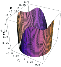
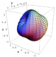
Figure 2: (Color online) The left is the relation of $\mid{\bf C}\mid$ versus $p$ and $q$ for state $p(\mid\!\psi^{+}_{1}\rangle+\mid\!\psi^{+}_{2}\rangle+\mid\!\psi^{+}_{3}\rangle)+q(\mid\!11\rangle+\mid\!22\rangle+\mid\!33\rangle)$. The right is the surface $|{\bf C}(\theta,\,\phi)|$ for Hilbert subspace $\sin\theta\cos\phi\mid\!\varphi_{1}\rangle+\sin\theta\sin\phi\mid\!\varphi_{2}\rangle+\cos\theta\mid\!\varphi_{3}\rangle)$

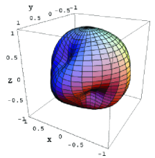
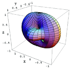
Figure 3: (Color online) The surfaces $\mid{\bf C}(\theta,\,\phi)\mid$ for the Hilbert subspaces $\sin\theta\cos\phi\mid\!\chi^{+}_{1}\rangle+\sin\theta\sin\phi\mid\!\chi^{+}_{0}\rangle+\cos\theta\mid\!\chi^{+}_{-1}\rangle$ (left), and $\sin\theta\cos\phi\mid\!\chi^{0}_{0}\rangle+\sin\theta\sin\phi\mid\!\phi^{+}\rangle+\cos\theta\mid\!\phi^{-}\rangle$ (right).

Quantum entanglement implies correlations between the results of measurements on component subsystems of a larger physical system, which can not be understood by means of correlations between local classical properties inherent in those subsystems. Wang and Zanardi WangZanardi02 studied the entanglement of unitary operators on a bipartite quantum systems that is related to the entangling power of the associated quantum evolutions. It maybe useful to associate those topics with the evolution of concurrence vectors. Zanardi and Rasetti Zandardi99 showed that the notion of generalized Berry phase can be used for enabling quantum computation, which also supports the necessity of the investigation on the parameter manifold related to quantum system with high rank symmetries.

V Summary

In above we proposed a concurrence vector to measure the entanglement of bipartite system of arbitrary dimension by employing the fundamental representation of $A_{n}$ ($n=N-1$) Lie algebra. For pure state, we have discussed the relation between the concurrence vector and the von Neumann entropy for both qubit-qutrit pair and qutrit-qutrit pair. We also gave a formula to calculate the norm of concurrence vector for mixed states on the basis of the strategy of Wootters. We have shown that the norm of concurrence vector can be used to evaluate the entanglement of a state, i.e., a separable state has a vanishing norm. However, we have not yet found an example such that the entanglement of UPB state or PPT state with no product vectors in its range can be detected by calculating concurrence vector. Another advantage of concurrence vectors is easy to judge whether a Hilbert subspace spanned by some entangled bases is fully entangled states, or there exists entanglement edge in the subspace. If the corresponding nonzero components of concurrence vectors of the basis states are all positive or all negative, all the state vectors lie in this Hilbert subspace are entangled. We calculated the concurrence vectors for the states related to SU(3) and SO(3) explicitly. We also discussed concurrence surface and compared the volumes enclosed by the surface for various cases. Their geometry will be useful for understanding the entanglement capacities in various Hilbert subspaces.

Appendix A

As the qutrit can be related by the generators of the SU(3) group and the $N$-dimensional Hilbert space by that of the SU(N) group. According to Cartan-Weyl analysis, the generators can be divided into two sets: the Cartan subalgebra which is the maximal Abelian subalgebra, and the remaining generators which play the similar role as the above $J_{\pm}$. The structure constants for the commutation relations of those operators can be described by the called root space diagram. The root space diagram for $A_{2}$ Lie algebra has a hexagonal shape,

The double circle at the center indicates the existence of two generators $H_{1}$, $H_{2}$ in the Cartan subalgebra. Unlike the spin systems whose states are labelled by the eigenvalue of $J_{z}$ which is the called magnetic quantum number, the states of SU(3) system are labelled by the eigenvalues of $(H_{1},\,H_{2})$ that is therefore a vector called weight vector. We adopt nonorthogonal bases to expend the root vectors choosing the simple roots ${\bf\alpha}_{1}$ and ${\bf\alpha}_{2}$ as coordinate bases, which is clear and convenient for physicists. Placing contravariant components, $({\bf\alpha})^{i}$ in conventional parenthesis, we have the positive roots ${\bf\alpha}_{1}=(1,\,0)$, ${\bf\alpha}_{2}=(0,\,1)$, ${\bf\alpha}_{1}+{\bf\alpha}_{2}=(1,\,1)$, and the negative roots $-{\bf\alpha}_{1}=(-1,\,0)$, $-{\bf\alpha}_{2}=(0,\,-1)$, $-{\bf\alpha}_{1}-{\bf\alpha}_{2}=(-1,\,-1)$. If placing covariant components, $({\bf\alpha})_{j}$, in square parenthesis, we easily obtain from the above root space diagram that ${\bf\alpha}_{1}=[1,\,-1/2\,]$, ${\bf\alpha}_{2}=[-1/2,\,1\,]$, ${\bf\alpha}_{1}+{\bf\alpha}_{2}=[1/2,\,1/2\,]$, $-{\bf\alpha}_{1}=[-1,\,1/2\,]$, $-{\bf\alpha}_{2}=[1/2,\,-1\,]$, and $-{\bf\alpha}_{1}-{\bf\alpha}_{2}=[-1/2,\,-1\,]$. Then one can easily write out the following commutation relations

$$\bigl{[}H_{i},\,H_{j}\bigr{]}=0,\hskip 28.45274pt$$ (26)

$$\bigl{[}H_{j},\,E_{\bf\alpha}\bigr{]}=({\bf\alpha})_{j}E_{\bf\alpha}, \bigl{[}E_{\bf\alpha},\,E_{-\bf\alpha}\bigr{]}=2({\bf\alpha})^{i}H_{i},$$

$$\bigl{[}E_{\bf\alpha},\,E_{\bf\beta}\bigr{]}=E_{\bf\alpha+\beta}\hskip 11.38109pt \;{\rm if}\;\;{\bf\alpha+\beta}\in\Delta.$$

where $\Delta$ denotes the set of nonzero roots of nonexceptional Lie algebra. The above commutation relations imply that $E_{\pm\alpha_{j}}$ play the roles of raising/lowering operators like $J_{\pm}$ of the angular momentum operator. Moreover, there are more than one operators, $H_{j}$’s, that commute to each other. For SU(N) case which corresponds to $A_{N-1}$ Lie algebra, there are $N-1$ generators in the Cartan subalgebra, hence $i,j=1,...,N-1$ and Eq.(26) also fulfil. Due to $N-1$ dimensional vectors are difficult to depict, the root space diagram is represented graphically by a two dimensional diagram, called Dynkin diagram:

where each open dot ”$\circ$” denotes a simple root, the angle between a pair of simple roots is $120^{o}$ if a line connecting them; that is $90^{o}$ if no line connecting them. Their covariant components of simple roots are easily calculated from the Dynkin diagram,

$$\alpha_{1}=[1,\,-1/2,\;\;0,\hskip 8.53581pt\cdots\hskip 17.07164pt,0],$$

$$\alpha_{2}=[-1/2,\,1,\,-1/2,\,0,\cdots,0],$$

$$\;\;\cdots,$$

$$\alpha_{N-1}=[0,\,0,\cdots,0,\,-1/2,\,1\,].$$ (27)

The simple roots are normalized to unity so that the structure constants in Eq. (26) differs from the Cartan matrix in textbook of group theory by a factor $1/2$. The advantage of our convention is that if returning to the SU(2), whose root space diagram has a simple line shape,

the eigenvalues of $S_{z}$ are $1/2$ and $-1/2$ respectively for spin up and down, otherwise, they would be $1$ and $-1$.

We consider an $N$-dimensional Hilbert space which carries out the fundamental representation of Lie algebra $A_{N-1}$, the whole weight vectors that label the state bases can be easily produced from the highest weight vector $[1/2,0,\,\cdots]$ by Weyl reflection which is easily realized by means of the covariant component of simple roots, i.e.,
$[\frac{1}{2},\,0,\,\cdots]\shortstack{ -$\alpha_{1}$ \\ $\longrightarrow$ }[0.0pt]\shortstack{$-\alpha_{2}$ \\ $\longrightarrow$}\cdots\shortstack{$-\alpha_{N-1}$\\ $\longrightarrow$}[0.0pt].$
Consequently, the $N$ state vectors are generated by the lowering operators.

$$\mid\!1\rangle\shortstack{$E_{-\alpha_{1}}$ \\ $\longrightarrow$}\mid\!2\rangle\shortstack{$E_{-\alpha_{2}}$ \\ $\longrightarrow$}\cdots\mid\!N-1\rangle\shortstack{$E_{-\alpha_{N-1}}$ \\ $\longrightarrow$}\mid\!N\rangle.$$ (28)

The positive simple roots, whereas, just give the reverse of the above relations.

References

• (1) C.H. Bennett, and D.P. Divincenzo, Nature 404, 247 (2000). M. A. Nielsen and I. L. Chuang, Quantum Computation and Quantum Communication (Cambridge University Press, Cambridge, 2000).
• (2) A.A. Zhukov, G.A. Maslennikov, M.V. Chekhova, JETP Letters 76(10), 596-599 (2002); quant-ph/0305113
• (3) R.T. Thew, A.Acin, H.Zbinden, N.Gisin, preprint, quant-ph/0307122
• (4) R. Das, A. Mitra, V. Kumar and A. Kumar, quant-ph/0307240
• (5) A.B. Klimov, R. Guzman, J.C. Retamal, and S. Saavedra, Phys.Β Rev.Β A 67, 062313 (2003).
• (6) D. Bruss and C Macchiavello, Phys.Β Rev.Β Lett. 88, 127901 (2002).
• (7) D. Kaszlikowski, P. Gnacinski, M. Zukowski et.al., Phys.Β Rev.Β Lett. 85, 4418 (2000). J.L. Chen, D. Kaszlikowski, L.C. Kwek et.al., quant-ph/0103099
• (8) A. Peres, Phys.Β Rev.Β Lett. 77, 1413 (1996).
• (9) M. Horodecki, P. Horodecki et.al., Phys.Β Lett.Β A 223, 1 (1996). P. Horodecki, Phys.Β Lett.Β A 232, 333 (1997).
• (10) P. Rungta, V. BuΕΎek, C.M. Caves, M. Hillery et.al. Phys.Β Rev.Β A 64(4), 042315 (2001).
• (11) P. Badziag and P. Deuar, J. Mod. Optic. 49, 1289 (2002).
• (12) S. Hill and W.K. Wootters, Phys.Β Rev.Β Lett. 78, 5022 (1997).
• (13) W.K. Wootters, Phys.Β Rev.Β Lett. 80, 2245 (1998).
• (14) C.H. Bennett, G. Brassard, and C. Crepeau, et.al., Phys.Β Rev.Β Lett.Β 70, 1895 (1993).
• (15) R.A. Horn, C.R. Johnson, Matrix Analysis, Cambridge University Press, Cambridge, 1985
• (16) S. J. Gu, H. Q. Lin and Y. Q. Li, Phys. Rev. A 68, 042330 (2003).
• (17) S.L. Braunstein, C.M. Caves, R. Jozsa, N. Linden et. al. Phys.  Rev.Β Lett.Β 83, 1054 (1999).
• (18) G. Vidal and R. Tarrach, Phys.Β Rev.Β A 59, 141 (1999).
• (19) C.M. Caves and G.J. Milburn, Optics Commun. 179, 439 (2000).
• (20) X. Wang, and P. Zanardi, Phys.  Rev.  A 66, 044303 (2002).
• (21) P. Zanardi and M. Rasetti, Phys. Lett. A 264, 94 (1999)