Quantum entangling power of adiabatically connected hamiltonians

Abstract

The space of quantum Hamiltonians has a natural partition in classes of operators that can be adiabatically deformed into each other. We consider parametric families of Hamiltonians acting on a bi-partite quantum state-space. When the different Hamiltonians in the family fall in the same adiabatic class one can manipulate entanglement by moving through energy eigenstates corresponding to different value of the control parameters. We introduce an associated notion of adiabatic entangling power. This novel measure is analyzed for general $d\times d$ quantum systems and specific two-qubits examples are studied

I Introduction

Adiabatic evolutions represent a very special class of quantum evolutions, nevertheless they allow for a broad set of quantum state manipulations. In particular a big deal of activity has been recently devoted to the study of adiabatic techniques for Quantum Information Processing QIP .

The notion of adiabatic quantum computing emerged as an novel intriguing paradigm for the development of efficient quantum algorithms aqc ,berk ,berk1 . In this approach information e.g., the solution of an hard combinatorial problem, is encoded in the ground state of a properly designed many-qubits Hamiltonian $H_{f}.$ This ground-state is then generated by letting the system evolve in adiabatic fashion from the ground state of a simple initial Hamiltonian $H_{0}$ aqc . In view of the adiabatic theorem ( see e.g., mess ) the crucial property which governs the scaling behaviour of the computational time is the spectral gap i.e., energy difference between the ground and the first excited state. The larger the gap the faster the computation can be.

In adiabatic quantum computing as defined in Ref. aqc the parametric family of Hamiltonians has the simple form of a convex combination of $H_{0}$ and $H_{f};$ one can also consider more general family of Hamiltonians and more complex paths in the control parameter space. For example in the so-called geometric quantum computation GQC one considers loops in the control space of a non-degenerate set of Hamiltonians to the purpose of controlled Berry phases generation berry . When even the non-degeneracy constraint is lifted one and high-dimensional eigenspaces are allowed, one is led to consider non-abelian holonomies which mix non-trivially the ground-states of the system. This latter method, which provides a general approach to QIP as well, is termed holonomic quantum computation HQC

In this paper we shall investigate how one can adiabatically generate quantum entanglement unan ,pz . The idea is a simple one. One first prepares a bi-partite quantum system in one of its eigenstates e.g., the ground-state, and then drives the control parameters of the system Hamiltonian along some path. If this path is adiabatic the system will stand at any any time in the corresponding eigenstate. In general eigenstates associated to different control parameters will have different entanglement, therefore the described dynamical process will result in a protocol for entanglement manipulation. We would like to characterize a parametric family of Hamiltonians in terms of its capability of entanglement generation according the above protocol. In this paper we will focus on bi-partite e.g., two-qubits, quantum systems. The aim will be, given an Hamiltonian family, to characterize its entangling capabilities by means of adiabatic manipulations.

II Adiabatic connectibility

Let us start by a few simple general considerations about adiabatically connectible Hamiltonians. We would like to understand how the space of Hamiltonians over ${\cal H}\cong{\rm\kern 2.40005pt\vrule width=0.39993pt,height=6.28612pt,depth=-0.3014pt\kern-3.00003ptC}^{D},$ splits in classes of elements that can be adiabatically deformed into each other.

Definition Two Hamiltonians $H_{0}$ and $H_{1}$ are adiabatically connectible if its exists a continuous family of Hamiltonians $\{H_{t}\}_{t\in[0,1]}$ such that i) $H(0)=H_{0}$ and $H(1)=H_{1},$ ii) the degeneracies of the spectra of the $H_{t}^{\prime}$s do not depend on $t.$

The notion of adiabatic deformability of Hamiltonians is an important concept in many-body and field theory quantum systems. Indeed when two Hamiltonians can be connected in this way they share several properties e.g., ground-state degeneracy, quasi-particle quantum numbers,$\ldots,$ so that in many respects they can be regarded as belonging to the same kind of universality class PWA . On the other an obstruction to such a process will be typically associated to a some sort of quantum phase transition. Unconnectible Hamiltonians show qualitative different features. Since we will study how entanglement changes while remaining in the same adiabatic class our analysis can be regarded as complimentary to the one of entanglement behaviour in quantum phase transitions QPT .

In the simple finite-dimensional case we are interested in one can prove the following

Proposition 1.– Two Hamiltonians $H_{0}$ and $H_{1}$ over ${\cal H}\cong{\rm\kern 2.40005pt\vrule width=0.39993pt,height=6.28612pt,depth=-0.3014pt\kern-3.00003ptC}^{D},$ are adiabatically connectible if and only if they belong to the same connected component of the set of iso-degenerate Hamiltonians.

Proof. Let $H_{\alpha}=\sum_{i=1}^{R}\epsilon_{\alpha}^{i}\Pi_{\alpha}^{i}\,(\alpha=0,1)$ the spectral resolution of $H_{0}$ and $H_{1}.$ We now order their eigenvalues in ascending order i.e., $\epsilon_{\alpha}^{1}<...<\epsilon_{\alpha}^{R}.$ We define two vectors $D_{\alpha}\,(\alpha=0,1)$ in ${\mathrm{I\!R}}^{R}$ as follows $D_{\alpha}:=(\rm{tr}\Pi_{\alpha}^{1},\ldots,\Pi_{\alpha}^{R}),$ where the components are ordered according to the corresponding eigenvalues. The Hamiltonians $H_{0}$ and $H_{1}$ belong to the same connected component of the set of iso-degenerate hamiltonians iff $D_{0}=D_{1}.$ Iso-degeneracy is given by the weaker condition that it exists a permutation $P$ of $R$ objects such that $(D_{1})_{i}=(D_{0})_{P(1)},\,(i=1,\ldots,R).$ It is an elementary fact that, given the two systems of ortho-projectors $\{\Pi_{\alpha}^{i}\}_{i=1}^{R},\,(\alpha=0,1)$ such that Tr$\Pi_{1}^{i}=\mbox{Tr}\Pi_{2}^{i},\,(i=1,\ldots,R),$ it exist a (non-unique ) unitary $W$ such that $W\,\Pi_{0}^{i}\,W^{\dagger}=\Pi_{1}^{i},\,(i=1,\ldots,R).$ Let us introduce $R$ real-valued functions $\epsilon^{i}\colon[0,\,1]\mapsto{\mathrm{I\!R}}$ such that $\epsilon^{i}(0)=\epsilon_{0}^{i},$ and $\epsilon^{i}(1)=\epsilon_{1}^{i}\,(i=1,\ldots,R).$ In view of the ordering assumption we can choose them to satisfy the no-crossing constraints $\epsilon^{i+1}(t)>\epsilon^{i}(t)\,(i=1,\ldots,R-1).$ Consider now the following family of Hamiltonians $H(t)=\sum_{i=1}^{R}\epsilon^{i}(t)U_{t}\Pi_{0}^{i}U_{t}^{\dagger},$ where the continuous unitary family $\{U_{t}\}_{t=0}^{1}$ is such that $U_{0}=\openone$ and $U_{1}=U.$ Clearly $H(0)=H_{0}$ and $H(1)=H_{1}.$ Moreover, for the very way they have been constructed, all the $H(t)$ belong to the same connected component of the set of iso-degenerate Hamiltonians of $H_{0}$ and $H_{1}.$ This shows that the latter condition is sufficient in order that $H_{0}$ and $H_{1}.$ are adiabatically connectible.

Iso-degeneracy of $H_{0}$ and $H_{1}$ is also an obvious necessary condition for adiabatic connectibility because otherwise level crossing would necessarily occur. But level crossing would necessarily occur even if $D_{0}\neq D_{1}$ because, for some $t\in[0,\,1],$ and $1\leq i\leq R,$ it would be $\epsilon^{i+1}=\epsilon^{i}.$ This proves the necessity part of the Proposition.

$\hfill\Box$

The role of the functions $\epsilon^{i}(t)$ in the Proof above is to map the spectrum of $H_{0}$ onto the one of $H_{1}$ whereas all the information about the eigenvectors is contained in the family of unitaries $U_{t}.$ By setting all the connecting functions $\epsilon^{i}_{t}/\epsilon_{0}^{i}$ to one, one gets a final Hamiltonian $\tilde{H}_{1}$ iso-spectral to $H_{0}$ having the same eigenvectors of $H_{1}.$ This latter remark is important for the following in that it allows one to restrict to iso-spectral Hamiltonian families. The actual spectrum structure e.g., the energy gaps, just imposes an upper bound over the speed at which the adiabatic deformation process can be carried on. Moreover in order to have a one-to-one correspondence between eigenvalues and eigenstates we shall assume that our Hamiltonians are non-degenerate i.e., $d_{i}=1,\,(i=1,\ldots,R).$ Notice that in Hamiltonian space the condition of non-degeneracy is a generic one.

The simplest case one can consider is of course provided by two-level Hamiltonians with eigenvalues $\epsilon_{1}$ and $\epsilon_{2}.$ Using the standard pauli matrices, one can write $H=\epsilon_{S}\openone+\epsilon_{A}\vec{n}\cdot\vec{\sigma}\,(\epsilon_{S}:=(\epsilon_{1}+\epsilon_{2})/2,\,\epsilon_{A}:=(\epsilon_{1}-\epsilon_{2})/2$ Here we have just two possibility 1) $\epsilon_{A}=0$ the Hamiltonian is a rescaled identity and we have just one degree of freedom ii) $\epsilon_{A}\neq 0;$ all possible operators of this kind are then parameterized by a triple $(\epsilon_{S},\epsilon_{A},\vec{n})$ where $\epsilon_{A}\in{\rm\vrule width=0.39993pt,height=6.80275pt,depth=0.0pt\kern-0.39993ptR},\,\epsilon_{A}\in{\rm\vrule width=0.39993pt,height=6.80275pt,depth=0.0pt\kern-0.39993ptR}-\{0\}$ and $\vec{n}\in S^{2}\cong SU(2)/U(1).$ For each of the two iso-degeneracy classes above there is just one connected component i.e., any the non (totally) degenerate Hamiltonian is adiabatically connectible any other non (totally) degenerate Hamiltonian. Notice that this latter statement holds for any dimension of ${\cal H}.$

III Adiabatic entangling power.

We move now to introduce our definition of adiabatic entangling power. Let ${\cal H}\cong{\rm\kern 2.40005pt\vrule width=0.39993pt,height=6.28612pt,depth=-0.3014pt\kern-3.00003ptC}^{d}\otimes{\rm\kern 2.40005pt\vrule width=0.39993pt,height=6.28612pt,depth=-0.3014pt\kern-3.00003ptC}^{d}$ be a bi-partite quantum state space. We consider a family $\cal F$ of non-degenerate Hamiltonians over $\cal H,$ ${\cal F}_{H}:=\{H(\lambda)\,/\,\lambda\in{\cal M}\}$ where $\cal M$ is a $n$-dimensional compact and connected manifold. The points of $\cal M$ are to be seen as dynamically controllable parameters. Let $E\colon{\cal H}\rightarrow{\rm\vrule width=0.39993pt,height=6.80275pt,depth=0.0pt\kern-0.39993ptR}^{+}_{0}$ be a measure of bi-partite pure state entanglement over $E$ e.g., von Neumann entropy of the reduced density matrix. If $H(\lambda)=\sum_{i=1}^{d^{2}}\varepsilon_{i}|\Psi_{i}(\lambda)\rangle\langle\Psi_{i}(\lambda)|$ is the spectral resolution of an element of $\cal F$ we define the adiabatic entangling power of $\cal F$ by

$$e({\cal F}_{H}):=\max_{i}\,\sup_{\lambda,\lambda^{\prime}}|E(|\Psi_{i}(\lambda)\rangle)-E(|\Psi_{i}(\lambda^{\prime})\rangle)|$$ (1)

$(i=1,\ldots,d^{2},\,\lambda,\lambda^{\prime}\in{\cal M})$

We will assume that it exists $H_{\lambda_{0}}\in{\cal F}_{H}$ such that the associated eigenvectors are all product states. Let us stress once again that the physical idea underneath these definitions is quite simple: one starts from the (unentangled) eigenvectors of $H_{\lambda_{0}}$ then by adiabatically driving the control parameters $\lambda$ the states $|\Psi_{i}(\lambda)\rangle$ can be reached. If $\lambda^{*}$ denotes the point of where the maximum (1) is achieved ($\cal M$ is compact) any adiabatic path connecting $\lambda_{0}$ to $\lambda^{*}$ realizes an optimal entanglement generation procedure within the family ${\cal F}_{H}.$

An explicit evaluation of (1) is, for a general $\cal F,$ quite a difficult task. In the light of the observations after Proposition 1, we can, without loss of generality, consider only the case in which $\cal F$ is an iso-spectral family of non-degenerate Hamiltonians. Let ${\cal F}_{U}\subset{\cal U}({\rm\kern 2.40005pt\vrule width=0.39993pt,height=6.28612pt,depth=-0.3014pt\kern-3.00003ptC}^{d}\otimes{\rm\kern 2.40005pt\vrule width=0.39993pt,height=6.28612pt,depth=-0.3014pt\kern-3.00003ptC}^{d})$ be a set (compact and connected) of unitary transformations containing the identity. The isospectral family is

$${\cal F}_{H}:=\{U\,H_{0}U^{\dagger}\,/\,\,U\in{\cal F}_{U}\}$$ (2)

where $H_{0}=\sum_{i=1}^{d^{2}}\varepsilon_{i}|\Psi_{i}\rangle\langle\Psi_{i}|,\;i\neq j\Rightarrow\varepsilon_{i}\neq\varepsilon_{j},$ and the $|\Psi_{i}\rangle$’s are an orthonormal basis of product states. Moreover one can also restrict herself to ground-state entanglement i.e., to consider the entanglement contents of just the eigenvector $|\Psi_{0}\rangle$ corresponding to the minimum energy eigenvalue. If this is the case one can forget about the maximization over the eigenvalue index $i$ in Eq. (1). The ground state of $H(\lambda)$ ($H_{0}$) will be denoted as $|\Psi_{0}(\lambda)\rangle$ ($|\Psi_{0}\rangle$). For an iso-spectral family as in Eq. (2) we will use the notation $e({\cal F}_{U}).$

The adiabatic entangling power (1) induces, for the class of Hamiltonian families (2) the following real-valued function over the subsets ${\cal F}_{U}$ of ${\cal U}({\rm\kern 2.40005pt\vrule width=0.39993pt,height=6.28612pt,depth=-0.3014pt\kern-3.00003ptC}^{d}\otimes{\rm\kern 2.40005pt\vrule width=0.39993pt,height=6.28612pt,depth=-0.3014pt\kern-3.00003ptC}^{d}).$

$$e({\cal F}_{U})=\max_{i}\sup_{U\in{\cal F}_{U}}E[U|\Psi_{i}\rangle].$$ (3)

It is important to stress that this expression has the physical meaning of entanglement achievable by adiabatically manipulating the parametersi, living in a manifold ,say, $\cal M$, on which the $U$’s in ${\cal F}_{U}$ depend. Indeed, for an iso-spectral Hamiltonian family (2) the adiabatic evolution operator corresponding to the path $\gamma\colon[0,\,T]\mapsto\cal M$ is given by the product of three different kinds of contributions $U_{ad}(\gamma)=U(\gamma(T))\,e^{-iH_{0}T}\,U_{B}(\gamma).$ The first term $U(\gamma(T))$ is simply the unitary corresponding to the end-point of the path $\gamma.$ Due to the adiabatic theorem an initial eigenstate $|\Psi_{i}\rangle$ is indeed mapped, up to a phase, onto the final eigenstate $U(\gamma(T))|\Psi_{i}\rangle.$ The second factor in $U_{ad}$ is clearly just the dynamical phase associated with $H_{0}$ whereas the third is an operator taking into account the geometric contribution to the phase accumulated by the eigenvectors $U_{B}(\gamma)=\sum_{i=1}^{d^{2}}e^{i\phi_{g}(\gamma)}|\Psi_{i}\rangle\langle\Psi_{i}|$ in which $\phi_{g}(\gamma)=i\int_{\gamma}\langle\Psi_{i}(\lambda)|d|\Psi_{i}(\lambda)\rangle$ are the Berry’s phases associated to $\gamma.$ Notice in passing that when $\gamma$ is a loop i.e., $\gamma(0)=\gamma(T)=\lambda_{0}$ then $U(\gamma(T))=\openone.$ As far as the adiabatic entangling power (1) is concerned the phases can be obviously neglected.

The adiabatic entangling power is invariant under left (and not right in general) multiplication by bi-local unitary operators i.e., $e({\cal F}_{U})=e((U_{1}\otimes U_{2}){\cal F}_{U}),\,\forall U_{1},U_{2}\in{\cal U}(d).$ This implies that, as far adiabatic entangling capabilities are concerned, a unitary family ${\cal F}_{U}$ can be always considered closed under the left-multiplication by local unitary operators.

We want now to establish a connection between the adiabatic entangling power (3) and a variation of entangling power $e_{p}^{(av)}$ of -bi-partite unitaries introduced in Ref. dur [For a different definition, based on average entanglement production, see also ZZF ]. In this paper we define $e_{p}(U)$ as the maximum entanglement obtainable by the action of $U$ over all possible product states i.e., $e_{p}(U)=\sup_{\psi_{1},\psi_{2}}E[U|\psi_{1}\rangle\otimes|\psi_{1}\rangle].$

Since the $|\Psi_{i}\rangle^{\prime}$s are by hypothesis product states one clearly has $E[U|\Psi_{i}\rangle]\leq\sup_{\psi_{1},\psi_{2}}E[U|\psi_{1}\rangle\otimes|\psi_{1}\rangle],$ Therefore one obtains the upper bound

$$e({\cal F}_{U})\leq\sup_{U\in{\cal F}_{U}}e_{p}(U)$$ (4)

In some circumstances one can get the equality.

Proposition 2.– Suppose that the unitary family ${\cal F}_{U}$ is such that for all $U_{1},U_{2}\in{U}({d})$ one has ${\cal F}_{U}(U_{1}\otimes U_{2})\subset{\cal F}_{U}$ i.e., the family is closed also under right multiplication of bi-local operators. It follows that that the adiabatic entangling power coincides with the supremum over ${\cal F}_{U}$ of the entangling power $e_{p}(U).$

Proof. It is straightforward

$$e({\cal F}) = \max_{i}\sup_{U\in{\cal F}_{U},U_{1},U_{2}}E[U(U_{1}\otimes U_{2})|\Psi_{i}\rangle]$$ (5)

$$= \sup_{U\in{\cal F}_{U},\psi_{1},\psi_{2}}E[U|\psi_{1}\rangle\otimes|\psi_{2}\rangle]\geq\sup_{U\in{\cal F}_{U}}e_{p}(U).$$

Therefore using Eq. (4) one obtains $e({\cal F})=\sup_{U\in{\cal F}_{U}}e_{p}(U_{\lambda}).$ Notice also that for such a family the maximization over the eigenvalue index $i$ in Eq. (1) is irrelevant. $\hfill\Box$

IV Examples

We will now illustrate the use of the general notions introduced so far by considering in a detailed fashion some concrete Hamiltonian families acting on a two-qubits space. Before doing that let us remind a few basic facts about two-qubits entanglement in pure states. We denote the standard product basis by $|\Psi_{i}\rangle,\,(i=1,\ldots,4)$ and consider a generic two-qubits state $|\Phi\rangle=U|\Psi\rangle=\sum_{i=1}^{4}a_{i}|\Psi_{i}\rangle$. The eigenvalues of the associated reduced density matrix are given by $\lambda=(1+\sqrt{1-4C^{2}})/2$ and $1-\lambda$, where $C^{2}=\left|a_{1}a_{2}-a_{3}a_{4}\right|^{2}$ and $2\,C$ is the so called ’concurrence’. The entanglement measure is given by $E=-\left[\lambda\log_{2}\lambda+\left(1-\lambda\right)\log_{2}\left(1-\lambda\right)\right]$. Since $\frac{dE}{d\lambda}<0$, finding the maximum possible entanglement for the output state $|\Phi\rangle$ means minimizing $\lambda$, or, which is the same, maximizing $C^{2}$. The state $|\Phi\rangle$ is maximally entangled for $\lambda=\frac{1}{2}$, or $C^{2}=\frac{1}{4}$.

Example 0.– It is useful to start with an example of a two-qubits Hamiltonian family with zero adiabatic entangling power. Let $H(\lambda)=\sum_{\alpha=x,y,z}\lambda_{\alpha}\sigma_{\alpha}\otimes\sigma_{\alpha},$ where the $\lambda^{\prime}$s are such that the corresponding hamiltonian is always not degenerate One has that $[H(\lambda),\,H(\lambda^{\prime})]=0,\,(\forall\lambda,\lambda^{\prime}),$ then all the elements of the family can be simultaneously diagonalized. The joint eigenvectors are clearly given by the Bell’s basis $|\Phi^{\pm}\rangle:=1/\sqrt{2}(|00\rangle\pm|11\rangle),\,|\Psi^{\pm}\rangle:=1/\sqrt{2}(|10\rangle\pm|01\rangle).$ Entanglement in the eigenstates is therefore maximal an cannot be changed by varying the control parameters $\lambda.$ Analogously one can easily build examples of Hamiltonian families having joint constant eigenvectors given by products.

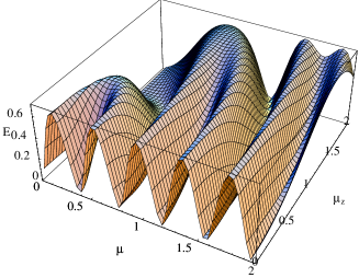
Figure 1: (Color online) Entanglement generated by the hamiltonian of the example 1 for the input state $|01\rangle$ as a function of the parameters $\mu,\mu_{z}$.

Example 1.– The non-degenerate Hamiltonian we consider is the following

$$H_{0}=\lambda_{1}\sigma_{z}\otimes\openone+\lambda_{2}\openone\otimes\sigma_{z},\quad(\lambda_{1}\neq\lambda_{2})$$ (6)

The eigenvectors are given by the standard product basis. We introduce the family of unitaries $U(\mu,\mu_{z})=\exp[iK(\mu,\mu_{z})]$ where

$$K(\mu,\mu_{z}):=\mu\sigma^{+}\otimes\sigma^{-}+\bar{\mu}\sigma^{-}\otimes\sigma^{+}+\mu_{z}(\sigma_{z}\otimes\openone-\openone\otimes\sigma_{z})$$ (7)

and the associated iso-spectral family $H(\mu,\mu_{z}):=U(\mu,\mu_{z})H_{0}U(\mu,\mu_{z})^{\dagger}.$ The Hilbert space is given by ${\cal H}={\rm span}\left\{|00\rangle,|01\rangle,|10\rangle,|11\rangle\right\}$ and we can split it in the two subspaces ${\cal H}_{0}={\rm span}\left\{|00\rangle,|11\rangle\right\}$ and ${\cal H}_{1}={\rm span}\left\{|01\rangle,|10\rangle\right\}$, where obviously ${\cal H}={\cal H}_{0}\oplus{\cal H}_{1}$.

The evolution operator $U$ is the identity on ${\cal H}_{0}$ while it is a straightforward exercise to verify that on ${\cal H}_{1}$ it yields: $U|01\rangle\equiv|\xi\rangle\equiv a|01\rangle+b|10\rangle$ and $U|10\rangle\equiv|\zeta\rangle\equiv-\overline{b}|01\rangle+\overline{a}|10\rangle$, where $a=\cos\theta+\frac{2i\sin\theta}{\theta}\mu_{z}$, $b=\frac{4i\sin\theta}{\theta}\overline{\mu}$ and $\vec{\theta}\equiv 2(\mu+\overline{\mu},i(\mu-\overline{\mu}),\mu_{z})$. For the generic state $|\Psi\rangle=\alpha|01\rangle+\beta|10\rangle+\gamma|00\rangle+\delta|11\rangle$ one has $C^{2}=\left|xy-\gamma\delta\right|^{2},$ where $x=\alpha a-\beta\overline{b}$ and $y=\alpha b+\beta\overline{a}$.

For $|01\rangle$ the evolved state is $\left|\xi\right\rangle=a|01\rangle+b|10\rangle$ and its reduced density matrix is obviously $\rho=\rm{diag}(\left|a\right|^{2},\left|b\right|^{2})$ whose eigenvalues are $\left|a\right|^{2}$ and $1-\left|a\right|^{2}$. The condition to obtain a maximally entangled state is hence $\left|a\right|^{2}=\frac{1}{2}$, that is, $\sin^{2}\theta=\frac{1}{2}\left[1+\left(\frac{\mu_{z}}{2\left|\mu\right|}\right)^{2}\right]$. This equation admits (at least) one solution iff $\left|\mu_{z}\right|\leq 2\left|\mu\right|.$ Thus a maximally entangled state can be reached starting from either $|01\rangle,|10\rangle.$ In Fig. 1 is showed the reachable entanglement from the input state $|01\rangle$ as a function of the parameters $\mu,\mu_{z}.$ We see how moving in the parameter space to higher values of $\mu_{z}$ spoils the reachibility of a maximally entangled state.

Example 2.– Let us examine now the following unitary family: $U=\exp(i\sum_{j=1}^{3}\lambda_{j}\sigma_{j}\otimes\sigma_{j})$ In the so-called magic basis $[|\Psi_{1}\rangle=({|00\rangle+|11\rangle})/\sqrt{2},|\Psi_{2}\rangle=-i(|00\rangle-|11\rangle)/\sqrt{2},|\Psi_{3}\rangle=(|01\rangle-|10\rangle)/\sqrt{2},|\Psi_{4}\rangle=-i(|01\rangle+|10\rangle)/\sqrt{2}]$ (as well in the Bell basis) these unitaries are diagonal and read $U=\sum_{k=1}^{4}e^{ih_{k}}|\Psi_{k}\rangle\langle\Psi_{k}|$ where $\{h_{1}=\lambda_{1}-\lambda_{2}+\lambda_{3},h_{2}=\lambda_{1}+\lambda_{2}-\lambda_{3},h_{3}=-\lambda_{1}+\lambda_{2}+\lambda_{3},h_{4}=-\lambda_{1}-\lambda_{2}-\lambda_{3}\}.$ So in this basis the input state is $|\Psi\rangle=\sum_{k}w_{k}|\Psi_{k}\rangle$ and the output state is $|\Phi\rangle=\sum_{k}w_{k}e^{-ih_{k}}|\Psi_{k}\rangle.$ The concurrence is given by $C^{2}=\sum_{k,l}(w_{k}e^{-ih_{k}})^{2}(w^{*}_{l}e^{ih_{l}})^{2}$. Following Ref kc , we find that the maximum reachable concurrence is $C=\max_{k,l}|\sin(h_{k}-h_{l})|$ and the product input state which gives the best entangling capability as a function of the parameters $\lambda_{k}$ is then $\frac{1}{\sqrt{2}}(|\Psi_{k}\rangle+i|\Psi_{l}\rangle).$ So for instance a maximally entangled state can be reached from the input state $\frac{1}{\sqrt{2}}(|\Psi_{1}\rangle+i|\Psi_{2}\rangle)=|00\rangle$ for parameters such that $\lambda_{3}-\lambda_{2}=\pi/4$ (see Fig. 2).

Before passing to the conclusions we would like to show that the first two-qubit Hamiltonian family associated with the unitaries (7) can be used to generate a non trivial entangling gate in an adiabatic fashion.

Proposition 3 An adiabatic loop in the parameter space $(\mu,\mu_{z})\,(|\mu|^{2}+\mu_{z}^{2}=\mbox{const})$ gives rise to the diagonal unitary mapping $|\alpha\beta\rangle\rightarrow\exp(i\phi_{\alpha\beta})|\alpha\beta\rangle$ where, if $\gamma$ denotes the geometric contribution , $E_{\alpha\beta}$ the eigenvelues and $T$ is the operation time, one has $\phi_{01}=E_{01}\,T+\gamma,\,\phi_{10}=E_{01}\,T-\gamma,\,\phi_{00}=E_{00}\,T,\,\phi_{11}=E_{11}\,T$ For $\phi_{01}+\phi_{10}-(\phi_{00}+\phi_{11})=-4\,T\neq 0\mbox{mod}\,2\pi$ the obtained transformation is equivalent to a controlled-phase-shift.

Proof. Indeed it is easy to check that i) by the adiabatic theorem the evolution has to be diagonal in the product basis ii) the geometric contribution of the states $|\alpha\alpha\rangle\,(\alpha=0,1)$ is zero ($\Leftarrow U(\mu,\mu_{z})|\alpha\alpha\rangle=|\alpha\alpha\rangle$) iii) In the one-qubit subspace spanned by $|{\bf{0}}\rangle:=|01\rangle$ and $|{\bf{1}}\rangle:=|10\rangle$ the unitaries $e^{iK}$ with the $K$ defined in (7) look like $U(\mu,\mu_{z})=exp[i(\mu\tilde{\sigma}^{+}+\bar{\mu}\tilde{\sigma}^{-}+\mu_{z}\tilde{\sigma}_{z})].$ This latter equation can be of course written as ${\bf{B}}\cdot\dot{\bf{\sigma}}$ where a fictious magnetic field ${\bf{B}}$ has been introduced. One can then use the standard Berry-phase argument for a spin $1/2$ particle in an adiabatically changing magnetic field to claim that under a ${\bf{B}}$ going along an adiabatic loop, one has $|{\bf{0}}\rangle\mapsto e^{i\gamma}|{\bf{0}}\rangle$ and $|{\bf{1}}\rangle\mapsto e^{-i\gamma}|{\bf{1}}\rangle$. Here $\gamma$ denotes the standard geometric phase i.e., proportional to the solid angle swept by ${\bf{B}}.$ The final equivalence claim stems from a known result in literature calarco . $\hfill\Box$

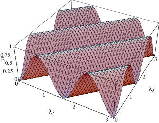
Figure 2: (Color online) Entanglement for the unitary $U=e^{i\sum_{i=1}^{3}\lambda_{i}\sigma^{i}\otimes\sigma^{i}}$, with the input state $\frac{1}{\sqrt{2}}(|\Psi_{1}\rangle+i|\Psi_{2}\rangle)$ as a function of $\lambda_{2},\lambda_{3}$, with $\lambda_{1}=1$.

Of course the general fact that entangling gates can be obtained via adiabatic manipulations is not new see e.g.,HQC ekert . The point of Prop 4. is to show explicitly how the particular two-qubit Hamiltonian family associated to the untarries (7) can be exploited for enacting controlled phase via a simple adiabatic protocol.

V Conclusions.

In this paper we analyzed the entanglement generation capabilities of a parametric family of adiabatically connected non-degenerate Hamiltonians. One prepares the system in a separable eigenstate of of a distinguished Hamiltonian $H_{0}$ in the family and then the space of parameters is adiabatically explored. The system remains then in an energy eigenstate and the (bi-partite) entanglement contained in such an eiegenstate can be maximized over the manifold of control parameters. We introduced an associated measure $e$ of adiabatic entangling power and discussed its properties and relations with a previously introduced measure for the case of iso-spectral families of Hamiltonians. We illustrated the general ideas by studying explicitly the adiabatic entangling power of concrete two-qubits Hamiltonian families. We also showed how to generate a non-trivial two-qubits entangling gate by means of adiabatic loops.

We thank M. C. Abbati, A. Manià, L. Faoro and an anonymous referee for useful comments. P.Z. gratefully acknowledges financial support by Cambridge-MIT Institute Limited and by the European Union project TOPQIP (Contract IST-2001-39215)

References

- (1) D.P. DiVincenzo and C. Bennett, Nature 404, 247 (2000)
- (2) E. Farhi et al, Science 292, 472 (2001)
- (3) Wim van Dam, M. Mosca, U. Vazirani, quant-ph/0206003
- (4) D. Aharonov, A. Ts-Shma, quant-ph/0301023
- (5) A. Messiah, Quantum mechanics, John Wiley and Sons (1958)
- (6) A. Jones et al. , Nature 403, 869 (2000); G. Falci et al. , Nature 407, 355 (2000).
- (7) M.V. Berry, Proc. R. Soc. Lond. A 392, 45 (1984)
- (8) P. Zanardi and M. Rasetti, Phys. Lett. A 264, 94 (1999); J. Pachos, P. Zanardi and M. Rasetti, Phys. Rev.A 61, 010305(R) (2000); L.-M. Duan,J. I. Cirac and P. Zoller, Science 292, 1695 (2001)
- (9) Unanyan et al, Phys. Rev. Lett. 87, 137902 (2001); S. Gu rin et al, Phys. Rev. A 66, 032311 (2002); R. G. Unanyan et al, Phys. Rev. A 66, 042101 (2002) R. G. Unanyan, M. Fleischhauer, quant-ph/0208144;
- (10) U. Dorner et al, Phys. Rev. Lett 91, 073601 (2003)
- (11) P.W. Anderson, Concepts in Solids: Lectures on the Theory of Solids (World Scientific Lecture Notes in Physics , Vol 58)
- (12) A. Osterloh et al, Nature (London) 416, 608 (2002); T. J. Osborne, M. A. Nielsen, Phys. Rev. A 66, 032110 (2002) G. Vidal et al, Phys. Rev. Lett. 90, 227902 (2003)
- (13) Here we are assuming, without loss of generality, that Ker
- (14) W. Dür et al, Phys. Rev. Lett 87, 137901 (2000)
- (15) P. Zanardi et al, Phys. Rev A, 62 030301(R) (2000)
- (16) B. Krauss, I. Cirac, Phys. Rev. A 63, 062309 (2001)
- (17) Ekert et al, J. Mod. Opt. 47, 2501 (2000))
- (18) See appendix B.1 of T. Calarco, I. Cirac, P. Zoller, Phys. Rev. A 63, 62304 (2001)