Quantum Error Correction in Globally Controlled Arrays

Abstract

An interesting concept in quantum computation is that of global control (GC), where there is no need to manipulate qubits individually. It is known that one can implement a universal set of quantum gates on a one-dimensional array purely via signals that target the entire structure indiscriminately. But large-scale quantum computation requires more than this: one must be able to perform efficient error correction, which has requirements in terms of noise level, time, space (scaling) and in particular parallelism. Keeping in mind these requirements, we prove GC can support error-correction, by implementing two simple codes. We discuss the issues involved in extending our approach to full fault-tolerant computation with this type of architecture.

Typical proposals for a solid-state quantum computation (QC) demand a precise control of both the individual constituent qubits and the interactions between them. The Kane scheme Kane is an archetypal example: in all such approaches one is required to switch individual interactions ‘on’ and ‘off’. An alternative is the idea of global control lloyd ; Controlunit ; SimonB ; SimonB.2 ; SimonB.2003 . In this approach, it is not necessary to individually address qubits. Instead one applies global signals, e.g. laser pulses, to the entire structure indiscriminately. With a suitable arrangement of qubits within the array, it is then possible to discover a sequence of such signals which have a net effect only at the desired points (i.e. only affecting specific qubits).

From an experimental standpoint, there are obvious advantages to such an approach. It can simplify the device structure, removing the need to have control elements (e.g. metallic electrodes) directed to each and every qubit. Moreover, in many otherwise promising QIP candidates, such as molecular scale structures, is it simply impossible to ‘plumb in’ qubit specific control elements. The global control paradigm may be the only option in such cases. Furthermore, even in rare cases where there is no technical obstacle to fabricating multiple control elements, there remains the issue that each such element is a potential decoherence source, typically ‘dangerously’ close to the qubits.

Lloyd’s original GC model lloyd ; Controlunit involved a one-dimensional array of cells, each being a two-state system coupled to its nearest neighbors with an Ising type interaction. Lloyd employed a regular pattern of three cell types, $ABCABC...$, where each type has a distinct transition energy. He demonstrated that one can perform a universal set of gates with this type of structure, noting that only the cell on the end need be independently controlled. Subsequently, Benjamin SimonB demonstrated that the same type of result can be achieved with only two types of cells, $ABABAB..$, and without the need to distinguish between the neighbors of a cell. More recently Benjamin has extended the approach to systems with Heisenberg interactions, initially assuming that interaction strengths can be collectively switched SimonB.2 , and subsequently dispensing with this condition SimonB.2003 ; SimonPreP .

In all these variants, there are costs associated with adopting the global control principle. Most obviously, they each employ an encoding that associates several physical (pseudo-)spins with each logical qubit. There is also a corresponding need for each logical gate operation to be rendered into several global pulses. The severity of these space/time costs increases as we consider systems with lower complexity (e.g. fewer cell types) or systems over which we have less control (e.g. no ability to switch interactions, even collectively). For one extreme case, namely a one-dimensional array of two alternating cell types with ‘always-on’ Ising interactions SimonB , the best known encoding requires at least eight physical spins for each logical qubit. However, a more profound cost is the loss of parallelism, as we discuss later.

The criteria for successful quantum error correction (QEC) Shor ; Steane3 and fault-tolerant computation Steane2 have been established in considerable detail. Steane Steane1 and others have shown that besides the basic per qubit error rate, factors like time (number of steps), space (e.g. the number of qubits used) and in particular the level of parallelism (number of logic gates performed simultaneously in the same computational step) must be considered as well. It is known that one-dimensional structures with nearest neighbor interactions can support QEC Ben-Or2 , but the issue of parallelism is crucial. Aharonov and Ben-Or Ben-Or have employed an elegant analysis to prove that, in the presence of noise (error rate per quantum logic gate) QC requires a degree of parallelism which is better than logarithmic in device size. Their argument involved excluding classes of quantum system than can be simulated efficiently on a classical device, and which, therefore, are not interesting as quantum computers. So, it is a fundamental requirement that this level of parallelism should be exceeded in order to perform new quantum algorithms which are actually infeasible classically. Here we argue that, within certain reasonable assumptions, globally controlled architectures can implement error correction with a degree of parallelism that scales linearly with system size – thus exceeding their condition.

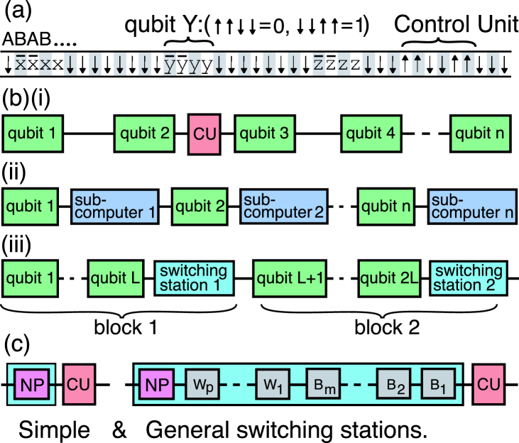
Figure 1: (a) The encoding of qubits and the control unit, following the scheme in Ref. SimonB . (b)(i) Serial model with a single control unit (b)(ii) Parallel model using ‘subcomputer’, enabling access to individual qubits (b)(iii) Model optimized for error correction, with one ‘switching station’ (SS) for each of the $M$ blocks. (c) The general SS includes $m={\rm Log}_{2}(M)$ label bits, a few ‘working’ bits, and a CU.

Our approach is suitable for all the schemes of Refs lloyd ; Controlunit ; SimonB ; SimonB.2 ; SimonB.2003 ; SimonPreP . When we wish explicitly to count the numbers of steps, etc, we will employ the scheme in Ref. SimonB (depicted in Fig. 1(a)). All the schemes share a common tactic to localize quantum operations to one point (and hence one qubit) within the device despite the constraint that all control signals are sent indiscriminately to the entire structure. They employ a ‘control unit’ (CU) - not a physical device but rather a local pattern of states which (in the simplest schemes) occurs in only one place along the device. With an appropriate choice of representation for the qubits and for the CU, it is possible to find sequences of updates to perform a ‘toolbox’ of basic functions:

1. A sequence whose net effect is to move the CU with respect to the qubits, without disrupting those qubits. Then we can position our unique CU pattern anywhere within the set of qubits.

2. A sequence which has the net effect of transforming the qubit nearest to the CU, but no net effect on any other qubit. This allows single qubit gates to be implemented.

3. A third sequence, the least trivial to derive, which implements a gate operation as the CU moves back and forth between two qubits.

For initial state preparation and eventual readout, we may assume that the cell on one end of the device is independently controllable and readable (perhaps by being physically coupled to additional devices). Alternatively, we might perform readout by exploiting a dissipative decay, as mentioned later in connection with qubit erasure.

It is important to stress that the CU is a classical set of definite 0’s and 1’s (except when it is actively involved in performing a quantum gate, as described above). Therefore, one can employ a relatively crude form of error prevention for the CU - for example SimonB we can cause the state of CU to collapse (effectively, to measure it) when we wish. This is important since an error in the CU pattern itself could be catastrophic to the scheme - much as a bit flip in program memory of a conventional computer could cause a crash. If a CU bit acquires a small element of superposition, due to a slightly imperfect EM pulse for example, a subsequent projection onto the 0/1 basis will recover the correct state with high probability. This can be thought of as a low level “Zeno” type of error correction zenoEffect . We can illustrate the idea with the following observation: in the scheme of Ref.SimonB , at times other than when a gate is actively being applied, it should never be the case that a ‘lone’ $|1\rangle$, i.e. a $|1\rangle$ with both neighbors as $|0\rangle$, exists anywhere on the device. Then we are free to frequently send pulses that have the effect, “If you are in state $|1\rangle$ and your neighbors are both $|0\rangle$, then dissipatively reset to $|0\rangle$”. Such measures can stabilize against bit-flips; since the CU is a classical state, it is an eigenstate of the Z operator and is thus already tolerant of phase-flips.

With this simple approach our device has become purely sequential, since updates have a net effect only at the location of the CU (Fig. 1(b)(i)). The obvious way to try and recover some degree of parallelism is to have numerous CU’s present at different locations. Since a parallel algorithm will involve varying distributions of simultaneous gates, we must somehow create/destroy CUs. Doing so directly by external intervention would require local control, so we must instead find a way to effectively disable a CU by processes internal to the device. Benjamin SimonB proposed an elaborate scheme for doing so, which indeed recovers a high degree of parallelism: for a device containing $N$ basic qubits one introduces $N$ CUs, and $N$ uniquely labelled regions called ‘sub-computers’ to enable/disable those CUs (Fig. 1(b)(ii)). This interesting idea suffers from the high number of additional cells required. Each qubit would need $\lceil{\rm log}_{2}(N)\rceil$ label bits along with a number, $R$, of auxiliary bits. Taking account of the spacing, which doubles the number of cells needed, we have $2*4*(\lceil{\rm log}_{2}(N)\rceil+R)+10$ cells needed for each subcomputer+CU+qubit. A device containing 80,000 cells, which in the simple architecture could support 10,000 qubits, can now support fewer than 900 qubits.

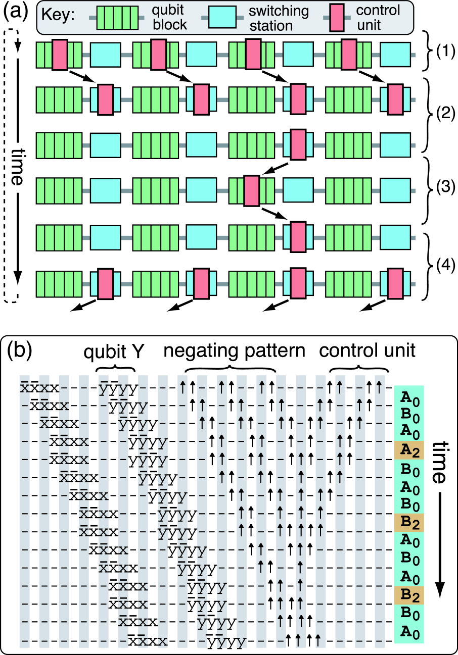
Figure 2: Upper: Schematic showing the process of alternating between the error correction phase (1) and the algorithmic phase (3). This involves switching ‘off’ (2) the majority of the CUs, and subsequently switching them back ‘on’ (4). Lower: One possible means of effectively ‘deactivating’ a CU. Here the SS is simply a binary pattern occupying 10 cells, denoted “negating pattern” in this figure (here dashes denote cells in state $|\downarrow\rangle$). In response to the update sequence shown on the right, the CU is ‘absorbed’ into the pattern. Note that if all the updates $A_{2}$ and $B_{2}$ were omitted, then the CU would pass transparently through. We have designed this process for the scheme introduced in Ref.SimonB , but procedures for the other GC schemes can be similarly obtained.

We propose a less costly process, related to this ‘sub-computer’ idea but optimized to produce a form of parallelism that is useful for QEC. We describe the process in detail for simple (non-concatenated) codes and then discuss an extension to fault tolerant scenarios. The basic concept is to exploit the fact that typical codes (such as the Steane [[7,1,3]] code, or the Shor [[9,1,3]] code) involve representing each “computational qubit” by encoding it into a block of $L$ adjacent basic qubits. Suppose that our device contains $N$ basic qubits (each possibly requiring several cells for its representation), and these basic qubits are used to represent a smaller number $M$ of encoded qubits. For simplicity of exposition, we assume that each encoded qubit corresponds to a distinct block, although this is not a requirement. During the error correction process, we will have $M$ CUs active in the entire device (Fig. 1(b)(iii)), one for each block simToLloyd . Note that the size of a block itself remains constant once the QEC code has been chosen, the number of adjacent qubits used to encode each computational qubit being the same for all of them. The number of computational qubits then scales linearly with the size of the array. More importantly, the number of pulses needed to perform any particular operation during the QEC process is independent of the actual array size, as the movement of the CU stays confined within each block of constant size (depicted in Fig. 3).

In this way, as we will discuss, we can correct all $M$ encoded qubits in constant time, independent of $M$. We then ‘switch off’ the majority of these CUs – in the simplest scheme, all but one. This reduced subset of CUs is used to perform step(s) of the actual quantum algorithm (a Shor factorization, say), before reactivating all $M$ CUs for another error correction cycle (Fig. 2(a)). The process of activating and deactivating the CUs takes place in regions which we will call ‘switching stations’ (SS) to differentiate from the more costly ‘sub-computers’ in Benjamin’s earlier proposal.

It may be helpful to note that during the periods when we are moving CUs around (eg the first three pulses in Fig. 2(b)), each pulse moves the CU though a distance of one unit - we are discretely ‘clocking’ the motion. (In fact, because Fig. 2 employs the particular scheme of RefSimonB , the qubits also necessarily move one unit in the opposite direction, so their separation is reduced by two units per pulse, but for clarity we simply speak of the CUs moving to their targets). The discrete, rather than ballistic, motion of these of these entities allows us to ‘choreograph’ the motion of complex processes, involving multiple qubits approaching multiple targets, without needing to be concerned about different entities meeting at slightly different times.

Consider first the simple case where we wish to switch between $M$ CUs in the device, and just one CU. This can be done with relatively little cost, either in time or cell count. Each SS occupies a small number of cells at the right side (say) of each $L$ qubit block, as shown in Fig. 2(a). All but one of the SS are identical: each contains a pattern of states that has the property that it will absorb, or deactivate, a CU when suitable global pulses are applied (Fig 2(b)). Relative to the CU, this pattern stays in the SS area and then can be viewed as static, like the qubits. The process must be reversible so that a CU is emitted, or reactivated, when the inverse sequence is applied. The remaining SS is exceptional: it does not act in this way and, in fact, it can simply be an empty region of the array. Thus when each of the $M$ CUs passes through the corresponding SS it will be deactivated - except for the CU passing though the ‘empty’ SS.

The details of exactly how the SS causes a deactivation of a CU will depend on the exact scheme. For completeness, we briefly describe some options relevant to the particular scheme of Ref. SimonB . The simple method mentioned above is to literally remove the CU from the device by using the ‘negating pattern’ shown in Fig. 2. Alternatively one could delay the CU, causing it to fail to ‘arrive’ at the target qubit SimonB . A third possibility, perhaps the most conceptually elegant, would exploit the fact that the scheme can easily implement gates with multiple control qubits (such as Control-Control-NOT for example). One would employ a single bit in the SS and use this bit as the control qubit in a conditional gate. Thus, an unconditional single qubit gate $G$ in the logical algorithm would become a Control-$G$ with the SS as the controlling bit, and similarly a Control-NOT would be implemented as a Control-Control-NOT, etc.

Having removed all but one of the CUs, we can now proceed to perform any manipulation we wish with the single remaining CU. In fact we will perform the next step of the overall quantum algorithm (a Shor factorization task, we have supposed). It will only be possible to perform a certain number of steps before it becomes necessary to apply another error correction cycle: then we simply apply the reverse of the deactivation process to recover all $M$ CUs. Ideally we would wish to have at least enough time between error correction cycles to perform an arbitrary two-qubit gate between remote qubits. Because we are assuming a 1D array with nearest neighbor interaction, the time required for this scales with $N$ - thus for a very large device one might not be able to complete such a gate. In this case one could resort to performing a series of swaps, after successive EC cycles, to bring the qubits closer.

Within each error correction phase, the $M$ active CUs are each associated with one of the $M$ encoding blocks (Fig. 2(a) step 1). They simultaneously perform the same series of qubit operations within each block to implement the EC code (Fig. 3). Recalling that each block is also of constant size (for simple EC), and that $M$ is linearly proportional to the device size, we conclude that we need only apply a fixed number of pulses to accomplish the error correction over the entire device. That is, we achieve the ideal of linearly scaling parallelism which of course exceeds the condition on parallelism mentioned above.

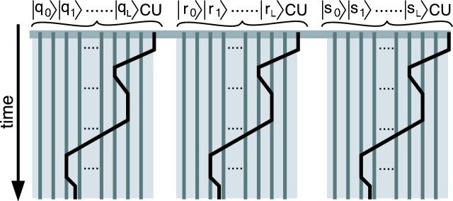
Figure 3: Schematic of the block encoding process. In response to global pulses, each Control Unit (black lines) simultaneously performs the operations of the QEC within a multi-qubit block that encodes a given logical qubit ($q$, $r$, $s$). The white areas correspond to the qubits left for spacing and the Switching Stations.

Our global pulses necessarily cause exactly the same behavior within each block, whereas the errors (if any) that occur in each block will vary. However, this can be dealt with by internalizing the process of applying the ‘fix’ within the EC algorithm. Let us consider the quantum state $|Q_{P}\rangle$ of an encoded block, subject to decoherence from the environment. Such decoherence can always Nielsen be characterized by the X (bit-flip) or Z (phase-flip) types of error, or a combination of the two (Y$\equiv$ZX). In the following lines we neglect normalization for the sake of clarity. Note that a ‘collapse’ to a specific state of the environment can occur at any time without altering the result. The general process of interaction with the environment takes the initial state $|Q_{P}\rangle|E_{0}\rangle$ to

$$|Q_{P}\rangle|E_{0}\rangle+\delta_{X}|Q_{X}\rangle|E_{1}\rangle+\delta_{Y}|Q_{Y}\rangle|E_{2}\rangle+\delta_{Z}|Q_{Z}\rangle|E_{3}\rangle$$

At the beginning of the error correction process we introduce ancilla qubits, initially all in state $|0\rangle$, onto which the error syndrome is placed. This results in a particular auxiliary state for each of the different error types:

$$|Q_{P}\rangle|E_{0}\rangle|A_{0}\rangle+\ \ \ \ \ \ \ \ \ \ \ \ \ \ \ \ \ \ \ \ \ \ \ \ \ \ \ \ \ \ \ \ \ \ \ \ \ \ \ \ \ \ \ \ \ \ \ \ \ \ \ \ \ \$$

$$\delta_{X}|Q_{X}\rangle|E_{1}\rangle|A_{1}\rangle+\delta_{Y}|Q_{Y}\rangle|E_{2}\rangle|A_{2}\rangle+\delta_{Z}|Q_{Z}\rangle|E_{3}\rangle|A_{3}\rangle$$

The circuits we are using here apply a specific correction conditional on the error syndrome given by the ancilla qubits. The original state is then recovered for each type of error syndrome:

$$|Q_{P}\rangle\left(|E_{0}\rangle|A_{0}\rangle+\delta_{X}|E_{1}\rangle|A_{1}\rangle+\delta_{Y}|E_{2}\rangle|A_{2}\rangle+\delta_{Z}|E_{3}\rangle|A_{3}\rangle\right)$$

Subsequently the ancilla qubits are erased back to $|0\rangle$, making them available for another syndrome extraction. There is thus no need for a syndrome ‘measurement’ in the commonly described sense Nielsen .

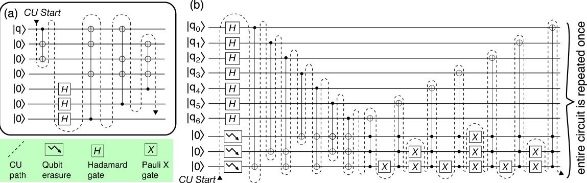
Figure 4: Encoding (a) and EC circuits (b) for the Steane [[7,1,3]] code. The computational qubits of the circuits are in the same order, from top to bottom, as they are on the cell chain from right to left (c.f. Figs. 1 & 2). EC involves syndrome extraction and subsequent correction for both phase-flip and bit-flip errors. The movement of the CU back-and-forth through the array is indicated by the dashed line.

The behavior of the CU within a given block is shown explicitly in Figs. 4 and 5 for the Steane [[7,1,3]] code and the Shor [[9,1,3]]. These simple (non-fault tolerant) QECCs each correct a single error. The movement of the CU is indicated in order to show the importance of finding an efficient route. To formally minimize the path of the CU, one would need to specify the complexity of the various types of gate, which depends on the particular physical model lloyd ; Controlunit ; SimonB ; SimonB.2 ; SimonB.2003 .

Due to its movement through the block, the CU could be seen as potentially dangerous for the scheme if it carries any error, as this could be propagated to all the qubits. Here we should stress again the importance of the CU being a classical pattern of states, which makes it much more resilient to errors in that we can use dissipation to stabilize it. Thus we would aim to achieve a degree of stability in the CU more akin to that of conventional bits rather than qubits. Additionally, for the particular encoding scheme we have adopted here SimonB , there is a strong sense in which the CU moves transparently through the intervening qubits: this transparency is not ‘constructed’ by performing swap operations, for example, but occurs ‘naturally’ as the CU and qubit collide under the simple driving sequence (pulses $A_{0},B_{0},A_{0},B_{0}...$). There is minimal interaction between the CU and any qubits passed, and consequently the risk of error propagation via the CU is also minimized.

In these simple circuits, and in more complex fault-tolerant procedures, it is crucially important to be able to reset (erase) qubits. Here we assume that this can be achieved by a mechanism analogous to the one proposed in Ref. SimonB for efficient measurement. We envisage that at least one of the cell ‘types’ has an unstable third state $|\rightsquigarrow\rangle$, which rapidly decays to the ground state. Then we can initiate an erasure via a special form of one-qubit gate operation (symbolized by an arrow in the circuits, Fig. 4 and 5) using:

$\mathbf{U}=\begin{pmatrix}0&0&1\\ \vskip 6.0pt plus 2.0pt minus 2.0pt\cr 0&1&0\\ \vskip 6.0pt plus 2.0pt minus 2.0pt\cr 1&0&0\\ \end{pmatrix}$ in the basis {$\downarrow$, $\uparrow$, $\rightsquigarrow$}.

The use of such auxiliary state(s) could potentially introduce problems of ‘leakage’ out of the computational subspace. In order to negate this risk, the third state must be chosen to be in a very distinct energy level, separated from the qubit states by an energy gap that prevents any spontaneous jump of the quantum states to this level. This state can then only be reached by a precise manipulation via the quantum logic gate U. As a physical example, one might consider the qubit states as the eigenstates of an electron spin in a quantum dot (or molecule) while the transient state is an optically excited state (e.g. an exciton) that can only be reached from one of the spin states due to Pauli blocking pazy . Such a state would decay extremely rapidly, and could not be “acidentally” excited by ambient thermal excitations, even at room temperature.

A physical process such as this will allow erasure of the ancilla qubits after the error syndrome has been successfully used to correct a bit/phase error (see for example rightmost of Fig. 5 (i)). Once reset to the ground state, they can be used again within a given EC process, thus reducing the total number of auxiliary qubits required per block. Figures 4 and 5 both include optimizations of this kind.

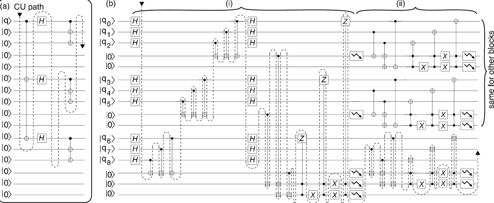
Figure 5: Encoding (a) and EC circuits (b) for the Shor [[9,1,3]] code. Phase-flip errors are resolved in section (i), and bit-flip errors in (ii). The notation is as defined in the key in Fig. 4.

In Table 1 we make a comparison of the efficiency of the two codes illustrated in Figs. 4 and 5. However we should emphasize that the scheme we describe here is completely independent of the size of the chosen EC code, and then perfectly scalable to more complex or simpler ones. Indeed it would be highly desirable from an experimental perspective to start with a much simpler model of code (simply correcting bit-flip errors for example) to demonstrate the feasibility of implementing the basic scheme. For the explicit pulse count, we assume the physical model in Ref. SimonB , since this is the ‘worst case’ in the number of cells per qubit. To get an idea of the time scale of a correcting process, the table gives a calculation of the number of pulses needed to perform all the quantum operations of each circuit, within one encoding block and with one CU. Erasure can be considered here as a particular one-qubit gate operation.

Table 1: Characteristic figures for the number of primitive global pulses needed for error-correction, for each of the two codes implemented.

Correction step	Steane [[7,1,3]]	Shor [[9,1,3]]
Encoding	464	397
Syndrome measur./recovery	3622	2955
Total	4086	3352

With the inclusion of the ancilla qubits, the Steane code is encoded on blocks of 10 qubits (requiring 80 cells), and the Shor code on blocks of 16 qubits (128 cells). A simple sketch of the global movement of the CU through the array is described in each circuit, designed to minimize its movements between the different gates. We must stress that the circuit design and the movement of the CU are not aggressively optimized for minimum pulse count - there are improvements that can ‘shave off’ a few pulses at the cost that the circuits become more cumbersome to illustrate. Therefore the figures in the Table should be regarded as characteristic rather than definitive. In Appendix II we make some remarks to illustrate the counting process that we employed. The Table shows a modest speedup of about 20 percent in favor of the Shor code, which is balanced by the fact this code needs more qubits per block to be implemented.

In the scheme described above, we switch between $M$ CUs for the error correcting phase, and just one CU for the algorithm phase (Fig. 2(a)). This allowed us to use trivially simple switching stations, that unconditionally deactivate, or reactivate, a CU (Figs. 1(b)(iii) & 2(b)). Consequently each SS can be a fixed small size, and they require a constant proportion of the entire device as it scales. In this respect the scheme is efficient: it does not require significant additional spatial resources versus the basic global control scheme. However, in another sense it is inefficient: during the algorithm phase we have only a single CU at our disposal, and therefore our potentially parallel device is acting as a purely serial computer. We can reach a better compromise between spatial and temporal efficiency by introducing a specialized form of the ‘labels’ concept mentioned in Ref. SimonB . Now each SS gains a binary label which we can exploit to differentiate it from neighboring stations (Fig. 1(c)). In the strong limit of using unique labels, this therefore requires Order($M{\rm Log}_{2}(M)$) additional cells in total (although shorter, repeating labels can be useful, as we demonstrate in Appendix I). The process of switching from the error correcting phase to the algorithmic phase is now less trivial, although the actual error correcting phase is not affected at all by the labelling. We apply a sequence of global pulses that causes each of the $M$ CUs to simultaneously move to a SS, and there to perform a small computation ${\bf C}$. The computation applied in each SS is of course identical, being driven by the same pulses, but the data on which the computation acts, i.e. the binary label, is unique. Therefore the outcome of the computation will vary from one SS to the next. This outcome is a binary variable represented by either altering, or not altering, the pattern of states responsible for (de)activating the CU. Then when the CU subsequently moves through this region (c.f. Fig 2(b)), it may or may not be deactivated, depending on ${\bf C}$ and the label of that SS. In this way we can switch from all $M$ CUs being active during the error correction phase, to some chosen subset of all $M$ CUs in the algorithmic phase. This is illustrated in Figure 6. Note that the time $\tau$ associated with the label computation must be less than O($N$) otherwise it would have been quicker to perform the parallel gates in series. One could not enable/disable a completely arbitrary sub-set of the $M$ CUs under this time constraint patExist , so our procedure does not efficiently implement a completely general arrangement of gates. However, there are a great many useful distributions of CUs which do correspond to fast $\tau$. Two examples are discussed in Appendix I.

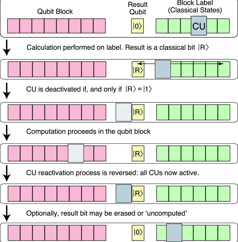
Figure 6: This is a schematic representation of a single block of qubits and their switching station, incorporating the idea of a classical label of states to identify the switching station, so that an algorithm can be run to selectively enable/disable a subset of the CUs.

We now discuss some of the issues involved in extending the above ideas to fully fault tolerant (FT) processing. The above arguments have demonstrated that a high degree of parallelism can be harnessed for EC; in fact this parallelism can also be optimally exploited for operating on concatenated codes. In Appendix I we give some explicit examples of how this can be achieved. We conclude, therefore, that 1D globally controlled structures can achieve adequate parallelism for FT processing. However a second issue is that of performing operations between encoded blocks in a robust way. Typically fault–tolerant implementation of such a gate involves performing a measurement over multiple qubits and applying an operation depending on the result Nielsen . To formally establish fault tolerance, it is necessary to show how to ‘internalise’ such operations with an algorithm, in much the same way as syndrome extraction and correction was performed with an algorithm. Fortunately Aharonov and Ben-Or have indeed shown (Theorem 4 of Ben-Or2 ) how to perform these gates for a subset of CSS codes. Importantly, they use only operations which are standard elements of computation, and require only the additional ability of adding and discarding qubits, which is equivalent to the qubit erasure process that we have described. As one might expect, operating without the measurement process increases the overhead in terms of the number of ancillas required and apparently results in a more severe error threshold (although it is emphasized that their result is not optimal). Hence, for a suitable choice of error correcting code, a globally controlled architecture not only has sufficient parallelism to allow fault tolerant quantum computation (which in turn allows a quantum algorithm to be run to arbitrary accuracy), but has known techniques that detail exactly how to perform such operations.

It is important to stress, however, that the CU must behave very reliably if is not to be an “Achilles’ heel” in an FT implementation. If a permanent error were to occur on a CU, then this could be catastrophic for the calculation since this would not only affect a single qubit in one level of concatenation, but would also affect every other level. However, as has already been noted, the CUs are classical states and can thus be stabilised against decoherence, e.g. by dissipation, more simply and effectively than quantum states can. We note that a temporary error in a CU would be less of a problem. In the worst case, a single encoded qubit at a given level of concatenation acquires an error. The QECC of the next level of concatenation can correct for this single error (once the error has been removed from the CU). Nevertheless, one must regard an error in the CU as being as potentially destructive as a bit error in the program of a conventional computer. Thus, in physical systems where the CU cannot be sufficiently stabilized (for example, any system in which flip errors are a dominant source of noise) the route to FT processing which we outline here would not be suitable. It is an interesting question whether some variant of the CU idea can be conceived, within which one could immediately detect and correct CU errors. This is perhaps a direction for future work.

The authors would like to thank Andrew Steane for useful conversations. This work was supported by the EPSRC and the DTI under the foresight LINK project. SCB acknowledges the support of the Royal Society.

Appendix I

Here we demonstrate the potential use of the ‘labelled switching station’ idea by describing two particularly interesting arrangements of control units, both of which are relevant to fault tolerant computation with so-called concatenated codes. In such codes the QECC is applied recursively to ‘encode the codes’, possibly through multiple levels. The first arrangement we discuss is the fundamental pattern for such processing, i.e. a pattern of one CU per block, where that block may now consist of a hierarchy of lesser blocks. The second pattern is a local group of CUs suitable for performing efficient ‘bit wise’ operations on encoded blocks, without decoding them.

For the basic, non-fault tolerant EC scenario described in the body of the paper, we were able to switch between a single CU and a CU for every block of qubits. Such a block consists of $L$ computational qubits (including the necessary ancillas, but not including the SS). Now however we wish to be able to choose whether we have a single CU or a CU every $L^{i}$ SSs, where $i$ denotes the level of concatenation of error correcting code ($i\geq 0$). This will be possible if we place a (non-unique) classical label in the region of each SS when initialising the quantum computer. Let us assume that we intend to use a total of $p-1$ levels of concatenation of our QECCs. Then the number stored in the label of the $i^{th}$ SS is given by the prescription

$$SS_{i}=\sum_{j=1}^{p-1}R(i\text{ mod }L^{j})$$

where the function $R(x)$ returns 1 if $x=1$ and 0 otherwise. The number $p$ is specially reserved to only be at a single location, which would otherwise have contained a $p-1$ label – this will facilitate switching to a single CU when necessary. We emphasise that the above expression is not a calculation that is run on the quantum computer, it simply defines the label arrangement which is placed in regions of the computer during initialization. These states are then exploited during the subsequent computation.

Recalling that the algorithm is, at all times, ‘sent in’ by global pulses, at a given moment during error correction we will be operating at a certain level of the concatenation, say the $b^{\rm th}$ level, throughout the device. To switch on a CU every $L^{b}$ SSs ($0\leq b\leq p-1$), we just run a program that returns 0 if the value of the label is less than $b$ and 1 otherwise. The result of this then determines whether or not to ‘deactivate’ a CU at that SS location. Earlier we discussed the various means by which a CU can be effectively deactivated. For the present discussion it is convenient to assume we are employing the third mechanism we outlined, namely making a single bit in the SS act as a control bit in subsequent qubit gates. We shall denote the number stored in the SS label by $a$, and the $x^{th}$ most significant bit of the number by $a_{x}$. Fig. 7 shows how to implement a suitable algorithm using ancillas, $c$ (which we regard as part of the label space). The binary label itself will be stored on $\log_{2}(p)$ bits and, given the qubit erasure process, $U$, then we only require 2 ancillas. We only require $O(\log_{2}(p))$ steps in the program to decide which CUs activate/deactivate (given that the program will run on every SS simultaneously). Recall that $p$ characterizes the total number of levels of encoding and therefore it must be a modest number in any plausible device – thus our running time of $O(\log_{2}(p))$ is very fast. The result of this algorithmic test of the label is the single classical ‘outcome’ bit in each SS, denoted by $r$ in Fig. 7. The algorithm shown in that figure is a general procedure that will work for any $b$. For specific $b$ it should be possible to customize the algorithm, making it yet more efficient.

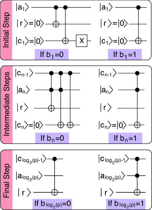
Figure 7: Algorithm to implement a set of CUs suitable for fault tolerant concatenated codes, as described in the text. The symbol $a_{x}$ represents the $x^{th}$ most significant bit of the number stored in the label. $r$ contains the result of the computation on the label. The bits $c$ are the ancillas that mark whether we have a subsequent recursion, and thus act as a control in the next step.

The method presented here can be adapted to different patterns of CUs, by organising the numbers stored in the SSs differently. The only requirement is that there exists a hierarchy in the patterns of CUs such that, to switch between one pattern and another requires either the activation or deactivation of a subset of CUs, not both. We shall therefore use the same algorithm for the second desirable arrangement of control units, which we now discuss. Suppose we were able to activate and deactivate not just a single CU in a block, but some form of super-CU, a dense local patterning of control units capable of performing efficient bitwise operations on a single encoded qubit, and acting on all the constituent qubits simultaneously. For example, in the encoding shown in Fig. 5, this would mean leaving on 9 CUs, in the pattern of 3 on, 2 off, 3 on, 2 off, 3 on (nothing needs to be done to the ancillas). To generate this pattern at the level of individual qubits, we would need to provide a SS for every such qubit, so in fact it would be inefficient to implement this for a basic QECC. However, for concatenated codes, we can make use of the idea without additional resources.

We aim to create a single super-CU for each level of concatenation above the lowest. To do this, we set the labels on the switching stations equal to

$$SS_{i}=p-\sum_{j=1}^{p-1}\delta(i\leq L^{j})\prod_{k=1}^{j-1}R^{\prime}(i\text{ mod }L^{k},k)$$

where, in the case of the Shor code of figure 5, $L=16$ and $R^{\prime}(x,k)$ returns $1$ for $1+r\times L^{k-1}\leq x\leq(r+3)\times L^{k-1}$, where $r\in\{0,5,10\}$. Note that since we have no super-CU at the lowest level of concatenation, each operation would need to be repeated 9 times, starting on the unencoded qubits $1,2,3,6,7,8,11,12,13$ each time. (This is however a small cost compared to the dramatic device size increase that would be required for a SS for each qubit.) The prescription for $SS_{i}$ is of the form $p-f(i)$ because we now want to activate CUs as we go up the levels of concatenation, instead of deactivating them as we did in the previous example. Note that when we are computing on an encoded qubit, we also have to act on encoded ancillas (section 5.4 of Ben-Or2 ), so the 3-2-3-2-3 pattern of the Shor code needs to be carried over to all levels of concatenation.

We might also like to be able to manifest a repeating pattern of these super-CUs across the device, but such a pattern is not consistent with the requirements for the algorithm of Fig. 7. That is not to say that such an algorithm doesn’t exist. Any single pattern of CUs for concatenated codes can always be realised in a SS with $p$ qubits. The $i^{th}$ qubit simply indicates whether or not that particular SS should be switched on or off in the $i^{th}$ level of concatenation. This only takes up a constant proportion of the device size, and does not require a computation to be performed on the SS. Whether any encoding is possible should then be obvious from the ‘missing’ numbers. If all the numbers from 0 to $2^{p}-1$ are present on different labels, then, obviously, no encoding of the labels will be able to store the required information more efficiently.

We cannot perform all operations in a bitwise fashion and so we also need to retain the ability to switch to the control of a single CU every $L^{i}$ SSs, and to having only a single CU. This is trivial to do, since all we need to do is have two labels (combining to form a single, larger label), using the two systems of label patterning already specified. Depending on what type of state we desire, we choose which half of the pattern to perform the algorithm on.

The discussion in this Appendix has simply highlighted two of the many possible uses of the labelled-SS concept. We hope that these examples suffice to show that the idea is a powerful one.

Appendix II

Here we make a few remarks to illustrate the counting method that we employed to obtain the pulse totals quoted in the Table. Recall that we are adopting the scheme of Ref. SimonB since this is the ‘worst case’ in terms of size costs (a consequence of the extreme simplicity of the $ABAB$ model). We distinguish the “approach pulses”, which only move the CU from being adjacent to one qubit to being adjacent to another, from the “operation pulses” which modify the state of the qubit. For example, for a one-qubit logic gate, starting from the stage where a CU is next to the target qubit a total of 15 pulses are required: 8 pulses to perform the operation followed by the first 7 in reverse order to restore the CU pattern. In the case of a controlled operation between, say, the first (control) and the fourth (target) qubit, starting from a CU next to the control qubit, 5 pulses are needed for the CU to interact with the control. Several “approach pulses” (2*4) follow to bring the CU next to the target. Then 9 pulses are needed to perform the operation, and we reapply the first 8 pulses in reverse order as before. We must then reapply the earlier pulses (approach+ encoding) in reverse to complete the process of restoring the CU to its original form. However, it is efficient to retain the altered form of the CU if several qubits are subject to the same control qubit: one can then move directly to those other targets. The circuits are designed to employ this optimization wherever possible.

References

- (1) B. Kane, Nature 393, 133 (1998).
- (2) Seth Lloyd, Science 261, 1569 (1993).
- (3) Seth Lloyd, preprint http:xxx.lanl.gov/:quant-ph/9912086
- (4) S. C. Benjamin, Physical Review A 61, 020301 (2000).
- (5) S. C. Benjamin, Physical Review Letters, 88, 017904 (2002).
- (6) S. C. Benjamin and S. Bose, Phys. Rev. Lett. 90 247901 (2003).
- (7) S. C. Benjamin, B. Lovett and J. H. Reina, preprint http://xxx.lanl.gov/quant-ph/0407063.
- (8) A.R. Calderbank and P.W. Shor, Physical Review A 54, 1098 (1996).
- (9) A.M. Steane, Proc. Roy. Soc. Lond. A 452, 2551 (1996).
- (10) A. M. Steane, preprint http://xxx.lanl.gov/quant-ph/9809054.
- (11) A. M. Steane, preprint http://xxx.lanl.gov/quant-ph/9708021.
- (12) D. Aharonov and M. Ben-Or, preprint http://xxx.lanl.gov/quant-ph/9906129.
- (13) D. Aharonov and M. Ben-Or, preprint http://xxx.lanl.gov/quant-ph/9611029.
- (14) P. Facchi at al, Phys. Rev. Lett. 86 2699 (2001).
- (15) This is in fact reminiscent of an idea presented by Lloyd in his original work on these structures Controlunit , but here we applying it to the specific issue of QEC.
- (16) Quantum Computation and Quantum Information M. A. Nielsen and I. L. Chuang, Cambridge University Press 2000.
- (17) There must be patterns of CUs which cannot be produced using a sequence of less than O() updates, given that the number of distinct updates is limited. Otherwise we would have a means of compressing arbitrary bits, corresponding to the enabled/disabled CUs, into less than O(N) symbols.
- (18) E. Pazy et al Europhys. Lett. 62, 175 (2003).
- (19) Quantum Computing, J. Gruska, McGraw-Hill 1999.