Phase-space approach to the study of decoherence in quantum walks

Abstract

We analyze the quantum walk on a cycle using discrete Wigner functions as a way to represent the states and the evolution of the walker. The method provides some insight on the nature of the interference effects that make quantum and classical walks different. We also study the behavior of the system when the quantum coin carried by the walker interacts with an environment. We show that for this system quantum coherence is robust for initially delocalized states of the walker. The use of phase-space representation enables us to develop an intuitive description of the nature of the decoherence process in this system.

I Introduction

Quantum walks Kempe have been proposed as potentially useful components of quantum algorithms Aharonov . In recent years these systems have been studied in detail and some progress has been made in developing new quantum algorithms using either continuous ChildsExp or discrete ShenviExp versions of quantum walks. The key to the potential success of quantum walks seems to rely on the ability of the quantum walker to efficiently spread over a graph (a network of sites) in a way that is much faster than any algorithm based on classical coin tosses.

Quantum interference plays an important role in quantum walks being the crucial ingredient enabling a faster than classical spread. For this reason, some effort was made in recent years in trying to understand the implications of the process of decoherence for quantum walks KendonDec ; BrunOct ; KendonJan . Decoherence, an essential ingredient to understand the quantum–classical transition DecoRef , could turn the quantum walk into an algorithm as inefficient as its classical counterpart. The models studied in this context can be divided in two classes depending on how the coupling with an external environment is introduced. In fact, a quantum walk consists of a quantum particle that can occupy a discrete set of points on a lattice. In the discrete version, the walker carries a quantum coin, which in the simplest case can be taken as a spin-$1/2$ degree of freedom. The algorithm proceeds so that the walker moves in one of two possible directions depending on the state of the spin (for more complex regular arrays, a higher spin is required). So, in this context it is natural to consider some decoherence models where the spin is coupled to the environment and others where the position of the walker is directly coupled to external degrees of freedom. The specific system in which the algorithm is implemented in practice will dictate which of these two scenarios is more relevant. Several experimental proposals to implement discrete quantum walks in systems such as ion traps Travaglione , cavity QED cavityQED , and optical lattices Dur have been analyzed (see also Ref. Du for a recent NMR implementation of a continuous quantum walk).

The main effect of decoherence on quantum walks is rather intuitive: as the interaction with the environment washes out quantum interference effects, it restores some aspects of the classical behavior. For example, it has been shown that the spread of the decohered walker becomes diffusion dominated proceeding slower than in the pure quantum case. This result was obtained both for models with decoherence in the coin and in the position of the walker KendonDec ; BrunOct ; KendonJan . However, it is known that classical correspondence in these systems has some surprising features. For example, for models with some decoherence in the quantum coin the asymptotic dispersion of the walker grows diffusively but with a rate that does not coincide with the classical one BrunOct . Also, a small amount of decoherence seems to be useful to achieve a quantum walk with a significant speedup KendonDec ; KendonJan .

In this work we will revisit the quantum walk on a cycle (and on a line) considering models where the quantum coin interacts with an environment. The aim of our work is twofold. First we will use phase-space distributions (i.e., discrete Wigner functions) to represent the quantum state of the walker. The use of such distributions in the context of quantum computation has been proposed in Ref. MPS02 , where some general features about the behavior of quantum algorithms in phase space were noticed. A phase-space representation is natural in the case of quantum walks, where both position and momentum play a natural role. Our second goal is to study the true nature of the transition from quantum to classical in this kind of model. We will show that models where the environment is coupled to the coin are not able to induce a complete transition to classicality. This is a consequence of the fact that the preferred observable selected by the environment is the momentum of the walker. This observable, which is the generator of discrete translations in position, plays the role of the “pointer observable” of the system DecoRef ; Zurek81 . Therefore, as we will see, the interaction with the environment being very efficient in suppressing interference between pointer states preserves the quantum interference between superpositions of eigenstates of the conjugate observable to momentum (i.e., position). Again, the use of phase-space representation of quantum states will be helpful in developing an intuitive picture of the effect of decoherence in this context. The paper is organized as follows: In Sec. II we review some basic aspects of the quantum walk on the cycle. We also introduce there the phase-space representation of quantum states for the quantum walk and discuss some of the main properties of the discrete Wigner functions for this system. In Sec. III we introduce a simple decoherence model and show the main consequences on the quantum walk algorithm. In Sec. IV we present a summary and our conclusions.

II Quantum walks and their phase-space representation

II.1 Quantum walks on the cycle

The quantum walks on an infinite line or in a cycle with $N$ sites are simple enough systems to be exactly solvable. For the infinite line the exact solution was presented in Ref. Nayak . The case of the cycle was first solved in Ref. Aharonov . However, the exact expressions are involved enough to require numerical evaluation to study their main features. Here we will review the main properties of this system presenting them in a way which prepares the ground to use phase-space representation for quantum states (we will focus on the case of a cycle, the results for the line can be recovered from ours with $t\leq N$).

For a quantum walk in a cycle of $N$ sites, the Hilbert space is $\mathcal{H}=\mathcal{H}_{N}\otimes\mathcal{H}_{2}$, where $\mathcal{H}_{N}$ is the space of states of the walker (an $N$-dimensional Hilbert space) and $\mathcal{H}_{2}$ is the two–dimensional Hilbert space of the quantum coin (a spin $1/2$). The algorithm is defined by a unitary evolution operator which is the iteration of the following map:

$$\mathcal{U}_{walk}=U^{\sigma_{z}}\ H.$$ (1)

Here $H$ is the Hadamard operator acting on the Hilbert space of the quantum coin [$H=(\sigma_{x}+\sigma_{z})/\sqrt{2}$, $\sigma_{i}$ being the usual $2\times 2$ Pauli matrices]. The operator $U$ is the cyclic translation operator for the walker, which in the position basis is defined as $U|n\rangle=|n+1\rangle$ (mod $N$). It is worth stressing that the operator $U^{\sigma_{z}}$ is nothing but a spin–controlled translation acting as $U^{\sigma_{z}}|n\rangle\otimes|{0\atop 1}\rangle=|n\pm 1\rangle\otimes|{0\atop 1}\rangle$. So, the map $\mathcal{U}_{walk}$ consists of a spin–controlled translation preceded by a coin toss, which is implemented by the Hadamard operation (the use of the Hadamard operator in this context is not essential and can be replaced by almost any unitary operator on the coin Kempe ).

The notion of phase-space is natural in the context of this kind of quantum walk. In fact, the position eigenstates $\{|n\rangle,\ n=0,\ \ldots,\ N-1\}$ form a basis of the walkers’ Hilbert space $\mathcal{H}_{N}$. The conjugate basis is the so–called momentum basis $\{|k\rangle,\ k=0,\ \ldots,\ N-1\}$. Position and momentum bases are related by the discrete Fourier transform, i.e.,

$$\langle n|k\rangle={1\over\sqrt{N}}\exp(2\pi ink/N).$$ (2)

The cyclic translation operator $U$ that plays a central role in the quantum walk is diagonal in momentum basis since $U|k\rangle=\exp(-i2\pi k/N)|k\rangle$. This simply indicates that momentum is nothing but the generator of finite translations. As a consequence of this, the total unitary operator defining the quantum walk algorithm is also diagonal in such basis. This fact, which was noticed before by several authors, enables a simple exact solution of the quantum walk dynamics. Indeed, we can write the initial state of the system using the momentum basis of the walker as (below $\rho$ denotes the total density matrix of the system formed by the walker and the coin)

$$\rho(0)=\sum_{k,k^{\prime}=0}^{N-1}c_{k,k^{\prime}}|k\rangle\langle k^{\prime}|\otimes\rho_{2}(0),$$ (3)

where $\rho_{2}(0)$ is the initial state of the quantum coin (we assume that the initial state of the combined system is a product, but this assumption can be relaxed). After $t$ iterations of the quantum map the reduced density matrix of the walker (denoted as $\rho_{w}$) is

$$\rho_{w}(t)=\sum_{k,k^{\prime}=0}^{N-1}c_{k,k^{\prime}}f(k,k^{\prime},t)\ |k\rangle\langle k^{\prime}|,$$ (4)

$$f(k,k^{\prime},t)={\rm Tr}_{2}[M_{k}^{t}\rho_{2}(0){M_{k^{\prime}}^{\dagger}}^{t}],$$ (5)

where the operator $M_{k}$ is defined as

$$M_{k}=\exp(-i2\pi\ k\sigma_{z}/N)\ H.$$ (6)

All the temporal dependence is contained in the function $f(k,k^{\prime},t)$ which can be exactly computed in a straightforward way: One should first expand the initial state $\rho_{2}(0)$ in a (nonorthogonal) basis of operators of the form $|\phi^{l}_{k}\rangle\langle\phi^{m}_{k^{\prime}}|$ ($l,m=1,2$), where $|\phi_{k}^{l}\rangle$ are the eigenstates of the operator $M_{k}$ (i.e., $M_{k}|\phi_{k}^{l}\rangle=\lambda_{k,l}|\phi_{k}^{l}\rangle$). The explicit expressions for the eigenstates $|\phi_{k}^{l}\rangle$ and the eigenvalues $\lambda_{k,l}$ will not be given here since they can be found in the literature (see, for example, Nayak ). After doing this the evolution of the quantum state is fully determined by the equation

$$f(k,k^{\prime},t)=\sum_{l,m=1,2}(\lambda_{k,l}\lambda^{*}_{k^{\prime},m})^{t}\ \langle\phi^{l}_{k}|\rho_{2}(0)|\phi^{m}_{k^{\prime}}\rangle\ \langle\phi^{m}_{k^{\prime}}|\phi^{l}_{k}\rangle.$$ (7)

Below we will describe the properties of this solution using a phase-space representation for the quantum state of the system.

II.2 Phase-space representation

Wigner functions Wigner are a powerful tool to represent the state and the evolution of a quantum system. For systems with a finite-dimensional Hilbert space, the discrete version of Wigner functions was introduced using different methods (see Ref. Wigner-Discrete ). We will follow the approach and notation used in Ref. MPS02 , where these phase-space distributions were applied to study properties of quantum algorithms. For completeness, we will give here the necessary definitions and outline some of the most remarkable properties of the discrete Wigner functions.

For a system with an $N$-dimensional Hilbert space the discrete Wigner function can be defined as the components of the density matrix in a basis of operators defined as

$$A(q,p)=U^{q}RV^{-p}\exp(i\pi pq/N).$$ (8)

These are the so–called phase-space point operators. They are defined in terms of the cyclic shift $U$ (which in the position basis acts as $U|n\rangle=|n+1\rangle$), the reflection operator $R$ (which in the position basis acts as $R|n\rangle=|-n\rangle$), and the momentum shift $V$ (which generates cyclic displacements in the momentum basis, i.e., $V|k\rangle=|k+1\rangle$). Phase-space operators are unitary, Hermitian and form a complete orthogonal basis of the space of operators (they are orthogonal in the Hilbert–Schmidt inner product since they satisfy that ${\rm Tr}[A(q,p)A(q^{\prime},p^{\prime})]=N\delta_{q,q^{\prime}}\delta_{p,p^{\prime}}$). Expanding the quantum state in the $A(q,p)$ basis as

$$\rho=\sum_{q,p=0}^{N-1}W(q,p)A(q,p),$$ (9)

the coefficients $W(q,p)$ are the discrete Wigner functions of the quantum state, which are obtained as

$$W(q,p)={1\over N}{\rm Tr}[\rho A(q,p)].$$ (10)

This function has three remarkable properties that almost give it the status of a probability distribution. The first two properties are evident: Wigner functions are real numbers (a consequence of the Hermiticity of the phase-space operators) and they provide a complete description of the quantum state (a consequence of the completeness of the basis of such operators). The third property is less obvious: marginal probability distributions can be obtained by adding values of the Wigner function along lines in phase-space. For this to be possible, it turns out that the phase-space has to be defined as a grid of $2N\times 2N$ points where $W(q,p)$ is given at each point precisely by Eq. (10). Thus, adding the values of the Wigner function over all points satisfying the condition $aq-bp=c$ one gets the probability to detect an eigenstate of the operator $D(b,a)=U^{b}V^{a}\exp(i\pi ab/N)$ with eigenvalue $\exp(i\pi c/2N)$ (the sum is equal to zero if such eigenvalue does not exist). In particular, adding the Wigner function along vertical lines $q=c$ one obtains the probability to detect eigenstates of the operator $D(0,1)=V$, with eigenvalues given by $\exp(i\pi c/2N)$. These numbers are equal to zero if $c$ is odd and they are equal to the probability for measuring the position eigenstate $|c/2\rangle$ when $c$ is even. Complementary, adding values of the Wigner function along horizontal lines enables us to compute the probability to detect a momentum eigenstate.

A final remark about properties of the discrete Wigner function is in order. Figure 1 shows the Wigner function of a position eigenstate $|n_{0}\rangle$ and of a superposition of two position eigenstates, such as $(|n_{1}\rangle+|n_{2}\rangle)/\sqrt{2}$. As we see, in the first case the function is positive on a vertical line located at $q=2n_{0}$ and is oscillatory on a vertical line located at $q=2n_{0}+N$. The interpretation of these oscillations is clear. It is well known that Wigner functions display oscillatory regions whenever there is interference between two pieces of a wave packet. In this case, the cyclic boundary conditions we are imposing (that originate from the fact that $U$ and $V$ are cyclic shift operators) generate a mirror image for every phase-space point. Thus, the oscillating strip can be interpreted as the interference between the positive strip and its mirror image. For the case of a quantum state which is a superposition of two position eigenstates, we observe two positive vertical lines with the usual interference fringes in between them. All these vertical lines have their corresponding oscillatory counterparts originated from the boundary conditions which are located at a distance $N$. In what follows we will show Wigner functions for typical states of a quantum walker.

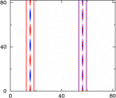
Figure 1: Wigner functions $W(q,p)$ for a localized state (up) and for a delocalized superposition state (down). The dimension of the Hilbert space is $N=41$. The horizontal (vertical) axis corresponds to position (momentum). Color code is such that red (blue) regions correspond to positive (negative) values while white corresponds to zero ($n_{0}=8$, $n_{1}=6$, $n_{2}=9$).

 

For an initial state where the walker starts at a given position and the spin is initially unbiased [$|\psi(0)\rangle_{2}=(|0\rangle+i|1\rangle)/\sqrt{2}$], the behavior of the quantum walker starts to deviate from its classical counterpart at early times (in this paper we will only consider unbiased initial states for the quantum coin). The phase-space representation of the state is shown in Fig. 3 and makes evident that a peculiar pattern of quantum interference fringes develops between the different pieces of the wave packet. The consequence of these interference effect is evident also when one looks at the probability distribution for different positions. This distribution is shown in Fig. 2 and has been previously studied in the literature (see Dur ; Nayak ; BrunOct ; KendonDec ). Like its classical counterpart, at a given time $t$ the state initially located at $n_{0}$ has support only on states $n$ satisfying that $n+t+n_{0}$ adds up to an even number. However, in general the quantum distribution differs from the classical one, exhibiting peaks located at $n=\pm t/\sqrt{2}$ and a plateau of height $1/\sqrt{2}t$ around $n_{0}$. After some time the Wigner function of the quantum walker develops a shape that resembles a thread, as it is clear in the pictures. For this reason we will call this a thread state.

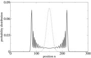
Figure 2: Probability distribution in position after $t=100$ iterations for an initially localized walker with unbiased spin. $N=301$, $n_{0}=150$. We only plot the function for sites such that $n+t+n_{0}$ adds to an even number (solid), and also include the classical distribution (dotted).

 

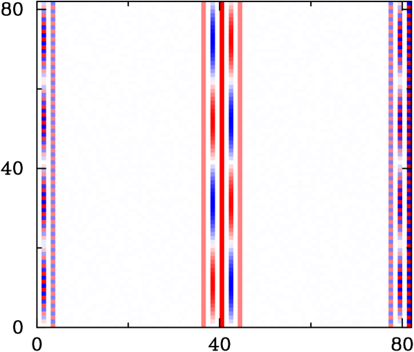
a) $t=2$

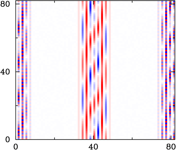
b) $t=4$

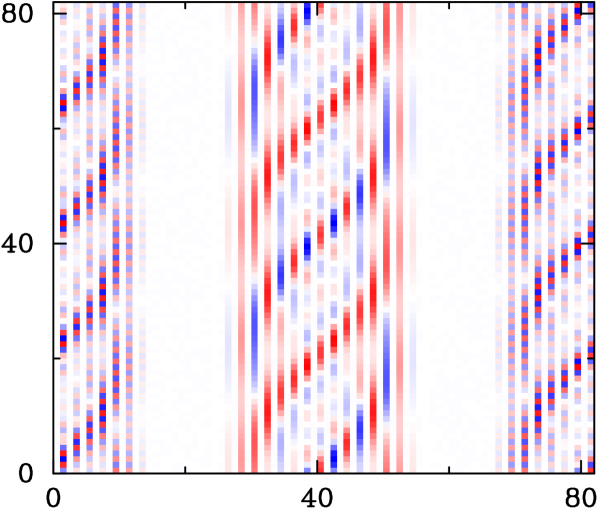
c) $t=8$

Figure 3: Discrete Wigner function $W(q,p)$ at different times. The initial state of the walker is localized at $n_{0}=20$ (the dimension of the Hilbert space is $N=41$). The quantum coin is in an unbiased initial state. Horizontal (vertical) axis corresponds to position (momentum).

 

It is also interesting to analyze the evolution of the quantum walk for delocalized initial states. In particular, we will consider an initial state that is a coherent superposition of two position eigenstates (whose Wigner function was already displayed in Fig. 1). We find a Wigner function that develops into a sum of two threads with a region in between where interference fringes are evident. This is displayed in Fig. 4. Some properties of the quantum walk for this kind of delocalized initial states were analyzed in Ref. Grudka where it was noticed that the asymptotic probability distribution can be rather different from the one obtained from a localized initial state. Below, we will show that the process of decoherence affects localized and delocalized initial states in a rather different way.

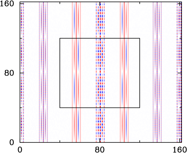
a) $t=2$

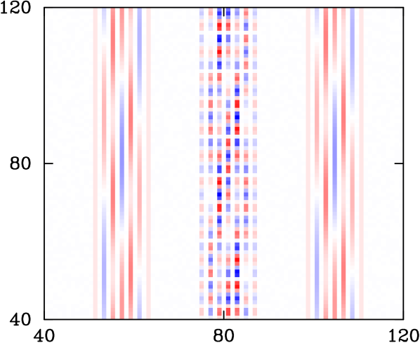
b) $t=3$

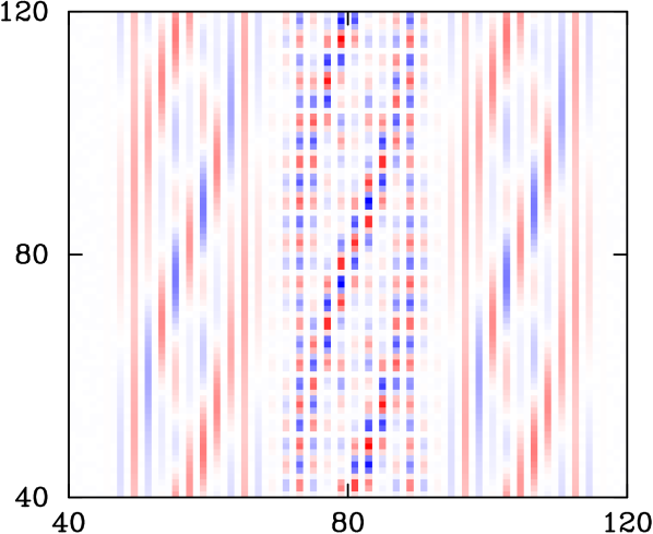
c) $t=6$

Figure 4: Discrete Wigner function $W(q,p)$ at different times, for an initial state of the walker which is a superposition of two position eigenstates ($N=81,\ n_{1}=28,\ n_{2}=52$) and an unbiased initial quantum coin. In (a) we plot the complete Wigner function (horizontal axis and vertical axis correspond to position and momentum, respectively). In (b) and (c) we only plot the Wigner function in the phase-space region defined by the black rectangle shown in (a). In this way the small scale oscillations of the Wigner function can be observed in detail.

 

III Decoherence and the transition from quantum to classical

III.1 The decoherence model

We will consider a quantum walk where the quantum coin couples to an environment. To describe such coupling we will use a model which was introduced and studied in detail in Ref. Teklemariam . In that paper it was shown that one can mimic the coupling to an external environment by a sequence of random rotations applied to the quantum coin, which have the effect of scrambling the spin polarization. More precisely, these kicks will be generated by the evolution operator

$$K_{j}=\exp(-i\epsilon_{j}\ \hat{n}\cdot\vec{\sigma}),$$ (11)

where the angles $\epsilon_{j}$ take random values and $\hat{n}$ is a fixed vector specifying the rotation axis. The virtue of this model is not only its simplicity but also the fact that can be experimentally implemented in a controllable manner using, for example, NMR techniques.

After the application of one step of the quantum walk algorithm and one kick the evolution of the total system is

$$\rho(t+1)=K_{j}\ U^{\sigma_{z}}H\ \rho(t)\ HU^{-\sigma_{z}}\ K_{j}^{\dagger},$$ (12)

To obtain a closed expression for the reduced density matrix of the walker for an ensemble of realizations of the random variables $\epsilon_{j}$ we follow the method proposed in Ref. Teklemariam (see Ref. BrunOct for a similar approach): Assuming that these angles are randomly distributed in an interval ($-\alpha$,$+\alpha$), this density matrix is

$$\rho_{w}(t) = {\rm Tr}_{2}[\int_{-\alpha}^{\alpha}{d\epsilon_{t}\over 2\alpha}\ldots\int_{-\alpha}^{\alpha}{d\epsilon_{1}\over 2\alpha}K_{t}U^{\sigma_{z}}H\ldots K_{1}U^{\sigma_{z}}H$$ (13)

$$\rho_{w}(0)\otimes\rho_{2}(0)\ HU^{-\sigma_{z}}K_{1}^{\dagger}\ldots HU^{-\sigma_{z}}K_{t}^{\dagger}]\$$

Expanding the initial state in the momentum basis as before enables us to simplify this expression. In fact, after doing this one can integrate over the random variables to find

$$\rho_{w}(t) = \sum_{k,k^{\prime}=0}^{N-1}c_{k,k^{\prime}}\tilde{f}_{n}(k,k^{\prime},t)|k\rangle\langle k^{\prime}|,$$ (14)

$$\tilde{f}_{n}(k,k^{\prime},t) = {\rm Tr}_{2}[O_{n}^{t}(\rho_{2}(0))].$$ (15)

Here $O_{n}$ is a superoperator acting on the spin state (depending on direction $\hat{n}$ of the kicks) as

$$O_{n}(\rho_{2}) = {(1+\gamma)\over 2}M_{k}\rho_{2}M_{k^{\prime}}^{\dagger}$$ (16)

$$+ {(1-\gamma)\over 2}\sigma_{n}M_{k}\rho_{2}M_{k^{\prime}}^{\dagger}\sigma_{n},$$

where $\gamma=\sin(2\alpha)/(2\alpha)$ is a parameter related to the strength of the noise (notice that $\gamma=1$ corresponds to unitary evolution, i.e., to $\alpha=0$). One can find a simple matrix representation for the superoperator $O_{n}$ for different choices of the rotation axis by writing $\rho_{2}(0)$ in the basis formed by the identity and the Pauli operators. In the Appendix we show the explicit form of this matrix representation, which is helpful in finding exact and numerical solutions to the problem. In what follows we will show results for the case $\hat{n}=\hat{y}$ (the other cases are qualitatively similar). To find the state of the walker at arbitrary times we simply need to find eigenstates and eigenvalues of the superoperator $O_{n}$. This can always be done numerically and also analytically in the interesting case of $\gamma=0$, which can be denoted as “total decoherence”. In such case, the exact solution turns out to be

$$\tilde{f}_{y}(k,k^{\prime},t) = \cos^{t}(2\pi(k-k^{\prime})/N)$$ (17)

$$\times \left(1-i\ p_{x}{\sin(2\pi(k-k^{\prime})/N)\over\cos(2\pi(k-k^{\prime})/N)}\right).$$

Several features of the decoherence effect are evident in the above formula. The environment produces a tendency towards diagonalization of the density matrix of the walker in the momentum basis (matrix elements with $k-k^{\prime}=N/4$ are maximally suppressed). The decay of nondiagonal elements is exponential in time, as already discussed in Ref. Teklemariam . It is also clear that momentum eigenstates are not affected by the interaction since they are eigenstates of the full evolution [in fact, from Eqs. (15) and (16) follows $\tilde{f}_{n}(k,k,t)=1$]. In this sense they are perfect pointer states for this model. In what follows we will present results concerning the evolution of several initial quantum states.

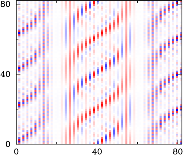
a) $\alpha=0.1$

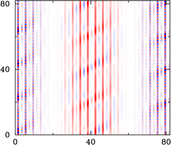
b) $\alpha=0.3\pi$

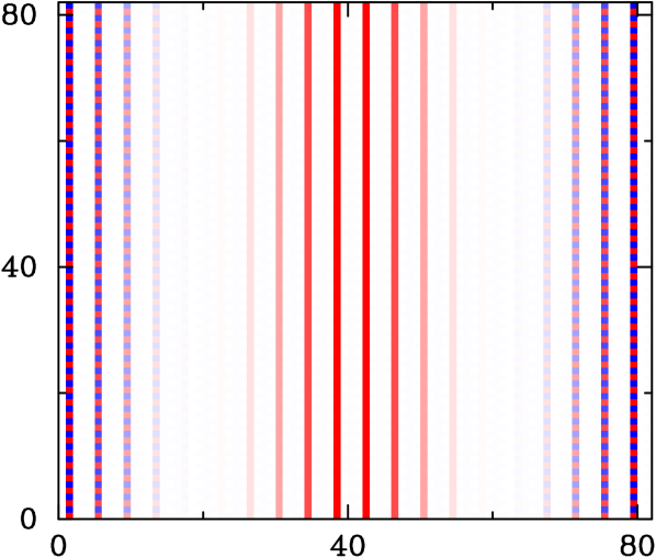
c) $\alpha=0.5\pi$

Figure 5: Discrete Wigner function $W(q,p)$ for a fixed time ($t=11$) and different values of the strength of the coupling to the environment ($\alpha$). The initial spin is in an unbiased state. Horizontal and vertical axis respectively correspond to position and momentum (total dimension of the Hilbert space is $N=41$ and the initial state is located at $n_{0}=20$).

 

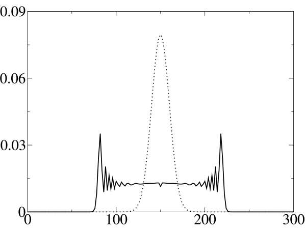
a) $\alpha=0.05\pi$

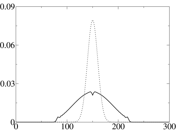
b) $\alpha=0.1\pi$

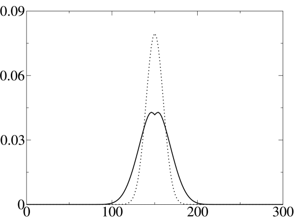
c) $\alpha=0.2\pi$

Figure 6: Probability distribution in position at $t=100$, for different values of the coupling to the environment (parametrized by $\alpha$). The initial state of the quantum coin is unbiased ($N=301$, $n_{0}=150$, and $\hat{n}=\hat{y}$). We only plot the function for sites such that $n+t+n_{0}$ adds to an even number (solid), and also include the classical distribution (dotted). Fig. 2 shows the same plot without decoherence.

 

III.2 Decoherence, pointer states, and the transition from quantum to classical

The effect of decoherence on the evolution of states which are initially localized in position has been analyzed elsewhere KendonDec ; KendonJan ; BrunOct . As shown in Fig. 5, the Wigner function of the evolved quantum state gradually loses its oscillatory nature. Thus, instead of a thread state the interaction with the environment gradually produces a mixed state with a binomial distribution in the position direction (which has an approximately Gaussian shape for large $t$) but remains constant along the momentum direction. It is worth noticing that for any value of $\gamma$ the resulting state has support only on position eigenstates satisfying that the sum $n_{0}+n+t$ is equal to an even number, as it was already pointed out for both the classical distribution ($\gamma=0$) and the purely quantum one ($\gamma=1$) in the preceding section. It is interesting to notice that the process of decoherence has a rather simple interpretation when represented in phase-space: Decoherence in phase-space is roughly equivalent to diffusion in the position direction. This is not unexpected: In fact, in ordinary quantum Brownian motion models a coupling to the environment through position (momentum) gives rise to a momentum (position) diffusion term in the evolution equation for the Wigner function. The situation here is quite similar, since the walker effectively couples with the environment through its momentum. This is indeed the case because the environment interacts with the quantum coin which is itself coupled with the walker through the displacement operator which is diagonal in the momentum basis. Therefore, the decoherence effect on the Wigner function is expected to correspond to diffusion along the position direction.

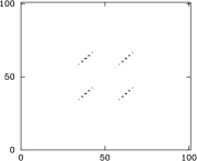
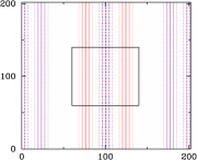
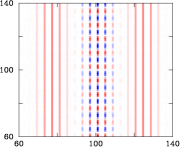
Figure 7: Absolute value of the density matrix in the position basis (left) and discrete Wigner function $W(q,p)$ (center) for a state evolving from an initially delocalized state of the quantum walker under full decoherence ($t=6$, $\alpha=0.5\pi$, $n_{1}=38$, $n_{2}=62$, $N=101$). The presence of quantum interference is manifested in the nondiagonal terms of the density matrix and in the oscillations of the Wigner function. The small scale oscillations of the Wigner function are shown in the right plot, which shows $W(q,p)$ in the phase-space region defined by the black rectangle depicted in the center plot.

 

As noticed before, if one considers initial states where the walker is localized in a well defined position, one can see that the probability distribution for the different positions of the walker gradually tends to the classical one by increasing the coupling strength $\alpha$ from $\alpha=0$ (no kicks) to $\alpha=\pi/2$. This is shown in Fig. 6.

From the above analysis we could be tempted to conclude that the interaction between the quantum coin and the environment induces the classicalization of the walker. However, this is not the case. The process of decoherence induced in this way is not complete. This is most clearly seen by analyzing how it is that the interaction with the environment affects initial states of the quantum walker which are not initially localized. In Fig. 7 we show the Wigner function of an initially delocalized state (shown in Fig. 1) under full decoherence. We can clearly see that decoherence does not erase all quantum interference effects. In fact, as mentioned above, the interaction with the environment induces diffusion along the position direction. Therefore, interference fringes which are aligned along the position direction are immune to decoherence. Thus, the final state one obtains from a superposition of two position eigenstates is not the mixture of two binomial states but a coherent superposition of them. This peculiar behavior is easily understood by noticing that this is a simple consequence of the fact that momentum eigenstates are pointer states: Decoherence is effective in destroying superpositions of pointer states but highly inefficient in destroying superpositions of eigenstates of the conjugate observable (position).

III.3 Entropy

By analyzing the entropy of the reduced density matrix of the walker one can get a more quantitative measure of the degree of decoherence achieved as a consequence of the interaction with the environment. For convenience we will not examine the von Neumann entropy $S_{V}$ but concentrate on the linear entropy defined as $S_{L}=-\ln({\rm Tr}[\rho_{w}^{2}])$, which is easier to calculate. This entropy provides a lower bound to $S_{V}$ entropy . It is possible to show that almost no entropy is produced by the decay of the coherence present in the initially delocalized superposition state. In fact, this can be seen by comparing the entropy produced from the initially delocalized superposition and the one originated from an initial state in which the walker is prepared in an equally weighted mixture of two positions. These entropies can be seen in Fig. 8. The initial entropy of the mixture is 1 bit [$\ln(2)$]. It is quite clear from the curves shown in such figure that the entropy arising from the initial mixture remains to be 1 bit higher than the one originated from the initial coherent superposition. Thus, the quantum coherence present in the initial state is robust under the interaction with the environment and does not decay at all.

Fig. 8 shows another interesting feature: One would naively expect a monotonic dependence of the entropy with the coupling to the environment (which is parametrized by $\alpha$). However this is not the case since the curves in Fig. 8 intersect. This peculiar effect is made more evident in Fig. 9 where we study the entropy at a fixed time as a function of the coupling strength. In this figure a clear indication of a nontrivial behavior is seen: For early times the entropy grows slowly with $\alpha$ and exhibits a flat plateau for large values of $\alpha$. However, as time progresses a peak develops: The largest value of entropy at a given time is not achieved by the largest coupling. To the contrary, the largest entropy is attained by an intermediate coupling $\alpha_{c}$, whose value decreases with time.

The fact that for a given time the maximal entropy is not achieved by the maximal coupling to the environment is counterintuitive. As entropy is a measure of the spread of a distribution, this strange behavior can be rephrased as a manifestation of the counterintuitive fact that the decohered state (which is approximately diagonal in position basis) has a probability distribution that is more spread for $\alpha=\alpha_{c}$ than for $\alpha>\alpha_{c}$. A possible explanation for this peculiar behavior is the following: For high values of the coupling to the environment the state rapidly becomes classical and the spread in position grows diffusively, as in the classical random walk. When the coupling to the environment is not strong, our result seems to indicate that the state of the walker remains “quantum” for a longer time during which it spreads at a rate faster than classical. When this quantum state finally decoheres it may end up having a larger entropy than the one attained for high coupling simply because it is spread over a wider range of positions. We speculate that there could be a relation between this peculiar feature and the properties that make some degree of decoherence useful for quantum walks as discussed by Kendon and Tregenna in KendonDec ; KendonJan . The value of the $\alpha_{c}$ introduced above depends on both $N$ and $t$ and could be related to the position of the minima reported in Refs. KendonDec ; KendonJan . For example, in a cycle regime ($t>>N$) $\alpha_{c}$ diminishes with increasing $N$ as it is also the case for the position of the minima of the so–called quantum mixing time Kempe ; KendonDec ; KendonJan .

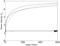
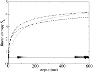
Figure 8: Linear entropy as a function of time for various values of the system–environment coupling strength: $\alpha=0$ (solid), $0.1\pi$ (dotted), $0.2\pi$ (dash dotted), $0.5\pi$ (dashed). The top (down) plot corresponds to an initial state which is an equally weighted mixture (superposition) of two position eigenstates. $N=401,\ n_{1}=150,\ n_{2}=250$.

 

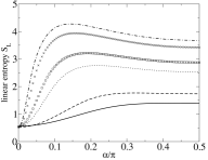
Figure 9: Linear entropy as a function of the coupling strength $\alpha$ for various values of time: $t=5$ (solid), $10$ (dashed), $50$ (dotted), $100$ ($\square$), $300$ ($\times$), $500$ (dash dotted). The initial state of the walker is well localized and the initial state of the quantum coin is unbiased. $N=401$ and all the curves are below the saturation regime [$\ln(N)\approx 5.994$]. It is evident that, after some time, the maximum value of the entropy is not achieved by the maximum value of the coupling strength.

 

IV Conclusions

The use of phase-space representation enables us to develop some intuition about the nature of the decoherence process in the kind of quantum walk analyzed in this paper. By coupling the quantum coin to an environment we obtain a decoherence model which is roughly equivalent to position diffusion. As we mentioned above, this is a natural result whose origin can be traced back to the way in which the system effectively couples to the environment (via the momentum operator). The relation between decoherence and position diffusion can also be established by analyzing in more detail the structure of the superoperator $O_{n}$ [given in Eq. (16)]. Let us consider the form of the superoperator after $t$ iterations. If we use Eq. (16) we can easily see that, as each iteration doubles the number of terms, we will have an expression with $2^{t}$ terms each one of which has Pauli operators applied at different times. To obtain the function $\tilde{f}_{n}(k,k^{\prime},t)$ one should compute the trace over the quantum coin. In each of the $2^{t}$ terms we can move the Pauli operator $\sigma_{n}$ towards the outside of the expression and cancel them due to the cyclic property of the trace. For the case $\hat{n}=\hat{y}$ it is easy to show that the only remaining effect of the Pauli operators (that in this case anti–commute with the Hadamard operator) is to reverse the direction of the rotation in $M_{k}$ defined in Eq. (6). The final expression can be shown to be

$${\rm Tr}(O_{y}^{t}(\rho)) = \sum_{\alpha_{t}=0,1}\ldots\sum_{\alpha_{1}=0,1}{1\over 2^{t}}\left(1+\gamma\right)^{t-\bar{\alpha}_{t}}\left(1-\gamma\right)^{\bar{\alpha}_{t}}$$ (18)

$$\times {\rm Tr}\left(M_{k_{t}}\ldots M_{k_{1}}\rho M_{k^{\prime}_{1}}^{\dagger}\ldots M_{k^{\prime}_{t}}^{\dagger}\right),$$

where $\bar{\alpha}_{j}=\alpha_{1}+\ldots+\alpha_{j}$ and $k_{j}=(-1)^{\bar{\alpha}_{j-1}}k$ (we use the convention $\bar{\alpha}_{0}\equiv 0$). Therefore, the superoperator is the sum of $2^{t}$ terms each one of which contains a contribution that is identical to that of a quantum walk where the direction of the walker is chosen at random after the first step. Each of the $2^{t}$ terms is labeled by a $t$–bit string $(\alpha_{1},\ldots,\alpha_{n})$ and corresponds to a quantum walk where the direction of the $j$th step ($j\geq 2$) is reversed if and only if $\bar{\alpha}_{j-1}$ is odd. In the limit of total decoherence each of these terms has equal weight. Therefore the final state is simply the average over an ensemble where each member corresponds to each of the $2^{t-1}$ possible choices of two directions (forward or backward) for the $t-1$ steps (notice that the direction of the first step is not affected by the decoherence model we chose). For this type of decoherence it is clear that the quantum walk becomes a random walk. The relation between decoherence and position diffusion is quite evident in this way. It is worth pointing out that similar models of decoherence were considered in Ref. Bianucci in a different context.

Other decoherence models have been analyzed for quantum walks KendonDec ; KendonJan ; Dur , where the effective coupling to the environment is through the position observable. In such case, we expect decoherence to correspond to diffusion along the momentum direction. Combining the two types of decoherence (i.e., considering coupling to the environment via the quantum coin and the position of the quantum walker) the initial state corresponding to a superposition of two positions would finally decay into a mixture of two binomial states (see Ref. Bianucci for similar results obtained when studying decoherence models with a natural phase-space representation in a finite quantum system evolving under various quantum maps).

The above conclusions are generic for any model in which decoherence is due to the coupling of the quantum coin to an environment. An interesting class of models, based on the use of quantum multi–Baker maps multibaker , has been studied. In such models one replaces the quantum coin with a quantum system with a higher-dimensional Hilbert space. The total space of states is then $\mathcal{H}=\mathcal{H}_{N}\otimes\mathcal{H}_{M}$. Here $M$ is the dimensionality of the system which plays the role of the quantum coin and is considered to be an even number ($M=2m$, so that we can always consider $\mathcal{H}_{M}=\mathcal{H}_{2}\otimes\mathcal{H}_{m}$). The dynamics for a quantum multi–Baker map is defined in terms of the unitary operator [that replaces Eq. (1)]:

$$\mathcal{U}_{multi-Baker}=U^{\sigma_{z}}\ B_{M},$$ (19)

where $B_{M}$ is the unitary operator defining the so–called “quantum Baker map” (see Refs. Saraceno ; Bianucci ) and $\sigma_{z}$ is a Pauli operator acting on the Hilbert space $\mathcal{H}_{2}$ (the most significant qubit of the internal space $\mathcal{H}_{M}=\mathcal{H}_{2}\otimes\mathcal{H}_{m}$). The properties of the operator $B_{M}$ have been widely studied in the literature Saraceno : The map faithfully represents a classically chaotic system (in the large $M$ limit). From the point of view of the quantum walker the situation is quite similar to the one we studied in this paper. One can describe a quantum multi–Baker map as an ordinary quantum walk where the quantum coin (whose Hilbert space is $\mathcal{H}_{2}$) interacts with an environment (whose Hilbert space is $\mathcal{H}_{m}$). The interaction is modeled by the quantum Baker map acting on the total internal Hilbert space $\mathcal{H}_{M}$, which also replaces the usual Hadamard step in Eq. (1). As the quantum Baker map is chaotic, the state of the quantum coin will be roughly randomized after each iteration. Thus, the effect should be similar to the one we described here (where the quantum coin is subject to a noisy evolution). However, after a large number of iterations (of the order of $M$) all the possible orthogonal directions available in the internal space of the quantum coin would have been explored. One should therefore expect that this model will stop being effective in producing decoherence after such time. Recent studies of quantum multi–Baker systems agree with these expectations (see Ref. multibaker where a transition from diffusive to ballistic behavior after a time of the order of $M$ has been analyzed). In any case, based on the results of our work we believe that in quantum multi–Baker systems the relative stability of initially delocalized superpositions will also be observable.

We thank Marcos Saraceno and Augusto Roncaglia for useful discussions and assistance during several stages of this work. C.C.L. was partially supported by funds from Fundación Antorchas, Anpcyt and Ubacyt.

Appendix A Density matrix under decoherence

A matrix representation for the superoperator $O_{n}$ can be obtained for $\hat{n}=\hat{x},\hat{y},\hat{z}$. We will write this superoperator in the basis formed by the identity and the Pauli matrices (we use the standard ordering of the basis as $\{I,\ \sigma_{x},\ \sigma_{y},\ \sigma_{z}\}$). In such basis the matrix of $O_{n}$ is

$$O_{y}=\left(\begin{array}[]{cccc}\cos(-)&-i\sin(-)&0&0\\ 0&0&\gamma\sin(+)&\gamma\cos(+)\\ 0&0&-\cos(+)&\sin(+)\\ -\gamma i\sin(-)&\gamma\cos(-)&0&0\\ \end{array}\right),$$

where [$\pm)=(2\pi(k\pm k^{\prime})/N$].

Similar results are obtained for $\hat{n}=\hat{x}$, $\hat{z}$:

$$O_{x}=\left(\begin{array}[]{cccc}\cos(-)&-i\sin(-)&0&0\\ 0&0&\sin(+)&\cos(+)\\ 0&0&-\gamma\cos(+)&\gamma\sin(+)\\ -\gamma i\sin(-)&\gamma\cos(-)&0&0\\ \end{array}\right),$$

$$O_{z}=\left(\begin{array}[]{cccc}\cos(-)&-i\sin(-)&0&0\\ 0&0&\gamma\sin(+)&\gamma\cos(+)\\ 0&0&-\gamma\cos(+)&\gamma\sin(+)\\ -i\sin(-)&\cos(-)&0&0\\ \end{array}\right).$$

Notice they all converge to the same matrix when $\gamma=1$ (no decoherence).

To compute Eq. (14) we need to diagonalize $O_{n}$. Although the matrix representation of the superoperator is rather sparse, the eigenvalues and eigenvectors are quite cumbersome for an arbitrary value of $\gamma$ (including $\gamma=1$, no decoherence), so it was more convenient to use numerical techniques. However, for the special case of complete decoherence ($\gamma=0$) it is possible to obtain a simple formula and the final result for $\tilde{f}_{n}(k,k^{\prime},t)$. The result for $\hat{n}=\hat{y},\hat{z}$ is given in Eq. (17).

References

- (1) J. Kempe, Contemporary Physics 44, 307–327 (2003), e-print quant-ph/0303081.
- (2) D. Aharonov, A. Ambainis, J. Kempe, U. Vazirani, Proc. 33rd Annual ACM Symposium on Theory of Computing (STOC 2001), 50–59, e-print quant-ph/0012090.
- (3) A.M. Childs, R. Cleve, E. Deotto, E. Farhi, S. Gutmann, D.A. Spielman, Proc. 35th Annual ACM Symposium on Theory of Computing (STOC 2003), 59–68, e-print quant-ph/0209131.
- (4) N. Shenvi, J. Kempe, K. Birgitta Whaley, Phys. Rev. A 67, 052307 (2003).
- (5) V. Kendon and B. Tregenna, Phys. Rev. A 67, 042315 (2003).
- (6) T.A. Brun, H.A. Carteret, A. Ambainis, Phys. Rev. A 67, 032304 (2003).
- (7) V. Kendon and B. Tregenna, e-print quant-ph/0301182.
- (8) for a review see J.P. Paz and W.H. Zurek, in Coherent matter waves, Les Houches Session LXXII, edited by R. Kaiser, C. Westbrook and F. David (Springer Verlag, Berlin, 2001), pp. 533–614, e-print quant-ph/0010011.
- (9) B.C. Travaglione and G.J. Milburn, Phys. Rev. A 65, 032310 (2002).
- (10) B.C. Sanders, S.D. Bartlett, B. Tregenna and P.L. Knight, Phys. Rev. A 67, 042305 (2003).
- (11) W. Dür, R. Raussendorf, V.M. Kendon, H.J. Briegel, Phys. Rev. A 66, 052319 (2002).
- (12) J. Du, H. Li, X. Xu, M. Shi, J. Wu, X. Zhou, R. Han, Phys. Rev. A 67, 042316 (2003).
- (13) C. Miquel, J.P. Paz, M. Saraceno, Phys. Rev. A 65, 062309 (2002).
- (14) W.H. Zurek, Phys. Rev. D, 24, 1516–1525 (1981).
- (15) A. Nayak and A. Vishwanath, e-print quant-ph/0010117; see also A. Ambainis, E. Bach, A. Nayak, A. Vishwanath, J. Watrous, Proc. 33rd Annual ACM Symposium on Theory of Computing (STOC 2001), 37–49.
- (16) M. Scully, M. Hillery and E. Wigner, Phys. Rep. 106, 121 (1984).
- (17) W.K. Wooters, Ann. Phys. NY 176, 1 (1987); U. Leonhardt, Phys. Rev. A 53, 2998–3013 (1996).
- (18) M. Bednarska, A. Grudka, P. Kurzinski, T. Luczak, A. Wojcik, e-print quant-ph/0304113.
- (19) G. Teklemariam, E.M. Fortunato, C.C. López, J. Emerson, J.P. Paz, T.F. Havel, D.G. Cory, Phys. Rev. A 67, 062316 (2003).
- (20) The linear entropy shares two important properties of the Von Neumann entropy : () it is non-negative and vanishes only if is pure; () its maximum value is and it is reached iff . In addition to this, provides a lower bound to since . The use of this entropy can be found, for example, in DecoRef ; Bianucci and also in I. García-Mata, M. Saraceno, M.E. Spina, Phys. Rev. Lett. 91, 064101 (2003); D. Monteoliva and J.P. Paz, Phys. Rev. Lett. 85, 3373 (2000).
- (21) P. Bianucci, J.P. Paz, M. Saraceno, Phys. Rev. E 65, 046226 (2002).
- (22) D.K. Wojcik and J.R. Dorfman, Phys. Rev. Lett. 90, 230602 (2003); D.K. Wojcik and J.R. Dorfman, e-print nlin.CD/0212036.
- (23) see for example, M. Saraceno, Ann. Phys. NY 199, 27–60 (1990); M. Saraceno and A. Voros, Physica D 79, 206–268 (1994).