Quantum circuits for single-qubit measurements corresponding to platonic solids

Abstract

Each platonic solid defines a single-qubit positive operator valued measure (POVM) by interpreting its vertices as points on the Bloch sphere. We construct simple circuits for implementing this kind of measurements and other simple types of symmetric POVMs on one qubit. Each implementation consists of a discrete Fourier transform and some elementary quantum operations followed by an orthogonal measurement in the computational basis.

1 Introduction

A key postulate of textbook quantum mechanics is the assumption that measurements correspond to self-adjoint operators $A$ in such a way that the probability of each possible measurement outcome or set of possible outcomes can be computed from the spectral projections of $A$. If the corresponding system Hilbert space is finite dimensional $A$ can be written as $A=\sum_{j}\lambda_{j}P_{j}$ where $P_{j}$ is the projection on the eigenspace with eigenvalue $\lambda_{j}$. The probability of the outcome $\lambda_{j}$ is ${\rm tr}(\rho P_{j})$ if the system is in a state with density matrix $\rho$. This type of measurement is called von-Neumann measurement, orthogonal measurement or projector-valued measurement.

Within the standard model of a quantum computer one can easily show that it is in principle possible to implement measurements for all self-adjoint operators $A$ acting on the Hilbert space $({\mathbb{C}}^{2})^{\otimes l}$, i.e., the state space of a quantum register with $l$ qubits. Since a universal quantum computer allows the implementation of each unitary transformation one could perform a unitary operation $U$ that diagonalizes $A$ with respect to the computational basis and measure with respect to this basis.

However, the description of measurements by self-adjoint operators is not general enough. Most general measurements are described by positive operator valued measures (POVMs). A POVM is defined as follows [1]. Let $\Omega$ be the set of possible outcomes and $\Sigma$ be a sigma-algebra of measurable subsets of $\Omega$. Let ${\cal P}$ be the set of positive operators acting on the Hilbert space ${\cal H}$. Then a POVM $A$ is a map $A:\Sigma\rightarrow{\cal P},m\mapsto A_{m},$ with the following properties:

1. For all countable families $(m_{j})$ of mutually disjoint sets $m_{j}$ one has

   $$A_{\cup_{j}m_{j}}=\sum_{j}A_{m_{j}}\,,$$

   where the infinite sum converges in the weak operator topology.

2. $A_{\Omega}={\bf 1}$.

The probability for obtaining an outcome in the set $m$ is given by ${\rm tr}(\rho A_{m})$. When the set $\Omega$ of possible outcomes is finite or countably infinite a POVM is uniquely given by a family $(A_{j})$ of positive operators such that $p_{j}={\rm tr}(\rho A_{j})$ is the probability for obtaining the outcome $j$. We only consider POVMs with a finite set $\Omega$ of outcomes. Furthermore, the considered POVMs have the following properties:

1. The family $(A_{j})$ describes a single-qubit measurement, i.e., the system Hilbert space is ${\mathbb{C}}^{2}$.

2. Each $A_{j}$ is a rank-one operator, i.e., $A_{j}=|\Psi_{j}\rangle\langle\Psi_{j}|$. The vectors $|\Psi_{j}\rangle$ have the same length. They are not necessarily normalized.

3. The operators $A_{j}$ correspond to symmetric points on the Bloch sphere. The symmetry groups are finite subgroups of $SO(3)$. The possible symmetry groups are the cyclic and dihedral groups and the symmetry groups of the platonic solids.

These properties show that we restrict our attention to a rather specific class of symmetric POVMs. The symmetry is fundamental in our constructions of the circuits implementing the POVMs. Specifically, we choose a cyclic subgroup of the symmetry group corresponding to a POVM. Under the action of the cyclic group the set of points on the Bloch sphere decomposes into several orbits. As shown in Section 4 POVMs given by a single orbit can easily be implemented by a discrete Fourier transform. Since we have several orbits we have to use additional gates besides the Fourier transform to implement the POVM. This explains why the discrete Fourier transform plays a central role in all constructed circuits.

The intention of this paper is to show how the symmetry of a POVM can be used to construct a simple circuit for implementing the POVM. To our knowledge, there are no considerations of the implementation of POVMs besides [2]. The investigation of the implementation and its complexity is motivated by the fact that there are examples where generalized measurements can extract more information about an unknown quantum state than projector-valued measurements. Symmetric POVMs may, for instance, be interesting when we want to distinguish between symmetric states [2]. Furthermore, POVMs may perform better than orthogonal measurements with respect to appropriate information criteria (e.g. mutual information [3] or the least square error [4]). Here we do neither consider these ”quality” criteria nor the post-measurement state. The post-measurement state may be relevant in order to understand information-disturbance trade-off relations [5].

In the next section we describe the basic principles for implementing arbitrary POVMs. In Section 3 we specify the correspondence of POVM operators to points on the Bloch sphere. Furthermore, we specify the symmetry of POVMs. In Sections 4 and 5 we consider the implementation of POVMs with a cyclic or dihedral symmetry group, respectively. These considerations are the basis of the implementations of POVMs corresponding to platonic solids. The implementation of these POVMs is discussed in Sections 6–10.

2 Orthogonal measurement of POVMs

In this section we briefly rephrase Neumark’s theorem describing the reduction of POVMs to orthogonal measurements [6]. This theorem allows to implement POVMs by performing unitary transformations on the joint system consisting of the system to be measured and an ancilla register. The unitary transformations are followed by an orthogonal measurement in the computational basis.

Let $(A_{j})$ with $j\in\{1,\ldots,n\}$ be a POVM with corresponding Hilbert space ${\mathbb{C}}^{d}$ where each $A_{j}=|\Psi_{j}\rangle\langle\Psi_{j}|\in{\mathbb{C}}^{d\times d}$ is a positive operator of rank one. Due to the properties of POVMs we have $\sum_{j}A_{j}=I_{d}$ where $I_{d}$ denotes the identity matrix of size $d$. The choice of corresponding vectors $|\Psi_{j}\rangle$ is not unique since we can multiply each $|\Psi_{j}\rangle$ with a phase factor that is physically irrelevant. It is therefore reasonable to choose the phase factors in such a way that the implementation of the POVM is simplified. Our constructions in Sections 4–10 implicitly make use of this. For $n>d$ the vectors $|\Psi_{j}\rangle$ cannot be mutually orthogonal. As a simple example we consider a system with Hilbert space ${\mathbb{C}}^{2}$ and the following vectors:

$$|\Psi_{1}\rangle=\sqrt{\frac{1}{3}}\left(\begin{array}[]{c}1\\ 1\end{array}\right),\;\;|\Psi_{2}\rangle=\sqrt{\frac{1}{3}}\left(\begin{array}[]{c}1\\ \omega\end{array}\right)\;{\rm and}\;\;|\Psi_{3}\rangle=\sqrt{\frac{1}{3}}\left(\begin{array}[]{c}1\\ \omega^{2}\end{array}\right).$$

Here is $\omega:={\rm exp}(-2\pi i/3)$ a third root of unity. We therefore have

$$A_{1}=\frac{1}{3}\left(\begin{array}[]{cc}1&1\\ 1&1\end{array}\right),\;\;A_{2}=\frac{1}{3}\left(\begin{array}[]{cc}1&\omega^{2}\\ \omega&1\end{array}\right)\;{\rm and}\;\;A_{3}=\frac{1}{3}\left(\begin{array}[]{cc}1&\omega\\ \omega^{2}&1\end{array}\right)$$

as POVM operators. In Section 4 we consider a generalization of this POVM.

Assuming orthogonal measurements as basic measurements, we have to extend the system by at least $n-d$ dimensions to make a measurement with $n$ different measurement outcomes possible. In order to simplify notation, we consider the given system with $d$ dimensions as a subsystem of a system with $n$ dimensions. Since we are interested in quantum circuits we have to embed the system into a qubit register. This can be done by assuming that the POVM consists of $n=2^{l}$ operators. Note that this is no loss of generality since we can extend a given POVM by an appropriate number of zero operators $A_{j}=0_{d}\in{\mathbb{C}}^{d\times d}$ where $0_{d}$ denotes the zero matrix of size $d$. This extension does not change the probability distribution of the POVM since $p_{j}={\rm tr}(\rho 0_{d})=0$ for a zero operator $A_{j}=0_{d}$. In our example above we add the zero operator $A_{4}=0_{2}$ to the three POVM operators. We obtain a POVM that can be implemented on a register of two qubits.

The basic idea of Neumark’s theorem is to implement an orthogonal measurement $({\tilde{A}}_{j})$ on the extended system with $n$ dimensions that corresponds to the POVM $(A_{j})$ in the sense that it reproduces the correct probabilities $p_{j}$. We now consider the construction of the orthogonal measurement $({\tilde{A}_{j}})$. Let $\rho\in{\mathbb{C}}^{d\times d}$ be the density matrix of the state to be measured. Then the state of the extended system with $n$ dimensions can be written as ${\tilde{\rho}}=\rho\oplus 0_{n-d}\in{\mathbb{C}}^{n\times n}$. When we write the vectors $|\Psi_{j}\rangle$ as columns of the matrix

$$M=\left(|\Psi_{1}\rangle\ldots|\Psi_{n}\rangle\right)\in{\mathbb{C}}^{d\times n},$$

the operators ${\tilde{A}}_{j}=|{\tilde{\Psi}}_{j}\rangle\langle{\tilde{\Psi}}_{j}|\in{\mathbb{C}}^{n\times n}$ are given by $|{\tilde{\Psi}}_{j}\rangle=|\Psi_{j}\rangle\oplus|\Phi_{j}\rangle\in{\mathbb{C}}^{n}$. The extended vectors $|{\tilde{\Psi}}_{j}\rangle$ are the columns of the matrix

$${\tilde{M}}=\left(\begin{array}[]{ccc}|\Psi_{1}\rangle&\ldots&|\Psi_{n}\rangle\\ |\Phi_{1}\rangle&\ldots&|\Phi_{n}\rangle\end{array}\right)\in{\mathbb{C}}^{n\times n},$$

that is an arbitrary unitary matrix containing $M$ as upper part of size $d\times n$. The extension of $M$ to a unitary matrix ${\tilde{M}}$ is always possible since the rows of $M$ are orthonormal. This is guaranteed by the fact that each POVM $(A_{j})$ satisfies $\sum_{j}A_{j}=I_{d}$. The probability distribution ${\tilde{p}}_{j}={\rm tr}({\tilde{\rho}}{\tilde{A}}_{j})$ equals the distribution $p_{j}$ of the original POVM since

$${\tilde{p}}_{j}={\rm tr}\left({\tilde{\rho}}{\tilde{A}}_{j}\right)={\rm tr}\left(\left(\rho\oplus 0_{n-d}\right)\left(\begin{array}[]{cc}|\Psi_{j}\rangle\langle\Psi_{j}|&|\Psi_{j}\rangle\langle\Phi_{j}|\\ |\Phi_{j}\rangle\langle\Psi_{j}|&|\Phi_{j}\rangle\langle\Phi_{j}|\end{array}\right)\right)={\rm tr}\left(\rho A_{j}\right)=p_{j}.$$

In our example, we have

$$M=\sqrt{\frac{1}{3}}\left(\begin{array}[]{cccc}1&1&1&0\\ 1&\omega&\omega^{2}&0\end{array}\right)\in{\mathbb{C}}^{2\times 4}.$$

A possible unitary extension ${\tilde{M}}$ of this matrix is given by

$${\tilde{M}}=\sqrt{\frac{1}{3}}\left(\begin{array}[]{cccc}1&1&1&0\\ 1&\omega&\omega^{2}&0\\ 1&\omega^{2}&\omega&0\\ 0&0&0&\sqrt{3}\end{array}\right)\in{\mathbb{C}}^{4\times 4}$$

leading to the vectors $|{\tilde{\Psi}}_{1}\rangle=\sqrt{1/3}(1,1,1,0)^{T}$, $|{\tilde{\Psi}}_{2}\rangle=\sqrt{1/3}(1,\omega,\omega^{2},0)^{T}$, $|{\tilde{\Psi}}_{3}\rangle=\sqrt{1/3}(1,\omega^{2},\omega,0)^{T}$, and $|{\tilde{\Psi}}_{4}\rangle=(0,0,0,1)^{T}$. With the state ${\tilde{\rho}}=\rho\oplus 0_{2}\in{\mathbb{C}}^{4\times 4}$, for instance, we obtain the probability

$${\tilde{p}}_{2}={\rm tr}\left(\left(\begin{array}[]{cc|cc}\rho_{11}&\rho_{12}&0&0\\ \rho_{21}&\rho_{22}&0&0\\ \hline\cr 0&0&0&0\\ 0&0&0&0\end{array}\right)\left(\begin{array}[]{cccc}1&\omega^{2}&\omega&0\\ \omega&1&\omega^{2}&0\\ \omega^{2}&\omega&1&0\\ 0&0&0&0\end{array}\right)\right)={\rm tr}\left(\rho\left(\begin{array}[]{cc}1&\omega^{2}\\ \omega&1\end{array}\right)\right)=p_{2}$$

for the second POVM operator. The probabilities for the other POVM operators are computed similarly.

The implementation of a POVM with corresponding matrix $M$ is obtained by the orthogonal measurement in the computational basis after performing the unitary transformation ${\tilde{M}}^{\dagger}$ on the system with initial state ${\tilde{\rho}}$. This unitary operation maps the vector $|{\tilde{\Psi}}_{j}\rangle=|\Psi_{j}\rangle\oplus|\Phi_{j}\rangle$ to the computational basis vector $|j\rangle$. Therefore, the measurement in the computational basis after applying ${\tilde{M}}^{\dagger}$ corresponds to the measurement in the basis defined by the vectors $|{\tilde{\Psi}}_{j}\rangle$.

In summary, we are interested in constructing and implementing the matrix ${\tilde{M}}^{\dagger}$ for a given POVM corresponding to the matrix $M$. In the following sections the construction of the matrices ${\tilde{M}}^{\dagger}$ is considered for symmetric POVMs besides the decomposition of ${\tilde{M}}^{\dagger}$ into elementary (one- and two-qubit) gates. The symmetry leads to simple constructions and implementations based on Fourier transforms.

3 Symmetric POVMs on a single qubit

As described in the previous section, the basis of the orthogonal measurement of a POVM with corresponding matrix $M$ is the implementation of ${\tilde{M}}^{\dagger}$. ${\tilde{M}}$ is a unitary extension of $M$. We can apply the algorithm in Section 4.5.1 of [7] to obtain a quantum circuit for ${\tilde{M}}^{\dagger}$. The algorithm decomposes the matrix ${\tilde{M}}^{\dagger}$ into a product of two-level matrices that can be translated into a sequence of elementary gates, i.e., each gate operates on one or two qubits. In general, the constructed circuit for ${\tilde{M}}^{\dagger}$ is of exponential size in the number $n$ of POVM operators. Intuitively, some symmetry properties of the considered POVMs may lead to algorithms constructing smaller circuits than the standard algorithm that works for arbitrary unitary matrices.

To specify the symmetry of POVMs on a single qubit using geometric concepts, we use the correspondence of POVMs to points on the Bloch sphere as already mentioned in the introduction. Usually, each point on the Bloch sphere is considered as a pure state. Specifically, a pure state $\rho\in{\mathbb{C}}^{2\times 2}$ corresponds to the point $(x,y,z)^{T}\in{\mathbb{R}}^{3}$ on the Bloch sphere with

$$\left(\begin{array}[]{c}x\\ y\\ z\end{array}\right)=\left(\begin{array}[]{c}{\rm tr}(\sigma_{x}\rho)\\ {\rm tr}(\sigma_{y}\rho)\\ {\rm tr}(\sigma_{z}\rho)\end{array}\right)$$

where

$$\sigma_{x}=\left(\begin{array}[]{cc}0&1\\ 1&0\end{array}\right),\sigma_{y}=\left(\begin{array}[]{cc}0&-i\\ i&0\end{array}\right),\;{\rm and}\;\sigma_{z}=\left(\begin{array}[]{cc}1&0\\ 0&-1\end{array}\right)$$

denote the Pauli spin matrices. Conversely, the point $(x,y,z)^{T}\in{\mathbb{R}}^{3}$ on the Bloch sphere corresponds to the density matrix

$$\frac{1}{2}\left(\begin{array}[]{cc}1+z&x-iy\\ x+iy&1-z\end{array}\right)\in{\mathbb{C}}^{2\times 2}.$$

For some special states the points on the Bloch sphere are shown in Figure

Figure 1: Points on the Bloch sphere for some (unnormalized) state vectors.

1. We now extend the Bloch sphere representation for states to a representation of POVM operators of rank one. Note that each pure state is a projection $\rho=|\Psi\rangle\langle\Psi|$ of rank one. By rescaling a POVM operator $A_{j}=|\Psi_{j}\rangle\langle\Psi_{j}|$ to a density matrix we can identify $A_{j}$ with a point on the Bloch sphere using the correspondence for pure states.

A symmetry of a POVM can be defined by a symmetry of the corresponding points on the Bloch sphere. We are interested in POVMs with a finite symmetry group for the points on the Bloch sphere, i.e., we consider finite subgroups of $SO(3)$ [8]. There are two infinite families of finite subgroups, namely the cyclic groups $C_{m}$ and the dihedral groups $D_{m}$ for $m\geq 2$ as symmetry groups of an $m$-sided regular polygon (with the special case $m=2$). Furthermore, we have the symmetry groups of the five platonic solids (tetrahedron, cube, octa-, dodeca-, and icosahedron). As a restriction for the latter symmetry groups, we assume the points on the Bloch sphere of a POVM to coincide with the vertices of the platonic solid corresponding to the symmetry group.

The vertices of the regular polygons and the platonic solids depend on the orientation of the polygons and platonic solids in the Bloch sphere. Each orientation leads to another POVM. In order to simplify the constructions in the following sections we choose specific orientations of the regular polygons and platonic solids. To obtain the implementation of a POVM corresponding to the same polygon or platonic solid with another orientation, it suffices to implement a single qubit operation on the qubit to be measured.

4 Cyclic groups

The simplest finite symmetry groups of points on the Bloch sphere are the cyclic groups. For a fixed $m\geq 2$ we consider the rotations of an $m$-sided regular polygon with a common axis perpendicular to the face of the polygon. The rotations form a group that is isomorphic to the group $C_{m}=\langle r\rangle$ with $r^{m}=1$. The implementation of POVMs corresponding to a single orbit of points under the action of a cyclic symmetry group is the basis of all constructions in the following sections.

In principle, we can choose an arbitrary orientation of the polygon corresponding to the cyclic symmetry group. For simplification, we choose the face of the regular polygon to be perpendicular to the $z$-axis in the Bloch sphere. In other words, the $z$-axis is the common axis of the rotations. For instance, the $5$-sided regular polygon is shown in Figure 2.

The cyclic symmetry group of the polygon is generated by the $2\pi/m$ rotation about the $z$-axis. In the Hilbert space, this rotation of the Bloch sphere corresponds to the matrix ${\rm diag}(1,\omega)\in{\mathbb{C}}^{2\times 2}$ where $\omega:={\rm exp}(-2\pi i/m)$ is an $m$th complex root of unity. The diagonal form of the matrix is the reason for choosing the $z$-axis as common rotation axis. If we choose the vector $(1,1)^{T}\in{\mathbb{C}}^{2}$ and consider the orbit under the symmetry group then we get the vectors $(1,\omega^{j})^{T}\in{\mathbb{C}}^{2}$ for $j\in\{0,\ldots,m-1\}$. Other vectors of the Bloch sphere do not lead to POVMs or to POVMs that correspond to a polygon with another rotation. The latter case is discussed at the end of the previous section. Due to the identity

$$\sum_{j=0}^{m-1}\left(\begin{array}[]{c}1\\ \omega^{j}\end{array}\right)(1,\omega^{-j})=\sum_{j=0}^{m-1}\left(\begin{array}[]{cc}1&\omega^{-j}\\ \omega^{j}&1\end{array}\right)=mI_{2}$$

the elements $|\Psi_{j}\rangle=\sqrt{1/m}(1,\omega^{j-1})^{T}\in{\mathbb{C}}^{2}$ for $j\in\{1,\ldots,m\}$ define a POVM with $m=n$ operators on a qubit. Therefore, the unitary matrix $\tilde{M}\in{\mathbb{C}}^{m\times m}$ is a unitary extension of the matrix

$$M=\sqrt{\frac{1}{m}}\left(\begin{array}[]{cccc}1&1&\ldots&1\\ 1&\omega&\ldots&\omega^{m-1}\end{array}\right)\in{\mathbb{C}}^{2\times m}.$$

$M$ corresponds to the first two rows of the discrete Fourier matrix

$$F_{m}=\sqrt{\frac{1}{m}}\left(\omega^{jk}\right)_{j,k=0}^{m-1}\in{\mathbb{C}}^{m\times m}$$

of size $m$. Consequently, by considering the qubit to be measured as a subsystem of an $m$-dimensional system the implementation of the inverse Fourier transform ${\tilde{M}}^{\dagger}=F_{m}^{\dagger}$ leads to the probability distribution of the cyclic POVM on the qubit.

Figure 2: Points of the cyclic POVM in the $xy$-plane for $m=5$.

For the construction of a quantum circuit we have to embed the system of dimension $m$ into a register with $l$ qubits. The register must have $r:=2^{l}\geq m$ dimensions. Following Section 2 we extend the cyclic POVM by an appropriate number of zero operators $A_{m+1},\ldots,A_{r}=0_{2}\in{\mathbb{C}}^{2\times 2}$. We therefore have

$$M=\sqrt{\frac{1}{m}}\left(\begin{array}[]{cccc|ccc}1&1&\ldots&1&0&\ldots&0\\ 1&\omega&\ldots&\omega^{m-1}&0&\ldots&0\end{array}\right)\in{\mathbb{C}}^{2\times r}.$$

A possible unitary extension ${\tilde{M}}$ of this matrix is given by ${\tilde{M}}=F_{m}\oplus I_{r-m}\in{\mathbb{C}}^{r\times r}$ where $I_{r-m}$ denotes the identity matrix of size $r-m$. Consequently, on a qubit register the cyclic POVM corresponding to the $m$-sided regular polygon can be implemented by performing the operation ${\tilde{M}}^{\dagger}=F_{m}^{\dagger}\oplus I_{r-m}$. The circuit for implementing the cyclic POVM is schematically shown in Figure 3. Note that the embedding $\rho\mapsto\rho\oplus 0_{r-m}$ corresponds to the use of initialized ancilla qubits.

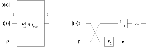
Figure 3: The general circuit scheme for implementing the cyclic POVM (left side) and the circuit for implementing the cyclic POVM for $m=4$ (right side).

The Fourier transform can be implemented efficiently if $m$ is a power of two [7]. Furthermore, the embedding into a qubit register is straightforward since we do not need zero operators in this case. In summary, the cyclic POVM can be implemented efficiently on a qubit register if $m$ is a power of two. For instance, the quantum circuit for the implementation of the cyclic POVM is shown in Figure 3 for $m=4$. The circuit of $F_{4}^{\dagger}$ is the standard circuit for Fourier transforms [7]. Note that the first permutation of the qubits can be removed when we change the order of the input.

5 Dihedral groups

The cyclic symmetry group of an $m$-sided regular polygon which we considered in the previous section is a subgroup of the dihedral group. The dihedral group consists of all rotations which map the $m$-sided regular polygon onto itself. In contrast to the cyclic group we allow the rotations to have different axes. For a fixed $m\geq 2$, the dihedral group is isomorphic to $D_{m}=\langle r,s\rangle$ with $r^{m}=1$, $s^{2}=1$, and $srs=r^{-1}$. In order to use the results for the cyclic groups, we consider the same orientation of the regular polygon as in the previous section, i.e., the face of the polygon is orthogonal to the $z$-axis. Furthermore, we assume that at least one vertex is an element of the $x$-axis. Due to this orientation, the element $r$ corresponds to the $2\pi/m$ rotation about the $z$-axis and the element $s$ corresponds to the $\pi$ rotation about the $x$-axis. In the Hilbert space these rotations correspond to the matrices

$$\left(\begin{array}[]{cc}1&0\\ 0&\omega\end{array}\right)\;{\rm and}\;\;\left(\begin{array}[]{cc}0&1\\ 1&0\end{array}\right)$$

where $\omega:={\rm exp}(-2\pi i/m)$ is a $m$th complex root of unity. We can define a projective representation of the group $D_{m}$ by mapping the element $r\in D_{m}$ to the first matrix and the element $s\in D_{m}$ to the second matrix.

We consider the orbit of a vector under the action of the dihedral group $D_{m}$. Let $(\alpha,\beta)^{T}\in{\mathbb{C}}^{2}$ with $|\alpha|^{2}+|\beta|^{2}=1$. Since a global phase factor of a vector is physically irrelevant we assume $\alpha\in{\mathbb{R}}$ without loss of generality. Under the action of the dihedral group the orbit contains the vectors $(\alpha,\beta\omega^{j})^{T}$ and $(\beta,\alpha\omega^{j})^{T}$ with $j\in\{0,\ldots,m-1\}$. An example of the orbit is shown in Figure 4.

Figure 4: Points of the dihedral POVM with $m=5$.

We have at most $n=2m$ vectors. In the following, we assume that the orbit contains $2m$ elements. If the orbit of $D_{m}$ contains less than $2m$ points we have either the case that all points are on the $xy$-plane (and the POVM consists of a single orbit under the group $C_{m}$) or we have only the two points $(1,0)^{T}$ and $(0,1)^{T}$ defining an orthogonal measurement. Since

$$\sum_{j}\left(\begin{array}[]{c}\alpha\\ \beta\omega^{j}\end{array}\right)(\alpha,{\overline{\beta}}\omega^{-j})+\sum_{j}\left(\begin{array}[]{c}\beta\\ \alpha\omega^{j}\end{array}\right)({\overline{\beta}},\alpha\omega^{-j})=mI_{2},$$

we rescale $\alpha$ and $\beta$ with the factor $\sqrt{1/m}$ to obtain a POVM.

We now consider the implementation of the dihedral POVM. In order to analyze the structure, we do not consider the embedding of the constructed system into a qubit register in the first place. The orbit under the action of $D_{m}$ breaks into two orbits under the action of the subgroup $C_{m}$. The two orbits can be obtained by the action of $C_{m}$ on the vectors $(\alpha,\beta)^{T}$ and $(\beta,\alpha)^{T}$. Therefore, we expect to obtain implementations of the dihedral POVMs which are similar to the implementations in the previous section. With an appropriate order of the vectors we have the matrix

$$M=\left(\begin{array}[]{cccc|cccc}\alpha&\alpha&\ldots&\alpha&\beta&\beta&\ldots&\beta\\ \beta&\beta\omega&\ldots&\beta\omega^{m-1}&\alpha&\alpha\omega&\ldots&\alpha\omega^{m-1}\end{array}\right)\in{\mathbb{C}}^{2\times 2m}.$$

For even $m$, this matrix can be extended to the unitary matrix

$${\tilde{M}}=Q\left(\begin{array}[]{cccc|cccc}\alpha&\alpha&\ldots&\alpha&\beta&\beta&\ldots&\beta\\ \alpha&\alpha\omega&\ldots&\alpha\omega^{m-1}&-{\overline{\beta}}&-{\overline{\beta}}\omega&\ldots&-{\overline{\beta}}\omega^{m-1}\\ \alpha&\alpha\omega^{2}&\ldots&\alpha\omega^{2(m-1)}&\beta&\beta\omega^{2}&\ldots&\beta\omega^{2(m-1)}\\ \vdots&&&\vdots&\vdots&&&\vdots\\ \alpha&\alpha\omega^{m-1}&\ldots&\alpha\omega^{(m-1)(m-1)}&-{\overline{\beta}}&-{\overline{\beta}}\omega^{m-1}&\ldots&-{\overline{\beta}}\omega^{(m-1)(m-1)}\\ \hline\cr&&&&&&\\[-9.95863pt] {\overline{\beta}}&{\overline{\beta}}&\ldots&{\overline{\beta}}&-\alpha&-\alpha&\ldots&-\alpha\\ \beta&\beta\omega&\ldots&\beta\omega^{m-1}&\alpha&\alpha\omega&\ldots&\alpha\omega^{m-1}\\ {\overline{\beta}}&{\overline{\beta}}\omega^{2}&\ldots&{\overline{\beta}}\omega^{2(m-1)}&-\alpha&-\alpha\omega^{2}&\ldots&-\alpha\omega^{2(m-1)}\\ \vdots&&&\vdots&\vdots&&&\vdots\\ \beta&\beta\omega^{m-1}&\ldots&\beta\omega^{(m-1)(m-1)}&\alpha&\alpha\omega^{m-1}&\ldots&\alpha\omega^{(m-1)(m-1)}\end{array}\right)$$

with a permutation matrix $Q\in{\mathbb{C}}^{n\times n}$ fixing the first row and mapping the $(m+2)$nd row to the second row. For odd $m$, the extended matrix is similar. We only have to write $\beta\omega^{(m-1)j}$ instead of $-{\overline{\beta}}\omega^{(m-1)j}$ in the $m$th row. In the last row we write ${\overline{\beta}}\omega^{(m-1)j}$ and $-\alpha\omega^{(m-1)j}$ instead of $\beta\omega^{(m-1)j}$ and $\alpha\omega^{(m-1)j}$, respectively. In order to simplify notation, we mainly consider the case of even $m$ in the following. The constructions for odd $m$ are similar.

We consider a decomposition of the matrix $Q^{\dagger}{\tilde{M}}$ to obtain a decomposition of ${\tilde{M}}$. The matrix $Q^{\dagger}{\tilde{M}}$ can be multiplied with $I_{2}\otimes F_{m}^{\dagger}$ from the right leading to

$$T=\sqrt{m}\left(\begin{array}[]{ll}{\rm diag}(\alpha,\alpha,\alpha,\ldots,\alpha,\alpha)&{\rm diag}(+\beta,-{\overline{\beta}},+\beta,\ldots,+\beta,-{\overline{\beta}})\\ {\rm diag}({\overline{\beta}},\beta,{\overline{\beta}},\ldots,{\overline{\beta}},\beta)&{\rm diag}(-\alpha,+\alpha,-\alpha,\ldots,-\alpha,+\alpha)\end{array}\right).$$

We now embed the system with $n=2m$ dimensions into a qubit register. We consider a register with $l$ qubits where $r:=2^{l}\geq n$. We replace the matrix $T$ with the matrix $T_{r}$ of the same structure but of size $r$. This is done by extending each of the four diagonal components to a diagonal matrix in ${\mathbb{C}}^{(r/2)\times(r/2)}$ while conserving the structure. For instance, the matrix

$$T=\sqrt{3}\left(\begin{array}[]{ccc|ccc}\alpha&&&\beta\\ &\alpha&&&-{\overline{\beta}}\\ &&\alpha&&&\beta\\ \hline\cr&&&&\\[-9.95863pt] {\overline{\beta}}&&&-\alpha\\ &\beta&&&\alpha\\ &&{\overline{\beta}}&&&-\alpha\end{array}\right)$$

is extended to the matrix

$$T_{8}=\sqrt{3}\left(\begin{array}[]{cccc|cccc}\alpha&&&&\beta\\ &\alpha&&&&-{\overline{\beta}}\\ &&\alpha&&&&\beta\\ &&&\alpha&&&&-{\overline{\beta}}\\ \hline\cr&&&&\\[-9.95863pt] {\overline{\beta}}&&&&-\alpha\\ &\beta&&&&\alpha\\ &&{\overline{\beta}}&&&&-\alpha\\ &&&\beta&&&&\alpha\end{array}\right).$$

Furthermore, in the factorization $T=Q^{\dagger}{\tilde{M}}(I_{2}\otimes F_{m}^{\dagger})$ the matrix $Q$ is replaced by a permutation matrix $Q_{r}\in{\mathbb{C}}^{r\times r}$ that fixes the first row and maps the $(r/2+2)$nd row to the second row. In qubit notation, this permutation matrix can be described by $|0\ldots 0\rangle\mapsto|0\ldots 0\rangle$ and $|10\ldots 01\rangle\mapsto|00\ldots 01\rangle$. This permutation can be implemented by an XOR-gate on the first qubit controlled by the last qubit. Other implementations that satisfy the two constraints are also possible. The Fourier transform $F_{m}$ is replaced by $F_{m}\oplus I_{r/2-m}$. In summary, we obtain a matrix ${\tilde{M}}_{r}$ that is defined by the equation

$${\tilde{M}}_{r}=Q_{r}T_{r}(I_{2}\otimes(F_{m}\oplus I_{r/2-m}))\in{\mathbb{C}}^{r\times r}.$$ (1)

This matrix is a unitary extension of the matrix $M$ corresponding to the dihedral POVM with some zero operators as discussed in Section 2. Our example with $T_{8}$ leads to the matrix

$$Q_{8}^{\dagger}{\tilde{M}}_{8}=\left(\begin{array}[]{cccc|cccc}\alpha&\alpha&\alpha&0&\beta&\beta&\beta&0\\ \alpha&\alpha\omega&\alpha\omega^{2}&0&-{\overline{\beta}}&-{\overline{\beta}}\omega&-{\overline{\beta}}\omega^{2}&0\\ \alpha&\alpha\omega^{2}&\alpha\omega&0&\beta&\beta\omega^{2}&\beta\omega&0\\ 0&0&0&\sqrt{3}\alpha&0&0&0&-\sqrt{3}\,{\overline{\beta}}\\ \hline\cr&&&&\\[-9.95863pt] {\overline{\beta}}&{\overline{\beta}}&{\overline{\beta}}&0&-\alpha&-\alpha&-\alpha&0\\ \beta&\beta\omega&\beta\omega^{2}&0&\alpha&\alpha\omega&\alpha\omega^{2}&0\\ {\overline{\beta}}&{\overline{\beta}}\omega^{2}&{\overline{\beta}}\omega&0&-\alpha&-\alpha\omega^{2}&-\alpha\omega&0\\ 0&0&0&\sqrt{3}\beta&0&0&0&\sqrt{3}\alpha\end{array}\right).$$

The matrix $Q_{8}$ maps the sixth row to the second row leading to the first two rows

$$\left(\begin{array}[]{cccc|cccc}\alpha&\alpha&\alpha&0&\beta&\beta&\beta&0\\ \beta&\beta\omega&\beta\omega^{2}&0&\alpha&\alpha\omega&\alpha\omega^{2}&0\end{array}\right)$$

with two zero columns that do not change the POVM due to zero probability. For convenience, we shift the qubits according to the mapping $|x_{1}\ldots x_{l-1}x_{l}\rangle\mapsto|x_{l}x_{1}\ldots x_{l-1}\rangle$. We denote this permutation by $R$. After this reordering of qubits the matrix $T_{r}$ takes the simple form

$$RT_{r}R^{\dagger}=A\otimes I_{r/4}:=\sqrt{m}\left(\begin{array}[]{cccc}\alpha&\beta&0&0\\ {\overline{\beta}}&-\alpha&0&0\\ 0&0&\alpha&-{\overline{\beta}}\\ 0&0&\beta&\alpha\end{array}\right)\otimes I_{r/4}.$$

By combining this equation with Equation (1) we get the factorization

$${\tilde{M}}^{\dagger}_{r}=(I_{2}\otimes(F_{m}^{\dagger}\oplus I_{r/2-m}))R^{\dagger}(A^{\dagger}\otimes I_{r/4})RQ_{r}^{\dagger}.$$

Translating this equation into a quantum circuit, the decomposition of ${\tilde{M}}_{r}$ leads to the circuit scheme shown in Figure 5.

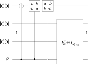
Figure 5: A quantum circuit for implementing the dihedral POVM. We set $a:=\sqrt{m}\alpha$ and $b:=\sqrt{m}\beta$ to simplify notation.

The operation $A^{\dagger}$ is decomposed as

$$A^{\dagger}=\sqrt{m}\left(\begin{array}[]{cccc}\alpha&\beta&0&0\\ {\overline{\beta}}&-\alpha&0&0\\ 0&0&\sqrt{1/m}&0\\ 0&0&0&\sqrt{1/m}\end{array}\right)\sqrt{m}\left(\begin{array}[]{cccc}\sqrt{1/m}&0&0&0\\ 0&\sqrt{1/m}&0&0\\ 0&0&\alpha&{\overline{\beta}}\\ 0&0&-\beta&\alpha\end{array}\right)$$

corresponding to the second and third gates from the left in Figure 5. We do not have to implement the permutation $R$ explicitly if the controlled one-qubit operations are applied to appropriate qubit pairs. The given circuit can be slightly simplified by merging the first two gates from the left to a single controlled gate with the operation

$$\sqrt{m}\left(\begin{array}[]{cc}\alpha&{\overline{\beta}}\\ -\beta&\alpha\end{array}\right)\left(\begin{array}[]{cc}0&1\\ 1&0\end{array}\right)=\sqrt{m}\left(\begin{array}[]{cc}{\overline{\beta}}&\alpha\\ \alpha&-\beta\end{array}\right).$$

As discussed in the previous section the Fourier transform $F_{m}$ can be implemented with a polylogarithmical number of gates if $m$ is a power of two. Consequently, the dihedral POVM can be implemented efficiently in these cases.

6 Tetrahedron

The tetrahedron is the platonic solid with four faces. The symmetry group of the tetrahedron is isomorphic to the alternating group $A_{4}$. This group consists of the twelve permutations of four elements with positive signum. We consider the POVM corresponding to the vertices of the tetrahedron in the Bloch sphere. The tetrahedron is shown Figure 6.

Figure 6: The tetrahedron with two edges perpendicular to the $z$-axis.

For instance, the vertex $1$ is given by the vector $(\sqrt{2/3},0,\sqrt{1/3})^{T}\in{\mathbb{R}}^{3}$. The vertices of the tetrahedron correspond to the vectors

$$\left(\begin{array}[]{c}\alpha\\ \beta\end{array}\right),\left(\begin{array}[]{c}\alpha\\ -\beta\end{array}\right),\left(\begin{array}[]{c}\beta\\ \alpha i\end{array}\right),\left(\begin{array}[]{c}\beta\\ -\alpha i\end{array}\right)\in{\mathbb{C}}^{2}$$ (2)

with $\alpha=\sqrt{(3+\sqrt{3})/6}$ and $\beta=\sqrt{(3-\sqrt{3})/6}$. The first pair of vectors corresponds to the vertices $1$ and $2$, the second pair corresponds to the vertices $3$ and $4$. Note the similarity of these vectors to the vectors

$$\left(\begin{array}[]{c}\alpha\\ \beta\end{array}\right),\left(\begin{array}[]{c}\alpha\\ -\beta\end{array}\right),\left(\begin{array}[]{c}\beta\\ \alpha\end{array}\right),\left(\begin{array}[]{c}\beta\\ -\alpha\end{array}\right).$$

These vectors result from the action of the dihedral group with $m=2$ as considered in previous section with the vector $(\alpha,\beta)^{T}$. The factor $i$ in the second component of the last two vectors of Line (2) results from the $\pi/2$ rotation about the $z$-axis of the lower edge with vertices 3 and 4 relative to the upper edge with vertices 1 and 2. This rotation corresponds to the matrix ${\rm diag}(1,i)\in{\mathbb{C}}^{2\times 2}$. Due to the equation

$$\left(\begin{array}[]{c}\alpha\\ \beta\end{array}\right)(\alpha,\beta)+\left(\begin{array}[]{c}\alpha\\ -\beta\end{array}\right)(\alpha,-\beta)+\left(\begin{array}[]{c}\beta\\ \alpha i\end{array}\right)(\beta,-\alpha i)+\left(\begin{array}[]{c}\beta\\ -\alpha i\end{array}\right)(\beta,\alpha i)=2I_{2}$$

we have the matrix

$$M=\left(\begin{array}[]{cc|cc}\alpha&\alpha&\beta&\beta\\ \beta&-\beta&\alpha i&-\alpha i\end{array}\right)\in{\mathbb{C}}^{2\times 4}$$

with the rescaled elements $\alpha=\sqrt{(3+\sqrt{3})/12}$ and $\beta=\sqrt{(3-\sqrt{3})/12}$. This matrix can be extended to the unitary matrix

$${\tilde{M}}=Q\left(\begin{array}[]{cc|cc}\alpha&\alpha&\beta&\beta\\ \alpha&-\alpha&-\beta\,i&\beta\,i\\ \hline\cr\beta&\beta&-\alpha&-\alpha\\ \beta&-\beta&\alpha\,i&-\alpha\,i\end{array}\right)\in{\mathbb{C}}^{4\times 4}$$

acting on a register of two qubits with the permutation matrix

$$Q=\left(\begin{array}[]{cccc}1&0&0&0\\ 0&0&0&1\\ 0&0&1&0\\ 0&1&0&0\end{array}\right)\in{\mathbb{C}}^{4\times 4}.$$

The matrix $Q$ can be implemented by an XOR-gate on the first qubit controlled by the second qubit. We consider the decomposition of $Q^{\dagger}{\tilde{M}}$ to obtain a decomposition of ${\tilde{M}}$. After multiplying $Q^{\dagger}{\tilde{M}}$ with $(I_{2}\otimes F_{2})\in{\mathbb{C}}^{4\times 4}$ we have

$$Q^{\dagger}{\tilde{M}}(I_{2}\otimes F_{2})=\sqrt{2}\left(\begin{array}[]{cc|cc}\alpha&0&\beta&0\\ 0&\alpha&0&-\beta\,i\\ \hline\cr\beta&0&-\alpha&0\\ 0&\beta&0&\alpha\,i\end{array}\right)\in{\mathbb{C}}^{4\times 4}$$

and after multiplying this matrix with ${\rm diag}(1,1,1,i)\in{\mathbb{C}}^{4\times 4}$

Figure 7: The circuit for the tetrahedral POVM. We set $a:=\sqrt{2}\alpha$ and $b:=\sqrt{2}\beta$ to simplify notation.

from the right we have the equation

$$Q^{\dagger}{\tilde{M}}(I_{2}\otimes F_{2})\left(\begin{array}[]{cccc}1&0&0&0\\ 0&1&0&0\\ 0&0&1&0\\ 0&0&0&i\end{array}\right)=\left(\sqrt{2}\left(\begin{array}[]{cc}\alpha&\beta\\ \beta&-\alpha\end{array}\right)\otimes I_{2}\right)\in{\mathbb{C}}^{4\times 4}.$$ (3)

The matrix ${\rm diag}(1,1,1,i)$ corresponds to a controlled phase gate ${\rm diag}(1,i)$ on the second qubit. Using Equation (3) we get the equation

$${\tilde{M}}^{\dagger}=(I_{2}\otimes F_{2})\left(\begin{array}[]{cccc}1&0&0&0\\ 0&1&0&0\\ 0&0&1&0\\ 0&0&0&i\end{array}\right)\left(\sqrt{2}\left(\begin{array}[]{cc}\alpha&\beta\\ \beta&-\alpha\end{array}\right)\otimes I_{2}\right)Q^{\dagger}.$$

Consequently, the circuit in Figure 7 implements the transformation ${\tilde{M}}^{\dagger}$ for the POVM corresponding to the tetrahedron.

7 Cube

The POVM associated with a cube in the Bloch sphere is a special case of the dihedral POVMs considered in Section 5 with $m=4$. Nevertheless, we consider the implementation of the cubic POVM in this section since we can obtain a smaller circuit by using the special values of $\alpha$ and $\beta$. As in Section 5 we rotate the cube in the Bloch sphere to obtain a face perpendicular to the $z$-axis. Furthermore, we can rotate the cube about this axis to get points corresponding to the vectors

$$\left(\begin{array}[]{c}\alpha\\ \beta\end{array}\right),\left(\begin{array}[]{c}\alpha\\ \beta i\end{array}\right),\left(\begin{array}[]{c}\alpha\\ -\beta\end{array}\right),\left(\begin{array}[]{c}\alpha\\ -\beta i\end{array}\right),\left(\begin{array}[]{c}\beta\\ -\alpha\end{array}\right),\left(\begin{array}[]{c}\beta\\ -\alpha i\end{array}\right),\left(\begin{array}[]{c}\beta\\ \alpha\end{array}\right),\left(\begin{array}[]{c}\beta\\ \alpha i\end{array}\right)\in{\mathbb{C}}^{2}$$

with $\alpha=\sqrt{(3+\sqrt{3})/6}$ and $\beta=\sqrt{(3-\sqrt{3})/6}$. The first four vectors correspond to vertices 1–4 in Figure 8 and

Figure 8: The cube with two faces perpendicular to the $z$-axis.

the last four vectors correspond to vertices 5–8. For instance, the vertex $1$ corresponds to the Bloch point $(\sqrt{2/3},0,\sqrt{1/3})^{T}\in{\mathbb{R}}^{3}$. Note that $\alpha$ and $\beta$ are real numbers. This allows us to use a more efficient construction than in Section 5. Since we have the equation

$$\left(\begin{array}[]{c}\alpha\\ \beta\end{array}\right)(\alpha,\beta)+\ldots+\left(\begin{array}[]{c}\alpha\\ -\beta i\end{array}\right)(\alpha,\beta i)+\left(\begin{array}[]{c}\beta\\ -\alpha\end{array}\right)(\beta,-\alpha)+\ldots+\left(\begin{array}[]{c}\beta\\ \alpha i\end{array}\right)(\beta,-\alpha i)=4I_{2}$$

the given vectors define a POVM when we rescale $\alpha$ and $\beta$ with $1/2$. The matrix $M$ corresponding to the POVM is given by

$$M=\left(\begin{array}[]{cccc|cccc}\alpha&\alpha&\alpha&\alpha&\beta&\beta&\beta&\beta\\ \beta&\beta i&-\beta&-\beta i&-\alpha&-\alpha i&\alpha&\alpha i\end{array}\right)\in{\mathbb{C}}^{2\times 8}.$$

In contrast to the construction of the dihedral POVM we use the fact that for even $m$ the element $-1$ is in the set $\{1,\omega,\ldots,\omega^{m-1}\}$ where $\omega:={\rm exp}(-2\pi i/m)$ is an $m$-th complex root of unity. Therefore, we can reorder the vectors $({\overline{\beta}},\alpha\omega^{j})^{T}\in{\mathbb{C}}^{2}$ considered in Section 5 to obtain a matrix $M$ with the partial row $(-\alpha,-\alpha\omega,\ldots,-\alpha\omega^{m-1})$ instead of $(\alpha,\alpha\omega,\ldots,\alpha\omega^{m-1})$. This is besides $\beta\in{\mathbb{R}}$ the second reason that allows a more efficient construction compared to the construction for the dihedral POVM. Using the equation $\beta={\overline{\beta}}$ we can extend $M$ to the unitary matrix

$${\tilde{M}}=Q\left(\begin{array}[]{cccc|cccc}\alpha&\alpha&\alpha&\alpha&\beta&\beta&\beta&\beta\\ \alpha&\alpha i&-\alpha&-\alpha i&\beta&\beta i&-\beta&-\beta i\\ \alpha&-\alpha&\alpha&-\alpha&\beta&-\beta&\beta&-\beta\\ \alpha&-\alpha i&-\alpha&\alpha i&\beta&-\beta i&-\beta&\beta i\\ \hline\cr\beta&\beta&\beta&\beta&-\alpha&-\alpha&-\alpha&-\alpha\\ \beta&\beta i&-\beta&-\beta i&-\alpha&-\alpha i&\alpha&\alpha i\\ \beta&-\beta&\beta&-\beta&-\alpha&\alpha&-\alpha&\alpha\\ \beta&-\beta i&-\beta&\beta i&-\alpha&\alpha i&\alpha&-\alpha i\end{array}\right)$$

acting on a register of three qubits with a permutation $Q$ satisfying $|000\rangle\mapsto|000\rangle$ and $|101\rangle\mapsto|001\rangle$ in qubit notation. For instance, the permutation can be implemented by a single XOR-gate on the first qubit controlled by the third. We now consider the special structure of $Q^{\dagger}{\tilde{M}}$ to obtain a decomposition of ${\tilde{M}}^{\dagger}$. More precisely, the matrix $Q^{\dagger}{\tilde{M}}$ can be written as the following tensor product

$$Q^{\dagger}{\tilde{M}}=\left(2\left(\begin{array}[]{cc}\alpha&\beta\\ \beta&-\alpha\end{array}\right)\otimes F_{4}\right)\in{\mathbb{C}}^{8\times 8}.$$

This leads to the identity

$${\tilde{M}}^{\dagger}=\left(2\left(\begin{array}[]{cc}\alpha&\beta\\ \beta&-\alpha\end{array}\right)\otimes F_{4}^{\dagger}\right)Q^{\dagger}\in{\mathbb{C}}^{8\times 8}$$

defining the quantum circuit given in Figure 9.

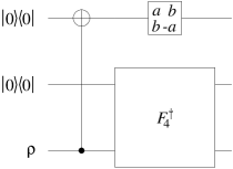
Figure 9: The circuit implementing the cubic POVM. We set $a:=2\alpha$ and $b:=2\beta$ to simplify notation.

Compared to the general circuit in Section 5 we are able to replace two controlled gates by a single uncontrolled gate.

8 Octahedron

The symmetry group of the octahedron is identical to the symmetry group of the cube since the octahedron is the dual polyhedron of the cube. The group is isomorphic to the symmetric group $S_{4}$. This group consists of all $24$ permutations of four elements. A simple implementation of the octahedral POVM can be obtained by the orientation of the octahedron as shown in Figure 10 where the upper face with vertices 1–3 and the lower face with vertices 4–6 are perpendicular to the $z$-axis. Vertex $1$ corresponds to the real vector $(\sqrt{2/3},0,\sqrt{1/3})^{T}\in{\mathbb{R}}^{3}$. The complex vectors corresponding to the points 1–6 are given by

Figure 10: The octahedron with two faces perpendicular to the $z$-axis.

$$\left(\begin{array}[]{c}\alpha\\ \beta\end{array}\right),\left(\begin{array}[]{c}\alpha\\ \beta\omega\end{array}\right),\left(\begin{array}[]{c}\alpha\\ \beta\omega^{2}\end{array}\right),\left(\begin{array}[]{c}\beta\\ -\alpha\end{array}\right),\left(\begin{array}[]{c}\beta\\ -\alpha\omega\end{array}\right),\left(\begin{array}[]{c}\beta\\ -\alpha\omega^{2}\end{array}\right)\in{\mathbb{C}}^{2}$$

where $\omega:={\rm exp}(-2\pi i/3)$ is a root of unity, $\alpha=\sqrt{(3+\sqrt{3})/6}$ and $\beta=\sqrt{(3-\sqrt{3})/6}$. The first three vectors correspond to the upper three vertices 1–3 of the octahedron, the last three vectors to the lower three vertices 4–6. Despite the negative sign of the second component of the last three elements, these vectors are identical with the vectors

$$\left(\begin{array}[]{c}\alpha\\ \beta\end{array}\right),\left(\begin{array}[]{c}\alpha\\ \beta\omega\end{array}\right),\left(\begin{array}[]{c}\alpha\\ \beta\omega^{2}\end{array}\right),\left(\begin{array}[]{c}\beta\\ \alpha\end{array}\right),\left(\begin{array}[]{c}\beta\\ \alpha\omega\end{array}\right),\left(\begin{array}[]{c}\beta\\ \alpha\omega^{2}\end{array}\right)\in{\mathbb{C}}^{2}.$$

The latter vectors are obtained by the vector $(\alpha,\beta)^{T}$ under the action of the dihedral group $D_{3}$ as discussed in Section 5. Similar to the factor $i$ in two vectors of the tetrahedral POVM in Section 6, the negative sign results from the $\pi$ rotation about the $z$-axis of the lower three vertices 4–6 relative to the upper three vertices 1–3. Since

$$\left(\begin{array}[]{c}\alpha\\ \beta\end{array}\right)(\alpha,\beta)+\ldots+\left(\begin{array}[]{c}\beta\\ -\alpha\omega^{2}\end{array}\right)(\beta,-\alpha\omega)=3I_{2}$$

we rescale $\alpha$ and $\beta$ with the factor $\sqrt{1/3}$ to obtain a POVM. Therefore, we have

$$M=\left(\begin{array}[]{ccc|ccc}\alpha&\alpha&\alpha&\beta&\beta&\beta\\ \beta&\beta\omega&\beta\omega^{2}&-\alpha&-\alpha\omega&-\alpha\omega^{2}\end{array}\right)\in{\mathbb{C}}^{2\times 6}.$$ (4)

As already discussed, we have the negative signs in Equation (4) because the lower face is rotated relatively to the upper face. This is different from the cubic POVM where we have to reorder the operators (compared to the dihedral case) in order to get the negative signs in the second component of the last four vectors. To see this, we write these components as $-\alpha$, $-\alpha\omega$, $-\alpha\omega^{2}$ and $-\alpha\omega^{3}$ with $\omega=i$ as in the dihedral case.

We now consider the extension of $M$ to a unitary matrix ${\tilde{M}}$. As in Section 5 we do not embed the system with six dimensions into a qubit register in the first place. The matrix $M$ corresponds to the first two rows of the matrix

$${\tilde{M}}=Q\left(\begin{array}[]{ccc|ccc}\alpha&\alpha&\alpha&\beta&\beta&\beta\\ \alpha&\alpha\omega&\alpha\omega^{2}&\beta&\beta\omega&\beta\omega^{2}\\ \alpha&\alpha\omega^{2}&\alpha\omega&\beta&\beta\omega^{2}&\beta\omega\\ \hline\cr\beta&\beta&\beta&-\alpha&-\alpha&-\alpha\\ \beta&\beta\omega&\beta\omega^{2}&-\alpha&-\alpha\omega&-\alpha\omega^{2}\\ \beta&\beta\omega^{2}&\beta\omega&-\alpha&-\alpha\omega^{2}&-\alpha\omega\end{array}\right)$$

where $Q$ is a permutation matrix that fixes the first row and maps the fifth row to the second. Similar to the previous section, this matrix can be written as

$${\tilde{M}}=Q\left(\sqrt{3}\left(\begin{array}[]{cc}\alpha&\beta\\ \beta&-\alpha\end{array}\right)\otimes F_{3}\right)\in{\mathbb{C}}^{6\times 6}.$$ (5)

We now translate the decomposition of ${\tilde{M}}$ into a circuit. We have to embed the system with six dimensions into a qubit register with at least three qubits. This can be done by replacing the Fourier matrix $F_{3}$ in Equation (5) with $F_{3}\oplus I_{1}$ where $I_{1}\in{\mathbb{C}}^{1\times 1}$ denotes the identity matrix of size one. This replacement leads to the matrix

$${\tilde{M}}_{8}=Q_{8}\left(\begin{array}[]{cccc|cccc}\alpha&\alpha&\alpha&0&\beta&\beta&\beta&0\\ \alpha&\alpha\omega&\alpha\omega^{2}&0&\beta&\beta\omega&\beta\omega^{2}&0\\ \alpha&\alpha\omega^{2}&\alpha\omega&0&\beta&\beta\omega^{2}&\beta\omega&0\\ 0&0&0&\sqrt{3}\alpha&0&0&0&\sqrt{3}\beta\\ \hline\cr\beta&\beta&\beta&0&-\alpha&-\alpha&-\alpha&0\\ \beta&\beta\omega&\beta\omega^{2}&0&-\alpha&-\alpha\omega&-\alpha\omega^{2}&0\\ \beta&\beta\omega^{2}&\beta\omega&0&-\alpha&-\alpha\omega^{2}&-\alpha\omega&0\\ 0&0&0&\sqrt{3}\beta&0&0&0&-\sqrt{3}\alpha\end{array}\right)$$

where $Q_{8}\in{\mathbb{C}}^{8\times 8}$ is a permutation matrix that fixes the first row and maps the sixth

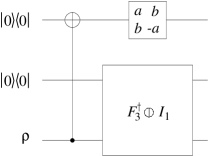
Figure 11: A circuit for implementing the octahedral POVM. We set $a:=\sqrt{3}\alpha$ and $b:=\sqrt{3}\beta$ to simplify notation.

row to the second row. In qubit notation, these constraints are given by $|000\rangle\mapsto|000\rangle$ and $|101\rangle\mapsto|001\rangle$. For instance, this transformation can be implemented by an XOR-gate on the first qubit controlled by the last qubit. If we restrict ${\tilde{M}}_{8}$ to the first two rows we get the matrix

$$\left(\begin{array}[]{cccc|cccc}\alpha&\alpha&\alpha&0&\beta&\beta&\beta&0\\ \beta&\beta\omega&\beta\omega^{2}&0&-\alpha&-\alpha\omega&-\alpha\omega^{2}&0\end{array}\right)$$

corresponding to the desired POVM. The POVM operator corresponding to the fourth and eighth column is $0_{2}\in{\mathbb{C}}^{2\times 2}$ leading to a zero probability for all states $\rho\in{\mathbb{C}}^{2\times 2}$. In summary, we have the equation

$${\tilde{M}}_{8}^{\dagger}=\left(\sqrt{3}\left(\begin{array}[]{cc}\alpha&\beta\\ \beta&-\alpha\end{array}\right)\otimes\left(F_{3}^{\dagger}\oplus I_{1}\right)\right)Q_{8}^{\dagger}$$

for the implementation of the octahedral POVM. This equation corresponds to the circuit shown in Figure 11.

9 Dodecahedron

The dodecahedron is the platonic solid with twelve faces and twenty vertices. The symmetry group of the dodecahedron is isomorphic to the alternating group $A_{5}$. This group contains the sixty permutations of five elements with positive signum. The dodecahedron is shown in Figure 12. The upper face with vertices 1–5 and the lower face with vertices 6–10 are perpendicular to the $z$-axis. The point

$$\left(\sqrt{\frac{10-2\sqrt{5}}{15}}\,,\;0\,,\;\sqrt{\frac{5+2\sqrt{5}}{15}}\right)^{T}\in{\mathbb{R}}^{3}$$

corresponds to vertex $1$. This orientation of the dodecahedron in the Bloch sphere leads to a simple construction of the dodecahedral POVM. With $\omega:={\rm exp}(-2\pi i/5)$, the points on the Bloch sphere correspond to the complex vectors

Figure 12: The dodecahedron with two faces perpendicular to the $z$-axis.

$$\left(\begin{array}[]{c}\alpha\\ \beta\omega^{j}\end{array}\right),\left(\begin{array}[]{c}\beta\\ -\alpha\omega^{j}\end{array}\right),\left(\begin{array}[]{c}\gamma\\ \delta\omega^{j}\end{array}\right),\left(\begin{array}[]{c}\delta\\ -\gamma\omega^{j}\end{array}\right)\in{\mathbb{C}}^{2}$$ (6)

where $j\in\{0,\ldots,4\}$. The vectors $(\alpha,\beta\omega^{j})^{T}$ correspond to the points 1–5, the vectors $(\beta,-\alpha\omega^{j})^{T}$ to 6–10, the vectors $(\gamma,\delta\omega^{j})^{T}$ to 11–15, and the vectors $(\delta,\gamma\omega^{j})^{T}$ to the points 16–20. The parameters $\alpha,\beta,\gamma,$ and $\delta$ are defined as follows:

$$\alpha=\sqrt{\frac{1}{2}+\frac{1}{30}\sqrt{75+30\sqrt{5}}}\,,\;\beta=\sqrt{\frac{1}{2}-\frac{1}{30}\sqrt{75+30\sqrt{5}}}$$

and

$$\gamma=\sqrt{\frac{1}{2}+\frac{1}{30}\sqrt{75-30\sqrt{5}}}\,,\;\delta=\sqrt{\frac{1}{2}-\frac{1}{30}\sqrt{75-30\sqrt{5}}}.$$

Due to the equation

$$\left(\begin{array}[]{c}\alpha\\ \beta\end{array}\right)(\alpha,\beta)+\ldots+\left(\begin{array}[]{c}\delta\\ \gamma\omega^{4}\end{array}\right)(\delta,\gamma\omega^{-4})=10I_{2}$$

we rescale the elements $\alpha,\beta,\gamma,\delta$ with the factor $\sqrt{1/10}$ to obtain a POVM. In contrast to the constructions of Sections 5–8 the points on the Bloch sphere decompose into four different orbits under the rotation about the $z$-axis. Note that there are two pairs of orbits. In Line (6) the vectors $(\alpha,\beta\omega^{j})^{T}$ and $(\beta,-\alpha\omega^{j})^{T}$ are similar to the vectors $(\alpha,\beta\omega^{j})^{T}$ and $(\beta,\alpha\omega^{j})^{T}$. The latter vectors are the orbit of $(\alpha,\beta)^{T}$ under the dihedral group with $m=5$ as considered in Section 5. As in the previous section a $\pi$ rotation of one orbit relative to the other orbit causes the negative sign of the elements $(\beta,-\alpha\omega^{j})^{T}$. Analogously, the second orbit under $D_{5}$ is defined by the third and fourth type of vectors in Line (6). In summary, the vertices of the dodecahedron correspond to two orbits under the dihedral group $D_{5}$ with a $\pi$ rotation about the $z$-axis of some points on each orbit. Consequently, we can expect to use a similar construction as in the previous sections.

We now consider the construction of the circuit for implementing the dodecahedral POVM. For convenience, we do not embed the system into a qubit register in the first place. We have the matrix

$$M=\left(\begin{array}[]{cccc|ccc|ccc|cccc}\alpha&\alpha&\ldots&\alpha&\beta&\ldots&\beta&\gamma&\ldots&\gamma&\delta&\delta&\ldots&\delta\\ \beta&\beta\omega&\ldots&\beta\omega^{4}&-\alpha&\ldots&-\alpha\omega^{4}&\delta&\ldots&\delta\omega^{4}&-\gamma&-\gamma\omega&\ldots&-\gamma\omega^{4}\end{array}\right).$$

This matrix corresponds to the first and second row of the unitary matrix ${\tilde{M}}$ defined by the equation

$${\tilde{M}}=Q\left(A\otimes F_{5}\right)\in{\mathbb{C}}^{20\times 20},$$ (7)

where $Q\in{\mathbb{C}}^{20\times 20}$ is a permutation matrix that fixes the first row and maps the seventh row to the second row. The matrix $A$ is defined by

$$A=\sqrt{5}\left(\begin{array}[]{cccc}\alpha&\beta&\gamma&\delta\\ \beta&-\alpha&\delta&-\gamma\\ \gamma&-\delta&-\alpha&\beta\\ \delta&\gamma&-\beta&-\alpha\end{array}\right).$$

Now, we want to embed the extended system into a register with five qubits. Similar to the construction for the octahedron in Section 8, we can do this by replacing the matrix $F_{5}$ in Equation (7) by the matrix $(F_{5}\oplus I_{3})\in{\mathbb{C}}^{8\times 8}$ where $I_{3}$ denotes the identity matrix of size three. The matrix $Q$ is replaced by a permutation matrix $Q_{32}\in{\mathbb{C}}^{32\times 32}$ that satisfies $|00000\rangle\mapsto|00000\rangle$ and $|01001\rangle\mapsto|00001\rangle$ in the qubit notation. This permutation can be implemented by an XOR-operation on the second qubit controlled by the last qubit. In summary, the matrix ${\tilde{M}}^{\dagger}_{32}$ is defined by the equation

$${\tilde{M}}^{\dagger}_{32}=\left(A^{\dagger}\otimes\left(F_{5}^{\dagger}\oplus I_{3}\right)\right)Q_{32}^{\dagger}.$$

The corresponding circuit is shown in Figure 13.

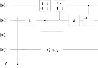
Figure 13: A circuit for implementing the dodecahedral POVM. In order to simplify notation, the elements $\pm 1$ of the gates on the first qubit represent $\pm\sqrt{1/2}$.

Note that the matrix $A^{\dagger}$ can be written as product $A^{\dagger}=\left(I_{2}\oplus(-\sigma_{z})\right)\left(I_{2}\otimes B\right)R\left(I_{2}\otimes C\right)$ with the matrices

$$B=\left(\begin{array}[]{cc}u_{-}&-u_{+}\\ u_{+}&u_{-}\end{array}\right),\;\;C=\left(\begin{array}[]{cc}v_{-}&v_{+}\\ v_{+}&-v_{-}\end{array}\right)$$

and constants

$$u_{\pm}=\sqrt{\frac{1}{2}\pm\sqrt{\frac{3+\sqrt{5}}{24}}}\;,\;\;v_{\pm}=\mp\sqrt{\frac{1}{2}\pm\sqrt{\frac{\sqrt{5}-1}{8\sqrt{5}}}}.$$

The matrix $R$ is the product

$$R=\sqrt{\frac{1}{2}}\left(\begin{array}[]{cccc}1&0&-1&0\\ 0&\sqrt{2}&0&0\\ 1&0&1&0\\ 0&0&0&\sqrt{2}\end{array}\right)\sqrt{\frac{1}{2}}\left(\begin{array}[]{cccc}\sqrt{2}&0&0&0\\ 0&1&0&1\\ 0&0&\sqrt{2}&0\\ 0&-1&0&1\end{array}\right).$$

In Figure 13, the latter two matrices correspond to the two operations on the first qubit which are controlled by the second qubit.

10 Icosahedron

The icosahedron is the dual polyhedron of the dodecahedron. Consequently, the symmetry groups of both platonic solids are identical. We assume the specific orientation of the icosahedron as shown in Figure 14 to obtain a simple construction of the icosahedral POVM. The upper face with vertices 1–3 and the lower face with vertices 4–6 are perpendicular to the $z$-axis. Vertex 1 is given by the vector

$$\left(\sqrt{\frac{10-2\sqrt{5}}{15}}\,,\;0\,,\;\sqrt{\frac{5+2\sqrt{5}}{15}}\right)^{T}\in{\mathbb{R}}^{3}.$$

Figure 14: The icosahedron with two faces perpendicular to the $z$-axis.

The vertices of the icosahedron in the Bloch sphere correspond to the complex vectors

$$\left(\begin{array}[]{c}\alpha\\ \beta\omega^{j}\end{array}\right),\left(\begin{array}[]{c}\beta\\ -\alpha\omega^{j}\end{array}\right),\left(\begin{array}[]{c}\gamma\\ \delta\omega^{j}\end{array}\right),\left(\begin{array}[]{c}\delta\\ -\gamma\omega^{j}\end{array}\right)\in{\mathbb{C}}^{2}$$ (8)

with $j\in\{0,1,2\}$, $\omega:={\rm exp}(-2\pi i/3)$ and

$$\alpha=\sqrt{\frac{1}{2}+\frac{1}{30}\sqrt{75+30\sqrt{5}}}\;\;,\;\;\beta=\sqrt{\frac{1}{2}-\frac{1}{30}\sqrt{75+30\sqrt{5}}}$$

and

$$\gamma=\sqrt{\frac{1}{2}-\frac{1}{30}\sqrt{75-30\sqrt{5}}}\;\;,\;\;\delta=\sqrt{\frac{1}{2}+\frac{1}{30}\sqrt{75-30\sqrt{5}}}.$$

The vectors in Line (8) with $j=0$ correspond to the vertices $1$, $4$, $7$ and $10$ in the given order. As in the case of the dodecahedron we have four orbits under the rotations about the $z$-axis. Therefore, we can expect that a similar construction as in the previous section is possible. Due to the identity

$$\left(\begin{array}[]{c}\alpha\\ \beta\end{array}\right)(\alpha,\beta)+\ldots+\left(\begin{array}[]{c}\delta\\ \gamma\omega^{4}\end{array}\right)(\delta,\gamma\omega^{-4})=6I_{2}$$

we have the matrix

$$M=\left(\begin{array}[]{ccc|ccc|ccc|ccc}\alpha&\alpha&\alpha&\beta&\beta&\beta&\gamma&\gamma&\gamma&\delta&\delta&\delta\\ \beta&\beta\omega&\beta\omega^{2}&-\alpha&-\alpha\omega&-\alpha\omega^{2}&\delta&\delta\omega&\delta\omega^{2}&-\gamma&-\gamma\omega&-\gamma\omega^{2}\end{array}\right),$$

where we rescale $\alpha,\beta,\gamma$ and $\delta$ with the factor $\sqrt{1/6}$. The matrix $M$ consists of the first and second row of the matrix

$${\tilde{M}}=Q\left(A\otimes F_{3}\right)\in{\mathbb{C}}^{12\times 12},$$ (9)

where $Q\in{\mathbb{C}}^{12\times 12}$ is a permutation matrix that fixes the first row and maps the fifth row to the second. Similar to the previous section, the matrix $A$ is given by

$$A=\sqrt{3}\left(\begin{array}[]{cccc}\alpha&\beta&\gamma&\delta\\ \beta&-\alpha&\delta&-\gamma\\ \gamma&-\delta&-\alpha&\beta\\ \delta&\gamma&-\beta&-\alpha\end{array}\right).$$

The embedding into a register with four qubits works analogously to the previous section. We replace $F_{3}$ in Equation (9) by $(F_{3}\oplus I_{1})\in{\mathbb{C}}^{4\times 4}$ where $I_{1}$ denotes the identity matrix of size one. The matrix $Q$ is replaced by the matrix $Q_{16}\in{\mathbb{C}}^{16\times 16}$ that can be described as $|0000\rangle\mapsto|0000\rangle$ and $|0101\rangle\mapsto|0001\rangle$ in the qubit notation. This permutation can be implemented by an XOR-operation on the second qubit controlled by the last qubit. Therefore, Equation (9) translates into

$${\tilde{M}}_{16}^{\dagger}=\left(A^{\dagger}\otimes\left(F_{3}^{\dagger}\oplus I_{1}\right)\right)Q_{16}^{\dagger}.$$

The circuit corresponding to this decomposition of ${\tilde{M}}^{\dagger}_{16}$ is given in Figure 15.

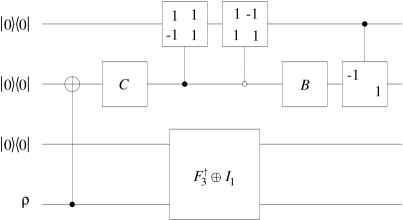
Figure 15: A circuit for implementing the icosahedral POVM. In order to simplify notation, the elements $\pm 1$ of the gates on the first qubit represent $\pm\sqrt{1/2}$.

The matrix $A^{\dagger}$ can be translated into single- and two-qubit gates as shown in the previous section. In this translation we have to replace the constants $u_{\pm}$ and $v_{\pm}$ with

$$u_{\pm}=\frac{1}{10}\sqrt{50\pm 5\sqrt{10(5+\sqrt{5})}}\quad{\rm and}\quad v_{\pm}=\mp\frac{1}{2}\sqrt{2\pm\sqrt{5/3}\mp\sqrt{1/3}}.$$

11 Conclusions

We have shown that all POVMs given by the vertices of platonic solids can be implemented using a discrete Fourier transform and a few other operations. The algorithms use the symmetry of the POVMs. A common feature of all constructions is the partition of the POVM operators into orbits under the action of a cyclic group. Since the Fourier transform allows to implement POVMs associated with an orbit under a cyclic group it is an essential part of all circuits. For most POVMs corresponding to a platonic solid, a tensor product of a Fourier transform and a specific low-dimensional matrix is a central building block of the circuit. The low-dimensional matrix represents in some sense the relations between the orbits.

The implementation of non-symmetric POVMs seems to be a non-trivial task. It would, for instance, be interesting to know which POVMs can be implemented efficiently, i.e., with a number of elementary gates which grows only polynomially in the number $n$ of POVM-operators. For the symmetric POVMs considered in this paper the question of efficiency makes only sense for the cyclic and dihedral POVMs since the size of the other POVMs is fixed. For $n=2^{l}$ the complexity of the Fourier transform $F_{n}$ is only polynomial in $l$. Therefore, the complexity of the circuits for the cyclic and dihedral POVMs grows only polylogarithmically in $n$.

The question of the efficiency of read-out mechanisms for a single bit has no counterpart in classical computer science. Complexity issues in quantum information theory deal not necessarily with the complexity of computational problems. They are also interesting in the context of measurements or state preparation procedures. However, there are some connections between a complexity theory of these non-computational quantum control problems and computational problems [9, 10]. Connections between the complexity of POVM measurements and other complexity issues may be subject of further research.

The authors acknowledge helpful discussions with M. Grassl and M. Rötteler. M. Rötteler brought the problem of implementing symmetric POVMs to our attention. This work was supported by grants of the BMBF project 01/BB01B.

References

[1]E.B. Davies: Quantum theory of open systems,
Academic Press, 1976.
[2]M. Sasaki, S.M. Barnett, R. Jozsa, M. Osaki,
O. Hirota: Accessible information and optimal strategies for real
symmetrical quantum sources, Physical Review A, Vol. 59, No. 5,
pp. 3325–3335, May 1999.
[3]E.B. Davies: Information and Quantum
Measurement, IEEE Transactions on Information Theory, Vol. IT-24,
No. 5, September 1978.
[4]Y.C. Eldar, G.D. Forney: On Quantum Detection and
the Square-Root Measurement, IEEE Transactions on Information Theory,
Vol. 47, pp. 858-872, Mar. 2001.
[5] C. Fuchs: Information Gain vs. State Disturbance
in Quantum Theory, LANL-preprint quant-ph/9611010.
[7]M.A. Nielsen, I.L. Chuang: Quantum Computation
and Quantum Information, Cambridge University Press, 2000.
[8]S. Sternberg: Group theory and physics,
Cambridge University Press, 1994.
[9]D. Janzing, P. Wocjan, Th. Beth: Cooling and
Low Energy State Preparation for 3-local Hamiltonians are
FQMA-complete, LANL-preprint quant-ph/0305050.
[10] P. Wocjan, D. Janzing, Th. Decker, Th. Beth: Measuring 4-local n-qubit observables could probabilistically solve
PSPACE, LANL-preprint quant-ph/0308011.