Structure of multiphoton quantum optics. II. Bipartite systems,
physical processes, and heterodyne squeezed states

Abstract

Extending the scheme developed for a single mode of the electromagnetic field in the preceding paper “Structure of multiphoton quantum optics. I. Canonical formalism and homodyne squeezed states”, we introduce two-mode nonlinear canonical transformations depending on two heterodyne mixing angles. They are defined in terms of hermitian nonlinear functions that realize heterodyne superpositions of conjugate quadratures of bipartite systems. The canonical transformations diagonalize a class of Hamiltonians describing non degenerate and degenerate multiphoton processes. We determine the coherent states associated to the canonical transformations, which generalize the non degenerate two–photon squeezed states. Such heterodyne multiphoton squeezed are defined as the simultaneous eigenstates of the transformed, coupled annihilation operators. They are generated by nonlinear unitary evolutions acting on two-mode squeezed states. They are non Gaussian, highly non classical, entangled states. For a quadratic nonlinearity the heterodyne multiphoton squeezed states define two–mode cubic phase states. The statistical properties of these states can be widely adjusted by tuning the heterodyne mixing angles, the phases of the nonlinear couplings, as well as the strength of the nonlinearity. For quadratic nonlinearity, we study the higher-order contributions to the susceptibility in nonlinear media and we suggest possible experimental realizations of multiphoton conversion processes generating the cubic-phase heterodyne squeezed states.

I Introduction

In this paper we extend to bipartite systems of pairs of correlated modes the multiphoton canonical formalism developed for a single mode of the electromagnetic field in the companion paper ”Structure of multiphoton quantum optics. I. Canonical formalism and homodyne squeezed states” paper1 , which, from now on, we will refer to as Part I. Preliminary to the description of the multiphoton canonical formalism we need to discuss briefly the well established formalism of two-mode quantum optics yuen ; caves . Two–mode non degenerate squeezed states are generated by second order susceptibility contributions excited by laser shots on nonlinear optical media. Due to the second order nonlinearity, the frequency $\Omega$ of a high energy laser splits inside the crystal into a pair of frequencies $\omega_{1},\omega_{2}$ ($\Omega=\omega_{1}+\omega_{2}$) associated to correlated modes of the electromagnetic field (non degenerate down conversion process), with the reversed up conversion process of recomposition of the two frequencies being allowed as well. The degenerate limit $\omega_{1}=\omega_{2}$ can be considered, with the splitted frequencies being associated to a single mode of the electromagnetic field. Two–photon squeezed states are the coherent states of the Hamiltonian which describes the simultaneous creation or annihilation of a photon in each of the correlated modes (or of two photon in a single mode for the degenerate case). The two–photon Hamiltonian is diagonalized by coupled linear canonical transformations. The two–photon squeezed states can be obtained as common eigenstates of the two–mode transformed variables. They can be generated as well by applying a (squeezing) unitary operator on the two-mode vacuum or on the two-mode coherent state; the unitary operator moves the original mode operators to the canonically transformed variables.

When considering possible extensions of the above scheme to multiphoton processes, one natural choice is to consider down–conversion processes in which the carrying laser frequency splits into $n$ frequencies, giving rise to the creation (and later annihilation) of $n$ photons in $n$ correlated modes of the field (or in a single mode of the field in the degenerate limit). However, the related Hamiltonians cannot be exactly diagonalized, and an exact canonical scheme cannot be implemented. In this paper we follow a different route, outlined in Part I for single-mode systems. We consider classes of multiphoton processes in multimode systems such that the number of photons involved in the processes does not correspond in general to the number of excited modes. In such instances, the fully degenerate limit entails that the interaction terms in the Hamiltonians do not in general reduce to simple powers of the creation and annihilation operators. In Part I paper1 , we have introduced degenerate, canonical $n$-photon generalizations of the degenerate, canonical two–photon processes. The single-mode multiphoton generalization has been obtained by using nonlinear operator functions of homodyne superpositions of conjugate quadratures.

To the end of generalizing the canonical formalism to two-mode, non degenerate multiphoton processes, we consider nonlinear operator functions of heterodyne superpositions of the two–mode variables, obtaining coupled two–mode transformed operators with a nonlinear dependence on the original operators. As in the one–mode instance, we show that the canonical conditions reduce to simple algebraic constraints only on the complex coefficients of the transformations, while they are independent of the form of the nonlinear functions.

Upon introducing multiphoton canonical transformations for bipartite systems, we analyze the problems regarding the multiphoton Hamiltonians induced by the transformations, their physical interest, and their experimental realizability. We determine the multiphoton coherent states associated to the transformations, and study their statistical properties. Finally, we show that the two-mode multiphoton coherent states can be generated by acting with a unitary operator on the two–mode vacuum. The structure of the two-mode multiphoton canonical transformations does not allow the realization of the associated coherent states by the displacement operator method, i.e. by the unitary evolution with the interaction Hamiltonian. This problem is similar to that of mapping interacting fields onto free fields in Quantum Field Theory for nonlinear systems. We thus consider the coherent states defined as the simultaneous eigenstates of the coupled canonical transformations. Exploiting the entangled state representation we can then compute their eigenfunctions. The resulting states share important features of the standard coherent states, such as forming an overcomplete basis in Hilbert space. These multiphoton coherent states associated to the nonlinear transformations share squeezing properties as well, and we thus name them (two–mode) heterodyne multiphoton squeezed states (HEMPSS). They are non Gaussian, highly non classical, entangled states. A large part of the present paper is devoted to the characterization and quantification of their physical properties.

The independence of the canonical transformations by the form of the nonlinear functions allows in principle to introduce an infinite number of diagonalizable Hamiltonians. In analogy to the degenerate case we have considered the subclass of Hamiltonians involving only algebraic powers of the heterodyne variables. This choice defines Hamiltonians associated with degenerate and degenerate multiphoton processes in two modes of the electromagnetic field. The higher-order multiphoton processes are related to higher-order contributions to the susceptibility in nonlinear media. We then study in detail only the simplest case of quadratic nonlinearity, which leads to Hamiltonians describing up to four-photon processes. We analyze the photon statistics of the HEMPSS, showing the strong dependence of the interference in phase space by the competing phases entering in the nonlinearity, and by the heterodyne angles. We suggest schemes for a possible experimental realization of the HEMPSS by exploiting contributions to the susceptibility up to the fifth order in nonlinear media. We determine the unitary operator acting on the vacuum to generate the HEMPSS: its form suggests alternative routes to their possible experimental realization.

We remark that multimode nonlinear canonical transformations of the form introduced in the present paper can be defined in principle for generic bosonic systems of atomic, molecular, and condensed matter physics. In such cases however the constraints on the standard form of the kinetic energy term and on the conservation of the total number of particles play a crucial role and must be taken carefully into account. A thorough analysis of the relevance of the nonlinear canonical formalisms for material systems lies thus outside the scope of the present paper.

The paper is organized as follows. In Section II we introduce the two–mode nonlinear canonical transformations and the associated multiphoton Hamiltonians. In Sections III and IV we review the entangled state representation, and exploit it to determine the coherent states of the transformations, defined as the eigenstates of the transformed annihilation operators (heterodyne multiphoton squeezed states, or HEMPSS). In Section V we derive the form of the unitary operators generating the HEMPSS by acting on the two–mode vacuum. In Section VI we study the photon number distribution of the two–mode multiphoton squeezed states. In Section VII we review the theory of quantized fields in nonlinear media, and in Section VIII we present a proposal for a possible experimental generation of the HEMPSS. Finally, in Section IX we draw our conclusions and discuss further future developments.

II Two–mode multiphoton canonical transformations via heterodyne photocurrent variables

In this Section we introduce the two-mode multiphoton canonical formalism. We consider two (correlated) modes of the quantized electromagnetic field. The modes are characterized by the annihilation and creation operators $a_{1}$, $a_{2}$, $a_{1}^{{\dagger}}$ and $a_{2}^{{\dagger}}$, obeying the canonical commutation relations

$$[a_{i},a_{j}^{{\dagger}}]=\delta_{ij}\;,\quad\quad[a_{i},a_{j}]=0\;.$$ (1)

We begin by recalling that the form of the two-mode, linear canonical squeezing transformations is caves :

$$b_{1} = \mu a_{1}+\nu a_{2}^{\dagger}\,,$$

$$b_{2} = \mu a_{2}+\nu a_{1}^{\dagger}\,,$$

with $\mu$, $\nu$ complex numbers. As is well known, the above transformations are canonical if

$$|\mu|^{2}-|\nu|^{2}=1\;,$$ (3)

and the constraint is automatically satisfied by the parametrization

$$\mu=\cosh r\;,\quad\nu=\sinh re^{i\phi}\;,$$ (4)

where $r$ is the squeezing parameter. The transformations Eqs. (LABEL:sst) can be obtained from the original mode operators $a_{1}$, $a_{2}$ by acting with the unitary operator caves

$$S_{12}(\zeta)=\exp(\zeta a_{2}^{\dagger}a_{1}^{\dagger}-{\zeta}^{*}a_{2}a_{1})\,,\,\zeta=re^{i\phi}\,.$$ (5)

The transformed variables $b_{1},b_{2}$ define the diagonalized Hamiltonian

$$H=b_{1}^{{\dagger}}b_{1}+b_{2}^{{\dagger}}b_{2}\,,$$ (6)

which can be written in terms of the fundamental mode operators as:

$$H = (|\mu|^{2}+|\nu|^{2})(a_{1}^{{\dagger}}a_{1}+a_{2}^{{\dagger}}a_{2})+2|\nu|^{2}$$ (7)

$$+ 2\mu^{*}\nu a_{1}^{{\dagger}}a_{2}^{{\dagger}}+2\mu\nu^{*}a_{1}a_{2}\,.$$

The scheme defined by relations Eqs. (LABEL:sst), (4), (5), (7) describes non degenerate two-photon down-conversion processes.

We wish to extend the linear canonical scheme to provide an Hamiltonian description of multiphoton processes. Let us define a new set of transformed variables $b_{1}$ and $b_{2}$ by

$$b_{1} = \mu a_{1}+\nu a_{2}^{\dagger}+\gamma F(a_{1}^{\dagger},a_{2})\;,$$

$$b_{2} = \mu a_{2}+\nu a_{1}^{\dagger}+\chi F^{\dagger}(a_{1}^{\dagger},a_{2})\;.$$

Here $\mu$, $\nu$, $\gamma$ and $\chi$ are complex numbers. The generalization of the two–photon linear canonical transformations is obtained by introducing a nonlinear, operator–valued function $F$ of the creation and annihilation operators. The function $F$ must satisfy some regularity conditions. Even so, the canonical conditions may not in general be satisfied by a completely arbitrary, though well behaved, function. We will now introduce two crucial characterizations of $F$, allowing to select a large class of functions that do satisfy the canonical constraints. First, we assume the argument of $F$ to be of the form

$$\alpha a_{1}^{{\dagger}}+\beta^{*}a_{2}\;\;,\;\;\alpha,\beta\in{\bf C}\,.$$ (9)

We next require that

$$F^{{\dagger}}(Z)=F(Z^{{\dagger}})\,.$$ (10)

The bosonic canonical commutation relations that must be satisfied by the transformed modes are

$$[b_{i},b_{j}^{{\dagger}}]=\delta_{ij}\;\quad[b_{i},b_{j}]=0\;.$$ (11)

We now show that they are satisfied if some simple algebraic constraints hold between the coefficients of the nonlinear transformations. These algebraic relations generalize Eq. (3) of the linear case, and are independent of the particular form of the function $F$. The first condition is again Eq. (3). It derives from the $c$-number part of the canonical commutation relations Eqs. (11) which, in turn, is due to the linear part of the transformations Eqs. (LABEL:nlct). The new conditions derive from the operator-valued part of Eqs. (11). Exploiting the constraints on the nonlinear function $F$ given by Eqs. (9)-(10), and using the commutation rules for functions of the annihilation and creation operators (see also Part I paper1 ), one finally has

$$|\alpha|^{2}-|\beta|^{2}=0\,,$$

(12)

$$\mu\chi^{*}\alpha-\nu\chi^{*}\beta^{*}+\mu^{*}\gamma\beta^{*}-\nu^{*}\gamma\alpha=0\,.$$

We see that conditions Eqs. (12) are simple algebraic relations on the coefficients of the transformations. Conditions Eqs. (3)-(12) are compatible with very many specific canonical realizations of the nonlinear transformations. To restrict further the possible canonical choices, we will adopt the parameterizations Eq. (4) and

$${\quad\gamma} = |\gamma|e^{i\delta_{1}}\;,\;{\quad\chi}=|\chi|e^{i\delta_{2}}\;,$$

$${\quad\alpha} = |\alpha|e^{i\theta_{1}}\;\;\;,\;{\quad\beta}=|\beta|e^{i\theta_{2}}\;.$$

Let us finally choose $|\alpha|=|\beta|=\frac{1}{\sqrt{2}}$, so that the moduli (strengths) $|\gamma|$ and $|\chi|$ of the nonlinear couplings, and the phases $\delta_{1}$, $\delta_{2}$, $\theta_{1}$, and $\theta_{2}$ are the remaining free parameters. The argument of the nonlinear function $F$ in Eq. (9) becomes $(e^{-i\theta_{2}}a_{2}+e^{i\theta_{1}}a^{{\dagger}}_{1})/\sqrt{2}$, and it can be interpreted as the output photocurrent of an ideal heterodyne detector shapiro1 ; shapiro2 . We see that the structure of the two-mode, multiphoton canonical transformations is intrinsically based on heterodyne mixings of the different field quadratures. The transformations Eqs. (LABEL:nlct) now read

$$b_{1}=\mu a_{1}+\nu a_{2}^{{\dagger}}+|\gamma|e^{i\delta_{1}}F\left(\frac{e^{-i\theta_{2}}a_{2}+e^{i\theta_{1}}a^{{\dagger}}_{1}}{\sqrt{2}}\right)\;,$$

(14)

$$b_{2}=\mu a_{2}+\nu a_{1}^{{\dagger}}+|\chi|e^{i\delta_{2}}F\left(\frac{e^{-i\theta_{1}}a_{1}+e^{i\theta_{2}}a^{{\dagger}}_{2}}{\sqrt{2}}\right)\;,$$

while Eqs. (12) are encoded in the single condition

$$\cosh r|\chi|e^{-i(\delta_{2}-\theta_{1})}-\sinh r|\chi|e^{-i(\delta_{2}+\theta_{2}-\phi)}$$

$$+\cosh r|\gamma|e^{i(\delta_{1}-\theta_{2})}-\sinh r|\gamma|e^{i(\delta_{1}+\theta_{1}-\phi)}=0\,.$$

(15)

Eq. (15) can be written in the compact form

$$\tanh r=\frac{(|\chi|^{2}+|\gamma|^{2})\cos(\theta_{1}+\theta_{2}-\phi)+2|\chi||\gamma|\cos(\delta_{1}+\delta_{2}-\phi)+i(|\chi|^{2}-|\gamma|^{2})\sin(\theta_{1}+\theta_{2}-\phi)}{|\chi|^{2}+|\gamma|^{2}+2|\chi||\gamma|\cos(\delta_{1}+\delta_{2}+\theta_{1}+\theta_{2}-2\phi)}\;.$$ (16)

Being $r$ real, the imaginary part of Eq. (16) must be set to zero:

$$(|\chi|^{2}-|\gamma|^{2})\sin(\theta_{1}+\theta_{2}-\phi)=0\,.$$ (17)

Eq. (17) is satisfied either if

$$\theta_{1}+\theta_{2}-\phi=k\pi\,,$$ (18)

or

$$|\chi|=|\gamma|\,.$$ (19)

By choosing Eq. (18) then Eq. (16) reduces to

$$\tanh r=\pm 1\,,$$

which corresponds to $r=\infty$. By choosing instead Eq. (19) we have

$$\tanh r=\frac{\cos(\theta_{1}+\theta_{2}-\phi)+\cos(\delta_{1}+\delta_{2}-\phi)}{1+\cos(\delta_{1}+\delta_{2}+\theta_{1}+\theta_{2}-2\phi)}\,$$ (20)

which is independent of the nonlinear strength $|\gamma|$ and can always be satisfied. The class of possible solutions of Eq. (20) is rather large. In order to find explicit examples we must specify some concrete realizations. We then adopt the limiting solutions:

$$\delta_{1}+\delta_{2}-\phi=0,\pm\pi\;\;,\;\;\theta_{1}+\theta_{2}-\phi=\pm\pi,0\,.$$ (21)

The transformations Eqs. (14) define a diagonalized Hamiltonian of the form Eq. (6). Inserting in this expression Eqs. (14) for the transformed variables yields multiphoton Hamiltonians written in terms of the fundamental variables $a_{i}$ and $a_{i}^{{\dagger}}$. They are parametrized by $F$, and each one is characterized by a specific choice of the nonlinear function. Among all the many possible forms we select some which bear particularly interesting and realistic physical interpretations. Let us in fact consider Hamiltonians associated to the following set of nonlinear functions defined as $F(\zeta)=\zeta^{n}$, i.e. as integer powers of the heterodyne variable. They describe nondegenerate and degenerate processes up to $2n$-photon ones. In particular, we concentrate our attention on the simplest choice of lowest nonlinearity $F(\zeta)=\zeta^{2}$, describing up to four-photon processes. The Hamiltonian reads

$$H=A_{0}+B_{0}(a_{1}^{{\dagger}}a_{1}+a_{2}^{{\dagger}}a_{2})$$

$$+C_{0}(a_{1}^{{\dagger}2}a_{1}^{2}+a_{2}^{{\dagger}2}a_{2}^{2}+2a_{1}^{{\dagger}}a_{1}a_{2}^{{\dagger}}a_{2})\,$$

$$+[D_{1}a_{1}^{{\dagger}}a_{2}^{{\dagger}}+D_{2}a_{1}^{{\dagger}2}a_{2}+D_{2}^{\prime}a_{1}a_{2}^{{\dagger}2}$$

$$+D_{3}a_{1}^{{\dagger}3}+D_{3}^{\prime}a_{2}^{{\dagger}3}+D_{4}a_{1}^{{\dagger}2}a_{2}^{{\dagger}2}$$

$$+D_{5}(a_{1}^{{\dagger}2}a_{1}a_{2}^{{\dagger}}+a_{1}^{{\dagger}}a_{2}^{{\dagger}2}a_{2})+h.c.]\,,$$ (22)

where the coefficients are given by:

$$\quad A_{0} = |\gamma|^{2}+2|\nu|^{2}\,,$$

$$\quad B_{0} = |\mu|^{2}+|\nu|^{2}+2|\gamma|^{2}\,,$$

$$\quad C_{0} = \frac{1}{2}|\gamma|^{2}\,,$$

$$\quad D_{1} = 2\mu^{*}\nu+2|\gamma|^{2}e^{i(\theta_{1}+\theta_{2})}\,,$$

$$\quad D_{2} = |\gamma|e^{i\theta_{1}}[\frac{1}{2}e^{i(\theta_{1}-\delta_{2})}\mu+e^{-i(\theta_{2}+\delta_{2})}\nu\,,$$

$$+ e^{-i(\theta_{2}-\delta_{1})}\mu^{*}+\frac{1}{2}e^{i(\theta_{1}+\delta_{1})}\nu^{*}]\,,$$

$$\quad D_{2}^{\prime} = |\gamma|e^{i\theta_{2}}[\frac{1}{2}e^{i(\theta_{2}-\delta_{1})}\mu+e^{-i(\theta_{1}+\delta_{1})}\nu$$

$$+ e^{-i(\theta_{1}-\delta_{2})}\mu^{*}+\frac{1}{2}e^{i(\theta_{2}+\delta_{2})}\nu^{*}]\,,$$

$$\quad D_{3} = \frac{1}{2}|\gamma|e^{2i\theta_{1}}(e^{i\delta_{1}}\mu^{*}+e^{-i\delta_{2}}\nu)\,,$$

$$\quad D_{3}^{\prime} = \frac{1}{2}|\gamma|e^{2i\theta_{2}}(e^{i\delta_{2}}\mu^{*}+e^{-i\delta_{1}}\nu)\,,$$

$$\quad D_{4} = \frac{|\gamma|^{2}}{2}e^{2i(\theta_{1}+\theta_{2})}\,,\;\;D_{5}=|\gamma|^{2}e^{i(\theta_{1}+\theta_{2})}\,.$$ (23)

The parameters are constrained by the canonical conditions Eqs. (21). Regarding $A_{0},B_{0},C_{0}$, it is sufficient to insert the parametrization Eqs. (4). To be concrete, for the remaining parameters we take the canonical choice $\delta_{1}+\delta_{2}-\phi=0$ and $\theta_{1}+\theta_{2}-\phi=\pi$, obtaining

$$D_{1}=e^{i\phi}(\sinh 2r-2|\gamma|^{2})\,,$$

$$D_{2}=-\frac{|\gamma|}{2}e^{r}e^{i(2\theta_{1}-\delta_{2})}\,,\,\quad D_{2}^{\prime}=-\frac{|\gamma|}{2}e^{r}e^{i(2\theta_{2}-\delta_{1})}\,,$$

$$D_{3}=\frac{|\gamma|}{2}e^{r}e^{i(2\theta_{1}+\delta_{1})}\,,\,\quad D_{3}^{\prime}=\frac{|\gamma|}{2}e^{r}e^{i(2\theta_{2}+\delta_{2})}\,,\,$$

$$D_{4}=\frac{|\gamma|^{2}}{2}e^{2i\phi}\,,\,\quad D_{5}=-|\gamma|^{2}e^{i\phi}\,.$$ (24)

As previously stated, the Hamiltonian Eq. (22) describes up to four-photon degenerate and non degenerate processes. We conclude this Section noting that for degenerate, single-mode processes, the heterodyne canonical formalism reduces to the homodyne canonical formalism introduced in Part I paper1 .

III Entangled state representation

In this and in the following Sections we determine the form and the statistical properties of the coherent states associated to the heterodyne canonical transformations, at least in the simplest cases. In order to do this, it is convenient to introduce preliminarily the so called entangled state representation hong1 ; hong2 ; dariano ; hong3 .

We define the non Hermitian operators :

$$Z=\frac{e^{-i\theta_{2}}a_{2}+e^{i\theta_{1}}a^{{\dagger}}_{1}}{\sqrt{2}}\,\quad P_{z}=i\frac{e^{i\theta_{2}}a^{{\dagger}}_{2}-e^{-i\theta_{1}}a_{1}}{\sqrt{2}}\,,$$ (25)

which satisfy the commutation relations

$$[Z,Z^{{\dagger}}]=[P_{z},P_{z}^{{\dagger}}]=0,\quad[Z,P_{z}]=i\,.$$ (26)

Note that $Z$ is just the argument of the nonlinear function $F$ in the transformations Eqs. (14): as already mentioned, this operator can be interpreted as the output photocurrent of an ideal heterodyne detector shapiro1 ; shapiro2 .

In terms of $Z$, $P_{z}$, Eqs. (14) become

$$b_{1}=\frac{\mu^{\prime}+\nu^{\prime\prime}}{\sqrt{2}}Z^{{\dagger}}+i\frac{\mu^{\prime}-\nu^{\prime\prime}}{\sqrt{2}}P_{z}+|\gamma|e^{i\delta_{1}}F(Z)\,,$$

(27)

$$b_{2}=\frac{\mu^{\prime\prime}+\nu^{\prime}}{\sqrt{2}}Z+i\frac{\mu^{\prime\prime}-\nu^{\prime}}{\sqrt{2}}P_{z}^{{\dagger}}+|\gamma|e^{i\delta_{2}}F(Z^{{\dagger}})\,,$$

where $\mu^{\prime}=e^{i\theta_{1}}\mu$, $\mu^{\prime\prime}=e^{i\theta_{2}}\mu$, $\nu^{\prime}=e^{-i\theta_{1}}\nu$, $\nu^{\prime\prime}=e^{-i\theta_{2}}\nu$. The algebra defined by relations Eqs. (26) and (25) is characterized by the orthonormal eigenvectors $\{|z\rangle\}$ of $X_{\theta_{1}}+X_{\theta_{2}}$ and $P_{\theta_{2}}-P_{\theta_{1}}$ hong1 , also called entangled-state representation, where $X_{\theta_{i}}$ and $P_{\theta_{i}}\equiv X_{\theta_{i}+\frac{\pi}{2}}$, $i=1,2$, are the homodyne quadrature operators for the mode $a_{i}$, and $z$ is an arbitrary complex number $z=z_{1}+iz_{2}$. It can be easily proved that in the two-mode Fock space the state $|z\rangle$ is

$$|z\rangle = \exp\left[-|z|^{2}+\sqrt{2}za_{\theta_{2}}^{{\dagger}}+\sqrt{2}z^{*}a_{\theta_{1}}^{{\dagger}}-a_{\theta_{1}}^{{\dagger}}a_{\theta_{2}}^{{\dagger}}\right]|00\rangle$$ (28)

$$= \exp\left[\sqrt{2}za_{\theta_{2}}^{{\dagger}}-\sqrt{2}z^{*}a_{\theta_{2}}\right]\exp\left[-a_{\theta_{1}}^{{\dagger}}a_{\theta_{2}}^{{\dagger}}\right]|00\rangle,$$

where $|00\rangle$ is the two–mode vacuum. The states Eq. (28) satisfy the eigenvalue equations

$$(X_{\theta_{1}}+X_{\theta_{2}})|z\rangle=2z_{1}|z\rangle\;\;,(P_{\theta_{2}}-P_{\theta_{1}})|z\rangle=2z_{2}|z\rangle\,,$$ (29)

and

$$Z|z\rangle=z|z\rangle\,\quad\quad Z^{{\dagger}}|z\rangle=z^{*}|z\rangle\,.$$ (30)

The states $\{|z\rangle\}$ are orthonormal

$$\langle z^{\prime}|z\rangle=\pi\delta^{(2)}(z^{\prime}-z)\,,$$ (31)

and satisfy the completeness relation

$$\frac{2}{\pi}\int d^{2}z|z\rangle\langle z|=$$

$$\frac{2}{\pi}\int d^{2}z:\exp\{-2|z|^{2}+\sqrt{2}z(a_{\theta_{2}}^{{\dagger}}+a_{\theta_{1}})$$

$$+\sqrt{2}z^{*}(a_{\theta_{1}}^{{\dagger}}+a_{\theta_{2}})-(a_{\theta_{2}}^{{\dagger}}+a_{\theta_{1}})(a_{\theta_{1}}^{{\dagger}}+a_{\theta_{2}})\}:\;=\;1\,,$$

(32)

where $d^{2}z\equiv dzdz^{*}$. In the next Section we will exploit the entangled state representation to determine the coherent states associated to the nonlinear canonical transformations.

IV HEMPSS: Heterodyne multiphoton squeezed states

As is well known, the Glauber (harmonic oscillator) coherent states can be defined via three equivalent procedures Klauder . For Hamiltonians whose elements belong to more complex algebras than the Weyl–Heisenberg algebra, the three procedures are in general not equivalent, and lead to different definitions of coherent states Klauder ; gencoh . The coherent states associated to the unitary Hamiltonian evolution applied to the ground state are generated by acting with the displacement operator on the vacuum. This is not our case: as anticipated in the Introduction, we have been faced with the question of constructing operator variables which form a harmonic-oscillator Weyl–Heisenberg algebra, although containing nonlinear terms. Having solved the problem in the entangled state representation, we can now determine the coherent states defined as simultaneous eigenvectors of the transformed operators Eqs. (14). The associated eigenvalue equations are

$$b_{i}|\psi\rangle_{\beta}=\beta_{i}|\psi\rangle_{\beta}\;,\;\;\;i=1,2\,,$$ (33)

which in the $\{|z\rangle\}$ representation become

$$\langle z|b_{i}|\psi\rangle_{\beta}=\beta_{i}\langle z|\psi\rangle_{\beta}\;.$$ (34)

Exploiting Eqs. (27) and the differential representation for the operators $\{Z,P_{z}\}$, we can write Eqs. (34) in the differential form

$$\frac{\mu^{\prime}+\nu^{\prime\prime}}{\sqrt{2}}z\psi_{\beta}+\frac{\mu^{\prime}-\nu^{\prime\prime}}{\sqrt{2}}\partial_{z^{*}}\psi_{\beta}+|\gamma|e^{i\delta_{1}}F(z^{*})\psi_{\beta}=\beta_{1}\psi_{\beta}\,,$$

(35)

$$\frac{\mu^{\prime\prime}+\nu^{\prime}}{\sqrt{2}}z^{*}\psi_{\beta}+\frac{\mu^{\prime\prime}-\nu^{\prime}}{\sqrt{2}}\partial_{z}\psi_{\beta}+|\gamma|e^{i\delta_{2}}F(z)\psi_{\beta}=\beta_{2}\psi_{\beta}\,,$$

whose solution is

$$\psi_{\beta}(z,z^{*})=Ne^{-a|z|^{2}+\Gamma_{1}z^{*}+\Gamma_{2}z-B(z,z^{*})}\,.$$ (36)

In Eq. (36), $N$ is a normalization factor, the function $B(z,z^{*})$ (which encodes the nonlinear contribution) is

$$B(z,z^{*})=b_{1}\int^{z^{*}}d\xi^{*}F(\xi^{*})+b_{2}\int^{z}d\xi F(\xi)\,,$$ (37)

and

$$a=\frac{\mu^{\prime}+\nu^{\prime\prime}}{\mu^{\prime}-\nu^{\prime\prime}}=\frac{\mu^{\prime\prime}+\nu^{\prime}}{\mu^{\prime\prime}-\nu^{\prime}}=\frac{1+2iIm(\mu^{\prime*}\nu^{\prime\prime})}{|\mu^{\prime}-\nu^{\prime\prime}|^{2}}\,,$$

$$b_{1}=\frac{\sqrt{2}|\gamma|e^{i\delta_{1}}}{\mu^{\prime}-\nu^{\prime\prime}}\,,\,\quad b_{2}=\frac{\sqrt{2}|\gamma|e^{i\delta_{2}}}{\mu^{\prime\prime}-\nu^{\prime}}\,,$$ (38)

$$\Gamma_{1}=\frac{\sqrt{2}\beta_{1}}{\mu^{\prime}-\nu^{\prime\prime}}\,,\,\quad\Gamma_{2}=\frac{\sqrt{2}\beta_{2}}{\mu^{\prime\prime}-\nu^{\prime}}\,.$$

We remark that the canonical conditions Eqs. (21) imply $Re[a]>0$, $Im[a]=0$ and $Re[B(z,z^{*})]=0$, which ensure the normalizability of the wave function Eq. (36). The states Eq. (36) satisfy the (over)completeness relation

$$\frac{1}{\pi^{2}}\int d^{2}\beta_{1}d^{2}\beta_{2}|\psi\rangle_{\mathbf{\beta}}\langle\psi|=1\,.$$ (39)

Of course, for $\gamma=0$ the states Eq. (36) reduce to the standard two-mode squeezed states. The states Eq. (36) are two-mode multiphoton states, depending on heterodyne combinations of the field modes. They share properties of coherence and squeezing, as we will show in more detail in the following. We thus name them heterodyne multiphoton squeezed states (HEMPSS). For a single mode, they reduce to the homodyne multiphoton squeezed states (HOMPSS) introduced in the companion paper Part I. We have explicitly obtained the general form of the wave functions of the HEMPSS in the entangled state representation. The general properties of these states, which we will study in the following Sections, are however easier to investigate in the coordinate representation. Let us first recall the following useful expression for $|z\rangle$ hong2 ; dariano :

$$|z\rangle=e^{-2iz_{1}z_{2}}\int_{-\infty}^{\infty}d\xi e^{2i\xi z_{2}}|2z_{1}-\xi\rangle_{\theta_{1}}\otimes|\xi\rangle_{\theta_{2}}\,,$$ (40)

where the tensor product $|\psi\rangle\otimes|\phi\rangle$ denotes kets in the Hilbert space $H_{1}\otimes H_{2}$, and $|\xi\rangle_{\theta_{i}}$ is an eigenvector of the quadrature operator $X_{\theta_{i}}$ of the $i$–th mode ($i=1,2$). From Eq. (40) it follows

$$\psi_{\beta}(x_{\theta_{1}},x_{\theta_{2}})=\frac{2}{\pi}\int_{-\infty}^{\infty}dz_{2}e^{2i(x_{\theta_{2}}-x_{\theta_{1}})z_{2}}\psi_{\beta}(z_{1},z_{2})\,,$$ (41)

where $\psi_{\beta}$ is evaluated at $z_{1}=\frac{x_{\theta_{1}}+x_{\theta_{2}}}{2}$. The states Eq. (41) are in rather implicit form. Under particular conditions one can however find explicit analytic expressions. For instance, considering a quadratic nonlinearity $F(Z)=Z^{2}$, and letting $\delta_{1}-\theta_{1}=\frac{\pi}{2}$, they take the form

$$\psi_{\beta}(x_{\theta_{1}},x_{\theta_{2}})=\frac{2}{\sqrt{\pi}}\frac{N}{\sqrt{a-\frac{3}{2}i\Xi(x_{\theta_{1}}+x_{\theta_{2}})}}$$

$$\cdot\exp\{-\frac{[(x_{\theta_{1}}-x_{\theta_{2}})+(\Gamma_{1}-\Gamma_{2})]^{2}}{4a-6i\Xi(x_{\theta_{1}}+x_{\theta_{2}})}\}\,$$

$$\cdot\exp\{-i\Xi(\frac{x_{\theta_{1}}+x_{\theta_{2}}}{2})^{3}-a(\frac{x_{\theta_{1}}+x_{\theta_{2}}}{2})^{2}$$

$$+(\Gamma_{1}+\Gamma_{2})(\frac{x_{\theta_{1}}+x_{\theta_{2}}}{2})\}\,,$$ (42)

where, due to the canonical conditions,

$$\Xi=\frac{2\sqrt{2}}{3}|\gamma|\frac{\cosh r-\sinh re^{i(\theta_{1}+\theta_{2}-\phi)}}{\cosh 2r-\sinh 2r\cos(\theta_{1}+\theta_{2}-\phi)}$$

is a real number.

V Unitary Operators

The heterodyne multiphoton squeezed states (HEMPSS) defined in the preceding Section are not the states unitarily evolved by the Hamiltonians associated to the nonlinear canonical transformations. As in the degenerate case, however, they can be unitarily generated from the two–mode vacuum. By looking at the entangled state representation of the HEMPSS, Eq. (36), it is evident that

$$|\psi\rangle_{\beta}=U(Z,Z^{{\dagger}})D_{1}(\alpha_{1})D_{2}(\alpha_{2})S_{12}(g)|00\rangle\,,$$ (43)

where

$$D_{i}(\alpha_{i})=e^{\alpha_{i}a_{i}^{{\dagger}}-\alpha_{i}^{*}a_{i}}\,$$

$$S_{12}(g)=e^{-ga_{\theta_{1}}^{{\dagger}}a_{\theta_{2}}^{{\dagger}}+g^{*}a_{\theta_{1}}a_{\theta_{2}}}\,,$$ (44)

with $g=\pm r$ and $\alpha_{i}=\mu^{*}\beta_{i}-\nu\beta_{j}^{*}$ ($i\neq j=1,2$). These two operators generate a two-mode squeezed state from the two-mode vacuum. The operator $U$ takes the form

$$U(Z,Z^{{\dagger}})=\exp\left\{-b_{1}\int^{Z}d\xi F(\xi)-b_{2}\int^{Z^{{\dagger}}}d\xi F(\xi)\right\}\,,$$ (45)

and the canonical conditions assure that it is unitary. Obviously, for $\gamma=0$, the state $|\psi\rangle_{\beta}$ reduces to an ordinary two–mode squeezed state. In the case of lowest nonlinearity $F(Z)=Z^{2}$, exploiting the canonical conditions, the operator Eq. (45) reads

$$U(Z,Z^{{\dagger}})=e^{-\Delta Z^{3}+\Delta^{*}Z^{{\dagger}3}}\,\,,$$ (46)

where

$$\Delta=\frac{\sqrt{2}|\gamma|e^{i(\delta_{1}-\theta_{1})}}{3(\mu-\nu e^{-i(\theta_{1}+\theta_{2})})}=\frac{\sqrt{2}e^{-r}|\gamma|}{3}e^{i(\delta_{1}-\theta_{1})}\,.$$ (47)

In this expression the exponent of the operator Eq. (46) is clearly anti-hermitian. Depending on the specific canonical choice, the parameter $r$ can acquire both positive and negative values. It is interesting to express the operator Eq. (46) in terms of the rotated modes $a_{\theta_{i}}$ and $a_{\theta_{i}}^{{\dagger}}$:

$$U=\exp\left\{-\frac{\Delta}{2\sqrt{2}}[a_{\theta_{1}}^{{\dagger}3}+3a_{\theta_{1}}^{{\dagger}2}a_{\theta_{2}}+3a_{\theta_{1}}^{{\dagger}}a_{\theta_{2}}^{2}+a_{\theta_{2}}^{3}]+h.c.\right\}\,.$$ (48)

In Section VIII we will use this form to propose a possible experimental realization of the HEMPSS. As it is evident by their expressions, the HEMPSS are non Gaussian, entangled states of bipartite systems.

VI Photon statistics

In this Section we study the statistics of the four–photon HEMPSS. We first compute the two–mode photon number distribution (PND). We compare it with the PND of the two–mode squeezed states, thoroughly studied in Ref. PND , and we show its strong dependence on the modulus and phases of the nonlinear couplings, and on the heterodyne mixing angles. We next show the behavior of the average photon numbers in the two modes as functions of $|\gamma|$. We then look at the second order correlation functions, whose behaviors are strongly dependent on the parameters of the nonlinear transformations as well.

Let us consider the scalar product $\langle n_{1},n_{2}|z\rangle$

$$\langle n_{1},n_{2}|z\rangle=(-1)^{m}e^{i(n_{1}\theta_{1}+n_{2}\theta_{2})}2^{(M-m)/2}e^{-|z|^{2}}\left(\frac{m!}{M!}\right)^{1/2}$$

$$\cdot z^{*n_{1}-m}z^{n_{2}-m}L_{m}^{(M-m)}(2|z|^{2})\,.$$ (49)

Here $m=min(n_{1},n_{2})$, $M=max(n_{1},n_{2})$ and $L_{n}^{\alpha}(x)$ are the generalized Laguerre polynomials. Eq. (49), together with the relation of completeness Eq. (32), allows to write the following integral expression for the photon number distribution (PND):

$$P(n_{1},n_{2})=|\langle n_{1},n_{2}|\psi\rangle_{\beta}|^{2}=\frac{2^{M-m+2}}{\pi^{2}}\left(\frac{m!}{M!}\right)$$

(50)

$$\cdot\left|\int d^{2}ze^{-|z|^{2}}z^{*n_{1}-m}z^{n_{2}-m}L_{m}^{(M-m)}(2|z|^{2})\psi_{\beta}(z)\right|^{2}\,.$$

This expression can be computed numerically, and plotted for different values of the parameters. We compare the four–photon HEMPSS with the standard two–mode squeezed states. The case $\gamma=0$ yields the PND computed in Ref. PND . In Fig. 1 the plot is drawn for an intermediate value of the squeezing parameter ($r=0.8$), and a low mean number of photons, while in Fig. 2 we take a strong value of the squeezing parameter ($r=1.5$) at a larger mean number of photons. The PND is symmetric with respect to $n_{1}$ and $n_{2}$, and exhibits the characteristic oscillations due to interference in phase space schleich ; the oscillations are enhanced for higher squeezing. We have plotted the two-mode, four–photon PND for different values of the parameters. In all graphs we have kept the same values of $r$, and the corresponding values of $\beta_{1}\;,\;\beta_{2}$ used for the standard squeezed states ($r=0.8\;,\;\beta_{1}=\beta_{2}=3\;;\;r=1,5\;,\;\beta_{1}=\beta_{2}=5$). We first set to zero the heterodyne mixing angles and the phase of the squeezing: $\theta_{1}=\theta_{2}=\phi=0$. This choice forces $\delta_{1}+\delta_{2}=\pi$ (see Eq. (21)). Among all the possible realizations of this constraint we have selected the completely symmetric choice $\delta_{1}=\delta_{2}=\pi/2$, and the completely asymmetric one $\delta_{1}=\pi\;,\;\delta_{2}=0$. For each value of $|\gamma|$ we have then four plots for different values of the squeezing and of the phases. We choose, respectively, $|\gamma|=0.1$ and $|\gamma|=0.2$.

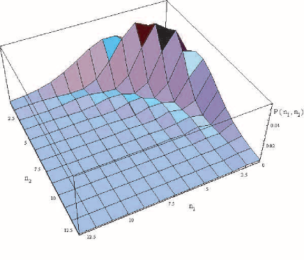
Figure 1: $P(n_{1},n_{2})$ for a two–mode squeezed state, for $r=0.8$, $\beta_{1}=\beta_{2}=3$ and $|\gamma|=0$.

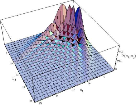
Figure 2: $P(n_{1},n_{2})$ for two–mode squeezed state, for $r=1.5$, $\beta_{1}=\beta_{2}=5$ and $|\gamma|=0$.

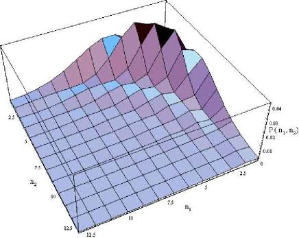
Figure 3: $P(n_{1},n_{2})$ of the four-photon HEMPSS, for $r=0.8$, $\beta_{1}=\beta_{2}=3$ and $|\gamma|=0.1$, $\theta_{1}=\theta_{2}=0$, $\delta_{1}=\delta_{2}=\frac{\pi}{2}$.

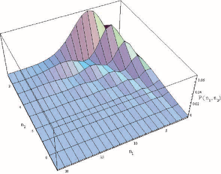
Figure 4: $P(n_{1},n_{2})$ of the four-photon HEMPSS, for $r=0.8$, $\beta_{1}=\beta_{2}=3$ and $|\gamma|=0.1$, $\theta_{1}=\theta_{2}=0$, $\delta_{1}=\pi$, $\delta_{2}=0$.

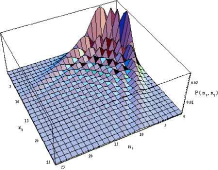
Figure 5: $P(n_{1},n_{2})$ of the four-photon HEMPSS, for $r=1.5$, $\beta_{1}=\beta_{2}=5$ and $|\gamma|=0.1$, $\theta_{1}=\theta_{2}=0$, $\delta_{1}=\delta_{2}=\frac{\pi}{2}$.

We see that the form and the oscillations of the PND for the four-photon HEMPSS strongly depend on the values of the phases $\delta_{1}$ and $\delta_{2}$ which produce competing effects in $U(Z,Z^{{\dagger}})$. In fact, in Figs. 3, 5, 7, 9, corresponding to the symmetric choice for the phases, the PND is symmetric with respect to $n_{1}$ and $n_{2}$. Viceversa, in Figs. 4, 6, 8, 10 the asymmetric choice of the phases leads to an asymmetric PND: the peaks are displaced, and their number and form are changed.

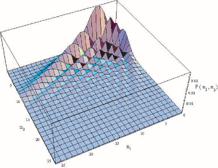
Figure 6: $P(n_{1},n_{2})$ of the four-photon HEMPSS, for $r=1.5$, $\beta_{1}=\beta_{2}=5$ and $|\gamma|=0.1$, $\theta_{1}=\theta_{2}=0$, $\delta_{1}=\pi$, $\delta_{2}=0$.

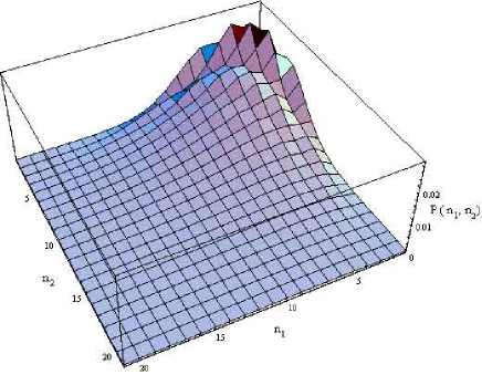
Figure 7: $P(n_{1},n_{2})$ of the four-photon HEMPSS, for $r=0.8$, $\beta_{1}=\beta_{2}=3$ and $|\gamma|=0.2$, $\theta_{1}=\theta_{2}=0$, $\delta_{1}=\delta_{2}=\frac{\pi}{2}$.

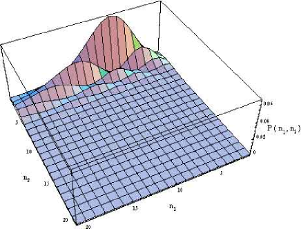
Figure 8: $P(n_{1},n_{2})$ of the four-photon HEMPSS, for $r=0.8$, $\beta_{1}=\beta_{2}=3$ and $|\gamma|=0.2$, $\theta_{1}=\theta_{2}=0$, $\delta_{1}=\pi$, $\delta_{2}=0$.

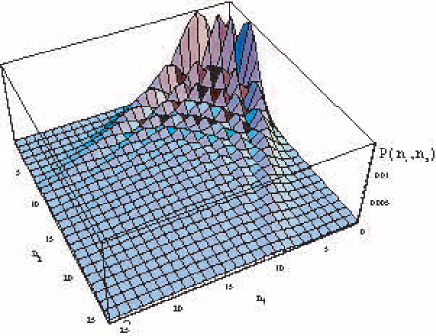
Figure 9: $P(n_{1},n_{2})$ of the four-photon HEMPSS, for $r=1.5$, $\beta_{1}=\beta_{2}=5$ and $|\gamma|=0.2$, $\theta_{1}=\theta_{2}=0$, $\delta_{1}=\delta_{2}=\frac{\pi}{2}$.

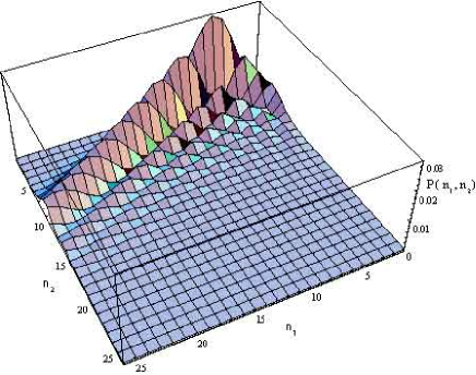
Figure 10: $P(n_{1},n_{2})$ of the four-photon HEMPSS, for $r=1.5$, $\beta_{1}=\beta_{2}=5$ and $|\gamma|=0.2$, $\theta_{1}=\theta_{2}=0$, $\delta_{1}=\pi$, $\delta_{2}=0$.

As for the standard squeezed states, enhancing the squeezing parameter $r$ enhances the oscillations of the PND. The effect of the nonlinear strength $|\gamma|$ is competing with that of $r$. In fact, we see that in Eq. (47) the effective strength $\Delta$ of the nonlinear term involves the product $|\gamma|e^{-r}$, with the choice of parameters yielding $r>0$. Then, a sufficiently high value of $r$ reduces the effect of increasing $|\gamma|$. If we look now at the symmetric PND’s (Figs. 3, 5, 7, 9), we see that, for a high value of $r$, increasing $|\gamma|$ from $0$ to $0.2$ does not change appreciably the oscillations (see Figs. 5, 9 compared with Fig. 2). On the contrary, if $r$ is fixed to a lower value, increasing $|\gamma|$ results in a smoothening of the oscillations (Figs. 3, 7 compared with Fig. 1). Obviously, when $|\gamma|$ attains very high values, it cannot be contrasted by $r$, and the oscillations are even more suppressed. In Figs. 11 and 12 we have plotted the PND for $\beta_{1}=\beta_{2}=0$, and for different values of $r$; this corresponds to the two–mode four–photon squeezed vacuum. As in the case of the standard two–mode squeezed vacuum PND , we obtain a diagonal, symmetric PND, in spite of the unbalanced choice on the phases.

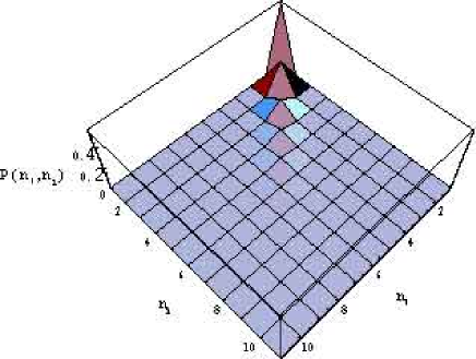
Figure 11: $P(n_{1},n_{2})$ of the four-photon HEMPSS, for $r=0.8$, $\beta_{1}=\beta_{2}=0$ and $|\gamma|=0.1$, $\theta_{1}=\theta_{2}=0$, $\delta_{1}=\pi$, $\delta_{2}=0$.

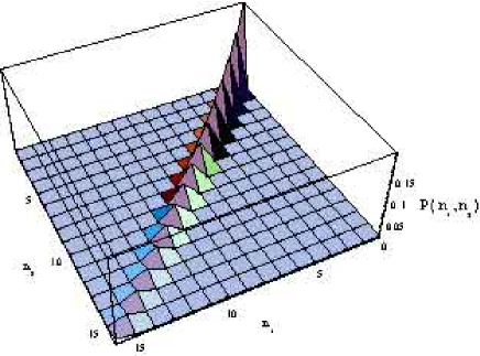
Figure 12: $P(n_{1},n_{2})$ of the four-photon HEMPSS, for $r=1.5$, $\beta_{1}=\beta_{2}=0$ and $|\gamma|=0.2$, $\theta_{1}=\theta_{2}=0$, $\delta_{1}=\pi$, $\delta_{2}=0$.

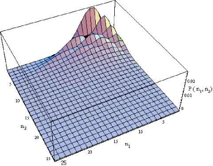
Figure 13: $P(n_{1},n_{2})$ of the four-photon HEMPSS, for $r=0.8$, $\beta_{1}=\beta_{2}=3$ and $|\gamma|=0.2$, $\theta_{1}=-\theta_{2}=\frac{\pi}{6}$, $\delta_{1}=\pi$, $\delta_{2}=0$.

In order to study the influence of the local oscillators angles, in Fig. 13 we have plotted the PND for the same parameters of unbalanced case of Fig. 8, but with $\theta_{1}=-\theta_{2}=\pi/6$; we see that the PND is modified with respect to that of Fig. 8, with a slight re–balancing between the two axes, and less pronounced peaks.

In Figs. 14 and 15 we show the mean numbers of photons in the two modes as a function of $|\gamma|$ for different values of the other parameters. We see that the balanced choice on the phases gives $<n_{1}>=<n_{2}>$ (corresponding to a symmetric PND), and the mean photon numbers increase monotonically with increasing $|\gamma|$. In the unbalanced instance (corresponding to a non symmetric PND), the average photon number in the first mode is markedly larger and monotonically increasing, while the average photon number in the second mode first decreases, and increases monotonically beyond a certain value of $|\gamma|$. This behavior is similar to that exhibited by the HOMPSS for single-mode systems, as discussed in Part I paper1 .

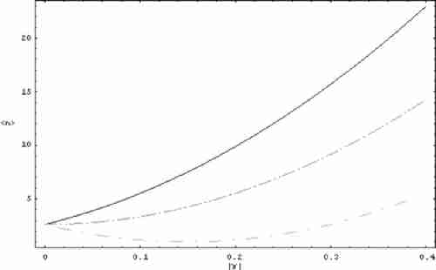
Figure 14: $\langle n_{1}\rangle$ and $\langle n_{2}\rangle$ as a function of $|\gamma|$, for the four-photon HEMPSS, at $r=0.8$, $\beta_{1}=\beta_{2}=3$, $\theta_{1}=\theta_{2}=0$: 1)$\langle n_{1}\rangle$ (full line) and $\langle n_{2}\rangle$ (dot–dashed line) for $\delta_{1}=\pi$, $\delta_{2}=0$; 2)$\langle n_{1}\rangle=\langle n_{2}\rangle$ for $\delta_{1}=\delta_{2}=\frac{\pi}{2}$ (dotted line).

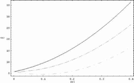
Figure 15: $\langle n_{1}\rangle$ and $\langle n_{2}\rangle$ as a function of $|\gamma|$, for the four-photon HEMPSS, at $r=1.5$, $\beta_{1}=\beta_{2}=5$, $\theta_{1}=\theta_{2}=0$: 1)$\langle n_{1}\rangle$ (full line) and $\langle n_{2}\rangle$ (dot–dashed line) for $\delta_{1}=\pi$, $\delta_{2}=0$; 2)$\langle n_{1}\rangle=\langle n_{2}\rangle$ for $\delta_{1}=\delta_{2}=\frac{\pi}{2}$ (dotted line).

We next study the average photon number for the HEMPSS as a function of the local oscillators angles $\theta_{1}$, $\theta_{2}$, comparing with the case of two–mode squeezed states (Fig. 16). To this aim, when $|\gamma|=0$ we retain as a formal trick the dependence on $\theta_{1}$ and $\theta_{2}$ by fixing $\phi=\theta_{1}+\theta_{2}$, according to canonical conditions Eqs. (21). Because of the choice $\beta_{1}=\beta_{2}$, the plot $\langle n_{1}\rangle=\langle n_{2}\rangle$ is somehow redundant; it is symmetric and shows an oscillatory behavior, as it should be.

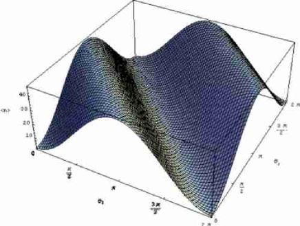
Figure 16: $\langle n_{1}\rangle=\langle n_{2}\rangle$ as a function of $\theta_{1}$ and $\theta_{2}$ ($\phi=\theta_{1}+\theta_{2}$), of a standard two-mode squeezed state ($\gamma=0$), for $r=0.8$, $\beta_{1}=\beta_{2}=3$.

For the nonlinear case, we fix the parameters in the following way: we let $\beta_{1}=\beta_{2}=3$, $r=0.8$ , $|\gamma|=0.4$ and $\delta_{1}=\pi$, $\delta_{2}=\phi$, because of the canonical conditions. As we can see in Figs. 17 and 18, the situation is very different from that of the standard two-mode squeezed states. The shape is strongly deformed and we can observe regions with a suppressed or enhanced number of photons with respect to the mean number of a standard two-mode squeezed state (see Fig. 16).

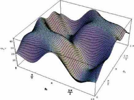
Figure 17: $\langle n_{1}\rangle$ as a function of $\theta_{1}$ and $\theta_{2}$, of the four-photon HEMPSS, for $r=0.8$, $\beta_{1}=\beta_{2}=3$, $|\gamma|=0.4$, $\delta_{1}=\pi$, $\delta_{2}=\phi$.

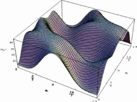
Figure 18: $\langle n_{2}\rangle$ as a function of $\theta_{1}$ and $\theta_{2}$, for the four-photon HEMPSS, at $r=0.8$, $\beta_{1}=\beta_{2}=3$, $|\gamma|=0.4$, $\delta_{1}=\pi$, $\delta_{2}=\phi$.

Finally, we have plotted the second-order two-mode correlation function $g^{(2)}(0)=\langle a_{1}^{\dagger}a_{1}a_{2}^{\dagger}a_{2}\rangle/\langle a_{1}^{\dagger}a_{1}\rangle\langle a_{2}^{\dagger}a_{2}\rangle$ as a function of the local oscillators angles $\theta_{1}$ and $\theta_{2}$. We again obtain a variety of shapes, corresponding to different statistical behaviors. In particular we observe oscillating transitions from bunching to antibunching behaviors. In this case as well, we show for comparison the three-dimensional plot of $g^{(2)}(0)$ for a two–mode squeezed state Fig. 19. It is of course symmetric and exhibits a narrow region of antibunching.

Figure 19: $g^{(2)}(0)$ as a function of $\theta_{1}$ and $\theta_{2}$($\phi=\theta_{1}+\theta_{2}$), for a standard two-mode squeezed state with $\gamma=0$, $r=0.8$, $\beta_{1}=\beta_{2}=3$.

Already for small strengths of the nonlinearity ($|\gamma|=0.1$) we can see from Fig. 20 that the shape of the correlation function is deformed with respect to that of the two-mode squeezed state. This deformation becomes more marked for larger values of $|\gamma|$, as shown in Figs. 22 and 23. From Fig. 21 we see that for increasing values of the squeezing parameter, the antibunching behavior is attenuated and the effect of the nonlinearity is progressively suppressed. This is a further indication of the competing effects of the squeezing and of the nonlinearity.

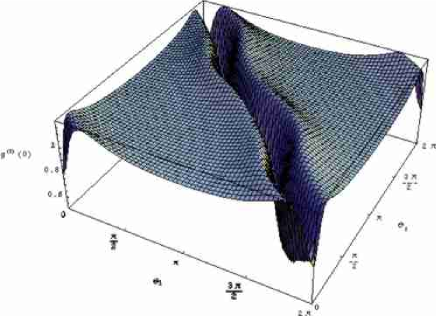
Figure 20: $g^{(2)}(0)$ as a function of $\theta_{1}$ and $\theta_{2}$, for the four-photon HEMPSS, at $r=0.8$, $\beta_{1}=\beta_{2}=3$, $|\gamma|=0.1$, $\delta_{1}=\pi$, and $\delta_{2}=\phi$.

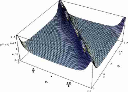
Figure 21: $g^{(2)}(0)$ as a function of $\theta_{1}$ and $\theta_{2}$, for the four-photon HEMPSS, at $r=1.5$, $\beta_{1}=\beta_{2}=5$, $|\gamma|=0.1$, $\delta_{1}=\pi$, and $\delta_{2}=\phi$.

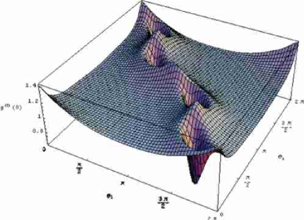
Figure 22: $g^{(2)}(0)$ as a function of $\theta_{1}$ and $\theta_{2}$, for the four-photon HEMPSS, at $r=0.8$, $\beta_{1}=\beta_{2}=3$, $|\gamma|=0.2$, $\delta_{1}=\pi$, and $\delta_{2}=\phi$.

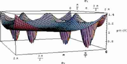
Figure 23: $g^{(2)}(0)$ as a function of $\theta_{1}$ and $\theta_{2}$, for the four-photon HEMPSS, with $r=0.8$, $\beta_{1}=\beta_{2}=3$, $|\gamma|=0.2$, $\delta_{1}=\pi$, and $\delta_{2}=\phi$.

Summing up, similarly the case of single-mode systems, we observe that the photon statistics of the two-mode, four-photon HEMPSS can be strongly modified by the gauging of the parameters entering the nonlinear canonical transformations, such as the heterodyne mixing angles $\theta_{1}$ and $\theta_{2}$, the strength $|\gamma|$, and the phases $\delta_{1}$ and $\delta_{2}$ of the nonlinearity. Let us notice that this flexibility can be further enhanced by considering the large number of different possible canonical choices for the parameters that have not been explored in the present work.

VII Quantum dynamics in nonlinear media and generation of the HEMPSS

The interaction part of the Hamiltonian Eq. (22) contains many non degenerate and degenerate multiphoton terms; this complex structure is evidently due to the non trivial canonical constraints associated to the structure of the nonlinear Bogoliubov transformations. On the other hand, the very existence of a canonical structure suggests that the experimental realization of the associated multiphoton processes and squeezed states should be conceivable. To this aim, we must bear in mind that any experimental realization of the HEMPSS must necessarily involve high order contributions to the susceptibility in nonlinear media. In this Section we briefly review the essential features of the theory of macroscopic quantum electrodynamics in nonlinear media, referring for a more exhaustive treatment to Shen ; Tucker ; Hillery . The standard approach is the phenomenological quantization of the classical macroscopic theory. The macroscopic description of the interaction of the electromagnetic field with matter is based on the polarization vector Bloembergen1 ; Bloembergen2 ; Butcher

$$P_{i} = \underline{\chi}^{(1)}:\overline{E}+\underline{\chi}^{(2)}:\overline{E}\overline{E}+\underline{\chi}^{(3)}:\overline{E}\overline{E}\overline{E}+...\;$$ (51)

$$= \chi^{(1)}\delta_{ij}E_{j}+\chi^{(2)}_{ijk}E_{j}E_{k}+\chi^{(3)}_{ijkl}E_{j}E_{k}E_{l}+...$$

where $\overline{E}$ is the electric field, $\chi_{ijkl...}^{(n)}$ is the ($n+1)--th$ rank susceptibility tensor and the subscripts indicate the spatial and polarization components. For a lossless, nondispersive and uniform medium, the susceptibilities $\underline{\chi}^{(n)}$ are symmetric tensors. Considering only electric dipole interactions, the electric contribution to the electromagnetic energy in the nonlinear medium is

$$H=\int_{V}d^{3}r\left[\frac{1}{2}\varepsilon_{0}E^{2}(\overline{r},t)+\sum_{n}X_{n}(\overline{r})\right]\;,$$ (52)

where

$$X_{n}(\overline{r})=\frac{n\varepsilon_{0}}{n+1}\underline{\chi}^{(n)}:\overline{E}\overline{E}...\overline{E}\;.$$ (53)

In terms of the Fourier components of the field,

$$X_{n}=\frac{n\varepsilon_{0}}{n+1}\int\prod_{l=1}^{n+1}d\omega_{l}e^{-i\omega_{l}t}$$

$$\cdot\underline{\chi}^{(n)}(\omega_{2},...,\omega_{n+1}):\overline{E}\overline{E}...\overline{E}\;.$$ (54)

In deriving Eq. (54), it is tacitly assumed that $\chi^{n}(\omega)$ is independent on the wave-vector $\overline{k}$ (electric dipole approximation), that in the electromagnetic energy of the medium terms of order $\omega\partial\chi^{(n)}/\partial\omega$ can be ignored, and that nonlinearities are small.

The canonical quantization of the macroscopic field in a nonlinear medium is introduced by replacing the classical field $\overline{E}(\overline{r},t)$ with the corresponding free-field Hilbert space operator

$$\textbf{E}(\overline{r},t) = i\sum_{\overline{k},\lambda}\left[\frac{\hbar\omega_{\overline{k},\lambda}}{2\varepsilon_{0}V}\right]^{1/2}\{a_{\overline{k},\lambda}\epsilon_{\overline{k},\lambda}e^{i(\overline{k}\cdot\overline{r}-\omega_{\overline{k},\lambda}t)}$$

$$-a_{\overline{k},\lambda}^{{\dagger}}\epsilon_{\overline{k},\lambda}^{*}e^{-i(\overline{k}\cdot\overline{r}-\omega_{\overline{k},\lambda}t)}\}\;,$$

where $V$ is the spatial volume, $\epsilon_{\overline{k},\lambda}$ is the unit vector encoding the wave-vector $\overline{k}$ and the polarization $\lambda$, $\omega_{\overline{k},\lambda}=c|\overline{k}|/n_{\overline{k},\lambda}$ is the angular frequency in the medium ($n_{\overline{k},\lambda}$ being the index of refraction), and $a_{\overline{k},\lambda}$ is the corresponding boson annihilation operator. Denoting by $\bf{k}$ the pair ($\overline{k},\lambda$), and defining

$$\Lambda_{\textbf{k}}=\sqrt{\frac{\hbar\omega_{\bf{k}}}{2\varepsilon_{0}V}}\;,$$ (56)

the Fourier components of the quantum field are given by

$$\textbf{E}(\omega) = i\sum_{\bf{k}}\Lambda_{\textbf{k}}\{a_{\bf{k}}\epsilon_{\bf{k}}e^{i{\overline{k}}\cdot{\overline{r}}}\delta(\omega-\omega_{\bf{k}})$$ (57)

$$-a_{\bf{k}}^{{\dagger}}\epsilon_{\bf{k}}^{*}e^{-i{\overline{k}}\cdot{\overline{r}}}\delta(\omega+\omega_{\bf{k}})\}\;.$$

The contribution of the $n$–th order nonlinearity to the quantum Hamiltonian can thus be obtained by replacing the Fourier components of the quantum field Eq. (57) in Eq. (54). Owing to the phase factors $e^{i\omega t}$, many of the terms resulting from the Eq. (54) are rapidly oscillating and average to zero; they can then be neglected in the rotating wave approximation. The surviving terms correspond to sets of frequencies that, due to the constraint of energy conservation, satisfy the relation

$$\sum_{i=1}^{s}\omega_{\bf{k}_{i}}=\sum_{i=s+1}^{n+1}\omega_{\bf{k}_{i}}\;,$$ (58)

and involve products of boson operators of the form

$$a_{\bf{k}_{1}}a_{\bf{k}_{2}}\cdot\cdot\cdot a_{\bf{k}_{r}}a_{\bf{k}_{r+1}}^{{\dagger}}\cdot\cdot\cdot a_{\bf{k}_{n+1}}^{{\dagger}}\;,$$ (59)

and their hermitian conjugates. The occurrence of a particular multiphoton process is selected by imposing the conservation of momentum. This is the so-called phase matching condition and, classically, corresponds to the synchronism of the phase velocity of the electric field and of the polarization waves. These conditions can be realized by exploiting the birefringent and dispersion properties of anisotropic crystals.

The relevant modes of the radiation involved in a nonlinear parametric process can be determined by the condition Eq. (58) and the corresponding phase-matching condition

$$\sum_{i=1}^{s}{{\overline{k}}}_{i}=\sum_{i=s+1}^{n+1}{{\overline{k}}}_{i}\;.$$ (60)

We will have to consider in detail the terms of the quantized Hamiltonian Eq. (52) up to the fifth-order contribution to the susceptibility tensor ($n=5$), using the expansion Eq. (57) and assuming the matching conditions Eqs. (58) and (60). These terms are needed to generate the processes described by the Hamiltonian Eq. (22) and the associated HEMPSS, and are listed in Appendix A.

VIII Experimental setups

VIII.1 Realizing the two–mode four–photon Hamiltonian

We now specialize to a possible, but by no means unique, experimental setup the previous general results in the context of a multiple parametric approximation, in order to realize the particular multiphoton processes described by the two–mode Hamiltonians Eq. (22).

We consider a nonlinear crystal, illuminated by twelve laser pumps at different frequencies :

$$E^{(+)}=\sum_{i=1}^{12}E_{i}e^{-i(\Omega_{i}t-\bf{k_{i}}\cdot\bf{r})}\,.$$ (61)

We assume a lossless, nondispersive, uniform, noncentrosymmetric medium, in order to exploit the properties of spatial and Kleinman symmetry of the susceptibility tensors, which can be taken to be real. Due to the high intensity of the lasers, all the pump fields are treated classically in this model. For simplicity, we will assume a single polarization of the light, and unidirectional propagating waves. Two quantum modes of the radiation field, respectively at incommensurate frequencies $\omega_{1}$ and $\omega_{2}$, are excited in the parametric processes in the nonlinear crystal. We impose the following relations on the frequencies of the laser pumps :

$$\Omega_{1}+\Omega_{2}=\omega_{1}+\omega_{2}\;,\;\quad\Omega_{3}+\Omega_{4}=2(\omega_{1}+\omega_{2})\,,$$

$$\Omega_{5}+\Omega_{6}=3\omega_{1}\;,\;\quad\Omega_{7}+\Omega_{8}=3\omega_{2}\,,$$

$$\Omega_{9}+\Omega_{10}=2\omega_{1}-\omega_{2}\,,\;\;\Omega_{11}+\Omega_{12}=2\omega_{2}-\omega_{1}\,,$$ (62)

with the corresponding phase-matching conditions. With this choice, given $\omega_{1}$ and $\omega_{2}$, each pair of frequencies is fixed by the corresponding phase matching condition. With a sufficiently large number of laser pumps, many related independent equations can be satisfied. Reducing the number of pumps and of independent equations is certainly possible, at the price of leading to more complicated relations between the frequencies.

The introduction of several pumps, with suitable frequencies, allows to study the multiphoton processes corresponding to higher-order contributions to the susceptibility tensor. We will use conditions Eqs. (62) to obtain two-, three- and four- photon down conversion processes, and the associated mixed processes in the interacting Hamiltonian. We write all the contributions considered in our model in the interaction representation. Let us denote by $\kappa^{js}_{lm}$ the coefficient of the generic interaction term $a_{1}^{{\dagger}j}a_{2}^{{\dagger}s}a_{1}^{l}a_{2}^{m}$, describing the creation of $j$ photons and the annihilation of $l$ photons in the first mode, and the creation of $s$ photons and the annihilation of $m$ photons in the second mode. The two–photon down conversion term due to third-order interaction reads:

$$H_{2}=\kappa^{11}_{00}a_{1}^{{\dagger}}a_{2}^{{\dagger}}E_{1}E_{2}+h.c.\,,$$ (63)

with

$$\kappa^{11}_{00}\propto\chi^{(3)}(-\Omega_{2};-\omega_{1},-\omega_{2},\Omega_{1}).$$

The degenerate three–photon down conversion terms are

$$H_{3d}=(\kappa^{30}_{00}a_{1}^{{\dagger}3}E_{5}E_{6}+h.c.)+(\kappa^{03}_{00}a_{2}^{{\dagger}3}E_{7}E_{8}+h.c.)\,,$$ (64)

with

$$\kappa^{30}_{00}\propto\chi^{(4)}(-\Omega_{6};-\omega_{1},-\omega_{1},-\omega_{1},\Omega_{5})\,,$$

and

$$\kappa^{03}_{00}\propto\chi^{(4)}(-\Omega_{8};-\omega_{2},-\omega_{2},-\omega_{2},\Omega_{7})\,.$$

The semi-degenerate four-photon down conversion term is given by:

$$H_{4sd}=\kappa^{22}_{00}a_{1}^{{\dagger}2}a_{2}^{{\dagger}2}E_{3}E_{4}+h.c.\,,$$ (65)

with

$$\kappa^{22}_{00}\propto\chi^{(5)}(-\Omega_{4};-\omega_{1},-\omega_{1},-\omega_{2},-\omega_{2},\Omega_{3})\,.$$

The semi-degenerate three-photon terms are

$$H_{3sd}=\kappa^{21}_{00}a_{1}^{{\dagger}2}a_{2}E_{9}E_{10}+h.c.\,,$$

$$H^{{}^{\prime}}_{3sd}=\kappa^{12}_{00}a_{2}^{{\dagger}2}a_{1}E_{11}E_{12}+h.c.\,,$$ (66)

where

$$\kappa^{21}_{00}\propto\chi^{(4)}(-\Omega_{10};-\omega_{1},-\omega_{1},\omega_{2},\Omega_{9})\,,$$

and

$$\kappa^{12}_{00}\propto\chi^{(4)}(-\Omega_{12};-\omega_{2},-\omega_{2},\omega_{1},\Omega_{11})\;.$$

In spite of their weaker contributions, we retain for convenience the terms

$$H_{r} =(\kappa^{21}_{10}a_{1}^{{\dagger}2}a_{2}^{{\dagger}}a_{1}E_{1}E_{2}+h.c.)$$ (67)

$$+(\kappa^{12}_{01}a_{1}^{{\dagger}}a_{2}^{{\dagger}2}a_{2}E_{1}E_{2}+h.c.)\,,$$

with

$$\kappa^{21}_{10}\propto\chi^{(5)}(-\Omega_{2};-\omega_{1},-\omega_{2},-\omega_{1},\omega_{1},\Omega_{1})\,,$$

and

$$\kappa^{12}_{01}\propto\chi^{(5)}(-\Omega_{2};-\omega_{1},-\omega_{2},-\omega_{2},\omega_{2},\Omega_{1})\,.$$

Finally, we have to consider the Kerr contributions

$$H_{kerr}=\kappa^{20}_{20}a_{1}^{{\dagger}2}a_{1}^{2}+\kappa^{02}_{02}a_{2}^{{\dagger}2}a_{2}^{2}+\kappa^{11}_{11}a_{1}^{{\dagger}}a_{2}^{{\dagger}}a_{1}a_{2}\,,$$ (68)

where

$$\kappa^{20}_{20}\propto\chi^{(3)}(-\omega_{1};-\omega_{1},-\omega_{1},\omega_{1})\,,$$

$$\kappa^{02}_{02}\propto\chi^{(3)}(-\omega_{2};-\omega_{2},-\omega_{2},\omega_{2})\,,$$

and

$$\kappa^{11}_{11}\propto\chi^{(3)}(-\omega_{2};-\omega_{1},\omega_{1},-\omega_{2})\,.$$

In conclusion, the full interaction Hamiltonian reads

$$H_{I}=H_{2}+H_{3d}+H_{4sd}+H_{3sd}+H^{{}^{\prime}}_{3sd}+H_{r}+H_{kerr}\,\,.$$ (69)

We stress again that our choice is only one of the many possible ones. One could envisage different configurations, using nonlinear crystals of particular anisotropy classes, and choosing different polarizations for the two quantum modes.

Let us consider the interaction part of the Hamiltonian Eq. (22). We see that all its terms are included in Eq. (69), and that the two Hamiltonians coincide if we impose the equality of the corresponding coefficients and assume

$$\kappa^{20}_{20}\approx\kappa^{02}_{02}\approx 2\kappa^{11}_{11}\,.$$ (70)

Equality of the coefficients can be realized by tuning the complex amplitudes of the classical fields.

VIII.2 Generating the four-photon HEMPSS

Eqs. (43) and (48) suggest a possible method to realize experimentally the HEMPSS Eq. (36) for the simplest, quadratic nonlinearity. Adopting the same criteria of Subsection VIII.1, we consider again a sample nonlinear crystal, illuminated by eight classical pumps at different frequencies

$$E^{(+)}=\sum_{i=1}^{8}E_{i}e^{-i(\Omega_{i}t-\bf{k_{i}}\cdot\bf{r})}\,.$$ (71)

We impose the following relations

$$\Omega_{1}+\Omega_{2}=3\omega_{1}\,,\,\quad\Omega_{3}+\Omega_{4}=3\omega_{2}\,,$$

$$\Omega_{5}+\Omega_{6}=2\omega_{1}-\omega_{2}\,,\;\;\;\Omega_{7}+\Omega_{8}=2\omega_{2}-\omega_{1}\,,$$ (72)

and collinear phase-matching conditions. We then obtain an interaction Hamiltonian of the form

$$H_{I}=\kappa^{30}_{00}a_{1}^{{\dagger}3}E_{1}E_{2}+\kappa^{03}_{00}a_{2}^{{\dagger}3}E_{3}E_{4}$$

$$+\kappa^{20}_{01}a_{1}^{{\dagger}2}a_{2}E_{5}E_{6}+\kappa^{02}_{10}a_{2}^{{\dagger}2}a_{1}E_{7}E_{8}+h.c.\,,$$ (73)

with

$$\kappa^{30}_{00}\propto\chi^{(4)}(-\Omega_{2};-\omega_{1},-\omega_{1},-\omega_{1},\Omega_{1})\,,$$

$$\kappa^{03}_{00}\propto\chi^{(4)}(-\Omega_{4};-\omega_{2},-\omega_{2},-\omega_{2},\Omega_{3})\,,$$

$$\kappa^{20}_{01}\propto\chi^{(4)}(-\Omega_{6};-\omega_{1},-\omega_{1},\omega_{2},\Omega_{5})\,,$$

$$\kappa^{02}_{10}\propto\chi^{(4)}(-\Omega_{8};-\omega_{2},-\omega_{2},\omega_{1},\Omega_{7})\,,$$

where we have neglected the Kerr terms, due to their weaker contributions.

Tuning the intensities of the external pumps, one can force the Hamiltonian Eq. (73) to coincide with the interaction terms appearing in the exponent of Eq. (48). The unitary operator Eq. (48) can thus be realized by the Hamiltonian unitary evolution $e^{-itH_{I}}$, and the HEMPSS can be generated by imposing this unitary Hamiltonian evolution on a standard two–mode squeezed state.

IX Conclusions

In this paper we define a canonical formalism for two–mode multiphoton processes. We achieve this goal exploiting generalized, nonlinear two–mode Bogoliubov transformations. These transformations are defined by introducing a largely arbitrary, nonlinear function of a heterodyne superposition of the fundamental mode operators, depending on two local oscillator angles (heterodyne mixing angles). The nonlinear transformations are canonical once simple algebraic constraints, analogous to those holding for the linear Bogoliubov transformations, are imposed on the complex coefficients of the nonlinear mapping. The scheme generalizes the one introduced in the companion paper (Part I) paper1 . Among the possible choices of the nonlinear function we pay special attention to those associated to arbitrary $n-th$ powers of the heterodyne variables. This class of transformations defines canonical Hamiltonian models of $2n$–photons nondegenerate and degenerate processes. We have determined the common eigenstates of the transformed operators, and found their explicit form in the entangled state representation. These states form an overcomplete set and exhibit coherence and squeezing properties. They are non–Gaussian, entangled multiphoton states of bipartite systems. They can be defined as well by applying on the two-mode squeezed vacuum an unitary operator with nonlinear exponent that realizes a heterodyne mixing of the fundamental modes. We have thus named these states Heterodyne Multiphoton Squeezed States (HEMPSS). For quadratic nonlinearities, the HEMPSS realize a two–mode version of the cubic phase states bartlett . Thus the HEMPSS are potentially interesting candidates for schemes of quantum communication, and for the implementation of continuous variable quantum computing involving multiphoton processes. One of the most appealing features of the HEMPSS concerns the study of their statistical properties. As in the single-mode case, but with even more striking effects, the statistics can be largely gauged by tuning the strength and the phases of the nonlinear interaction, and the local oscillator (heterodyne mixing) angles. For the case of lowest (quadratic) nonlinearity, we investigate possible routes to the experimental realization of canonical multiphoton Hamiltonians, and the generation of the associated HEMPSS. Our proposal relies on the use of higher-order contributions to the susceptibility in nonlinear media, and on the engineering of suitable classical pumps and phase–matching conditions.

In future work we intend to qualify and quantify the entanglement of the HEMPSS, and their possible use in the framework of the continuous variables universal quantum computation. The overcompleteness of the HEMPSS allows in principle to study the unitary evolutions ruled by any diagonalizable Hamiltonian associated to a quadratic nonlinearity, and by other Hamiltonian operators associated to known group structures in terms of the transformed mode variables. In this way, we intend to introduce and characterize other classes of nonclassical multiphoton states amenable to analytic study.

Appendix A

a) $X_{2}$ contribution

We fix the frequencies $\omega_{\bf{k}_{1}}$, $\omega_{\bf{k}_{2}}$, $\omega_{\bf{k}_{3}}$ such that $\omega_{\bf{k}_{1}}=\omega_{\bf{k}_{2}}+\omega_{\bf{k}_{3}}$. Ignoring the oscillating terms, we obtain

$$\int_{V}d^{3}rX_{2}(\bf{r})=\frac{2}{3}\varepsilon_{0}\int_{V}d^{3}r\int(\prod_{l=1}^{3}d\omega_{l}e^{-i\omega_{l}t})$$

$$\cdot\underline{\chi}^{(2)}(\omega_{2},\omega_{3}):\textbf{E}(\omega_{1})\textbf{E}(\omega_{2})\textbf{E}(\omega_{3})\simeq$$

$$2i\varepsilon_{0}\sum_{\bf{k}_{1},\bf{k}_{2},\bf{k}_{3}}\Lambda_{\bf{k}_{1}}\Lambda_{\bf{k}_{2}}\Lambda_{\bf{k}_{3}}\underline{\chi}^{(2)}(\omega_{\bf{k}_{2}},\omega_{\bf{k}_{3}}):\epsilon_{\bf{k}_{1}}^{*}\epsilon_{\bf{k}_{2}}\epsilon_{\bf{k}_{3}}$$

$$\cdot a_{\bf{k}_{1}}^{{\dagger}}a_{\bf{k}_{2}}a_{\bf{k}_{3}}\int_{V}d^{3}re^{-i(\bf{k}_{1}-\bf{k}_{2}-\bf{k}_{3})\cdot\bf{r}}+h.c.$$ (74)

Condition Eq. (60) eliminates the strong dependence on the phase mismatch $\Delta\bf{k}=\bf{k}_{1}-\bf{k}_{2}-\bf{k}_{3}$ of the volume integral Eq. (74).

The resulting nonlinear parametric processes (in a three wave interaction) are described by a Hamiltonian of the form

$$H\propto\chi^{(2)}a^{{\dagger}}bc+h.c.\;,\;$$ (75)

where $a$, $b$, $c$ are three different modes at frequency $\omega_{a}$, $\omega_{b}$, $\omega_{c}$, respectively. Hamiltonian Eq. (75) can describe: sum-frequency mixing for input $b$ and $c$ and $\omega_{a}=\omega_{b}+\omega_{c}$; non-degenerate parametric amplification for input $a$, and $\omega_{a}=\omega_{b}+\omega_{c}$; difference-frequency mixing for input $a$ and $c$ and $\omega_{b}=\omega_{c}-\omega_{a}$.

If some of the modes in Hamiltonian Eq. (75) degenerate in the same mode (i.e. at the same frequency, wave vector and polarization), one obtains degenerate parametric processes as : second harmonic generation for input $b=c$ and $\omega_{a}=2\omega_{b}$; degenerate parametric amplification for input $a$, and $\omega_{a}=2\omega_{b}$, with $b=c$; other effects as optical rectification and Pockels effect involving d.c. fields.

b) $X_{3}$ contribution

We must now consider

$$\int_{V}d^{3}rX_{3}(\bf{r})=\frac{3}{4}\varepsilon_{0}\int_{V}d^{3}r\int\ \prod_{l=1}^{4}d\omega_{l}e^{-i\omega_{l}t}$$

$$\cdot\underline{\chi}^{(3)}(\omega_{2},\omega_{3},\omega_{4}):\textbf{E}(\omega_{1})\textbf{E}(\omega_{2})\textbf{E}(\omega_{3})\textbf{E}(\omega_{4})\,.$$ (76)

In this case, the relation Eq. (58) splits in the two distinct conditions

$$\omega_{\bf{k}_{1}}=\omega_{\bf{k}_{2}} + \omega_{\bf{k}_{3}}+\omega_{\bf{k}_{4}}\,,\;$$ (77)

$$\omega_{\bf{q}_{1}}+\omega_{\bf{q}_{2}} = \omega_{\bf{q}_{3}}+\omega_{\bf{q}_{4}}\;,\;$$ (78)

and the interaction Hamiltonian term takes the form

$$H\propto[\alpha\chi^{(3)}(\omega_{\bf{k}_{2}},\omega_{\bf{k}_{3}},\omega_{\bf{k}_{4}})a_{\bf{k}_{1}}^{{\dagger}}a_{\bf{k}_{2}}a_{\bf{k}_{3}}a_{\bf{k}_{4}}+h.c.]+$$

$$[\beta\chi^{(3)}(-\omega_{\bf{q}_{2}},\omega_{\bf{q}_{3}},\omega_{\bf{q}_{4}})a_{\bf{q}_{1}}^{{\dagger}}a_{\bf{q}_{2}}^{{\dagger}}a_{\bf{q}_{3}}a_{\bf{q}_{4}}+h.c.]\;,\;$$ (79)

where $\alpha$, $\beta$ are $c$-numbers, and $a_{\bf{k}_{i}}$ ($i=1,..,4$) are four different modes at frequency $\omega_{\bf{k}_{i}}$.

This term can give origin to a great variety of effects such as high order harmonic generation, Kerr effect etc.

c) $X_{4}$ contribution

We manage now the term

$$\int_{V}d^{3}rX_{4}(\bf{r})=\frac{4}{5}\varepsilon_{0}\int_{V}d^{3}r\int\prod_{l=1}^{5}d\omega_{l}e^{-i\omega_{1}t}\;$$

$$\cdot\underline{\chi}^{(4)}(\omega_{2},\omega_{3},\omega_{4},\omega_{5}):\textbf{E}(\omega_{1})\textbf{E}(\omega_{2})\textbf{E}(\omega_{3})\textbf{E}(\omega_{4})\textbf{E}(\omega_{5})\;.$$

Also in this case the relation (58) gives two independent conditions:

$$\omega_{\bf{k}_{1}}=\omega_{\bf{k}_{2}} + \omega_{\bf{k}_{3}}+\omega_{\bf{k}_{4}}+\omega_{\bf{k}_{5}}\;\,,$$ (81)

$$\omega_{\bf{q}_{1}}+\omega_{\bf{q}_{2}} = \omega_{\bf{q}_{3}}+\omega_{\bf{q}_{4}}+\omega_{\bf{q}_{5}}\;,\;$$ (82)

while the corresponding Hamiltonian contribution has a more complex structure with multimode interactions:

$$H\propto[\delta\chi^{(4)}(\omega_{\bf{k}_{2}},\omega_{\bf{k}_{3}},\omega_{\bf{k}_{4}},\omega_{\bf{k}_{5}})a_{\bf{k}_{1}}^{{\dagger}}a_{\bf{k}_{2}}a_{\bf{k}_{3}}a_{\bf{k}_{4}}a_{\bf{k}_{5}}$$

$$+\gamma\chi^{(4)}(-\omega_{\bf{q}_{2}},\omega_{\bf{q}_{3}},\omega_{\bf{q}_{4}},\omega_{\bf{q}_{5}})a_{\bf{q}_{1}}^{{\dagger}}a_{\bf{q}_{2}}^{{\dagger}}a_{\bf{q}_{3}}a_{\bf{q}_{4}}a_{\bf{q}_{5}}+h.c.]\,.$$

(83)

Here $\delta$, $\gamma$ are $c$-numbers, and $a_{\bf{k}_{i}}$ ($i=1,..5$) are five different modes at frequency $\omega_{\bf{k}_{i}}$.

d) $X_{5}$ contribution

At last we consider the term

$$\int_{V}d^{3}rX_{5}(\bf{r})=$$

$$\frac{5}{6}\varepsilon_{0}\int_{V}d^{3}r\int\prod_{l=1}^{6}d\omega_{l}e^{-i\omega_{1}t}\underline{\chi}^{(5)}(\omega_{2},\omega_{3},\omega_{4},\omega_{5},\omega_{6}):\;$$

$$\textbf{E}(\omega_{1})\textbf{E}(\omega_{2})\textbf{E}(\omega_{3})\textbf{E}(\omega_{4})\textbf{E}(\omega_{5})\textbf{E}(\omega_{6})\;.$$ (84)

In this case the relation (58) gives three conditions:

$$\omega_{\bf{k}_{1}}=\omega_{\bf{k}_{2}} + \omega_{\bf{k}_{3}}+\omega_{\bf{k}_{4}}+\omega_{\bf{k}_{5}}+\omega_{\bf{k}_{6}}\,,$$ (85)

$$\omega_{\bf{q}_{1}}+\omega_{\bf{q}_{2}} = \omega_{\bf{q}_{3}}+\omega_{\bf{q}_{4}}+\omega_{\bf{q}_{5}}+\omega_{\bf{q}_{6}}\,,$$ (86)

$$\omega_{\bf{p}_{1}}+\omega_{\bf{p}_{2}} + \omega_{\bf{p}_{3}}=\omega_{\bf{p}_{4}}+\omega_{\bf{p}_{5}}+\omega_{\bf{p}_{6}}\;.$$ (87)

The corresponding Hamiltonian contribution is:

$$H\propto[\eta_{1}\chi^{(5)}(\omega_{\bf{k}_{2}},\omega_{\bf{k}_{3}},\omega_{\bf{k}_{4}},\omega_{\bf{k}_{5}},\omega_{\bf{k}_{6}})a_{\bf{k}_{1}}^{{\dagger}}a_{\bf{k}_{2}}a_{\bf{k}_{3}}a_{\bf{k}_{4}}a_{\bf{k}_{5}}a_{\bf{k}_{6}}$$

$$+\eta_{2}\chi^{(5)}(-\omega_{\bf{q}_{2}},\omega_{\bf{q}_{3}},\omega_{\bf{q}_{4}},\omega_{\bf{q}_{5}},\omega_{\bf{q}_{6}})a_{\bf{q}_{1}}^{{\dagger}}a_{\bf{q}_{2}}^{{\dagger}}a_{\bf{q}_{3}}a_{\bf{q}_{4}}a_{\bf{q}_{5}}a_{\bf{q}_{6}}$$

$$+\eta_{3}\chi^{(5)}(-\omega_{\bf{p}_{2}},-\omega_{\bf{p}_{3}},\omega_{\bf{p}_{4}},\omega_{\bf{p}_{5}},\omega_{\bf{p}_{6}})a_{\bf{p}_{1}}^{{\dagger}}a_{\bf{p}_{2}}^{{\dagger}}a_{\bf{p}_{3}}^{{\dagger}}a_{\bf{p}_{4}}a_{\bf{p}_{5}}a_{\bf{p}_{6}}$$

$$+h.c.]$$ (88)

Here $\eta_{i}$ ($i=1,2,3$) are $c$-numbers, and $a_{\bf{k}_{i}}$ ($i=1,..6$) are six different modes at frequency $\omega_{\bf{k}_{i}}$.

References

• (1) F. Dell’Anno, S. De Siena, and F. Illuminati, “Structure of multiphoton quantum optics. I. Canonical formalism and homodyne squeezed states”, LANL preprint quant–ph/0308081 (2003).
• (2) H. P. Yuen, Phys. Rev. A 13, 2226 (1976).
• (3) C. M. Caves and B. L. Schumaker, Phys. Rev. A 31, 3068 (1985); B. L. Schumaker and C. M. Caves, Phys. Rev. A 31, 3093 (1985).
• (4) J. H. Shapiro and S. S. Wagner, IEEE J. Quantum Electron. QE-20 , 803 (1984).
• (5) H. P. Yuen and J. H. Shapiro, IEEE Trans. Inf. Theory IT-26, 78 (1980).
• (6) FanHong-yi and J. R. Klauder, Phys. Rev. A 49, 704 (1994).
• (7) FanHong-yi and FanYue, Phys. Rev. A 54, 958 (1996).
• (8) G. M. D’Ariano and M. F. Sacchi, Phys. Rev. A 52, R4309 (1995).
• (9) Hongyi Fan, Phys. Rev. A 65, 064102 (2002).
• (10) J. R. Klauder and B.-S. Skagerstam, Coherenct States - Applications in Physics and mathematical Physics (World Scientific, Singapore, 1985).
• (11) A. Perelomov, Generalized Coherent States and Their Applications (Springer Verlag, Heidelberg, 1986); W.-M. Zhang, D. H. Feng, and R. Gilmore, Rev. Mod. Phys. 62, 867 (1990).
• (12) C. M. Caves, C. Zhu, G. J. Milburn, and W. Schleich, Phys. Rev. A 43, 3854 (1991); G. Schrade, V. M. Akulin, V. I. Man’ko, and W. P. Schleich, Phys. Rev. A 48, 2398 (1993).
• (13) W. Schleich and W. A. Wheeler, Nature (London) 326, 574 (1987).
• (14) Y. R. Shen, Phys. Rev. 155, 921 (1967).
• (15) J. Tucker and D. F. Walls, Phys. Rev. 178, 2036 (1969).
• (16) M. Hillery and L. D. Mlodinow, Phys. Rev. A 30, 1860 (1984).
• (17) J. A. Armstrong, N. Bloembergen, J. Ducuing, and P. S. Pershan, Phys. Rev. 127, 1918 (1962).
• (18) N. Bloembergen, Nonlinear Optics, (Benjamin, New York, 1965); R. W. Boyd, Nonlinear Optics (Academic Press, 2002).
• (19) P. N. Butcher and D. Cotter, The Elements of Nonlinear Optics, (Cambridge Univ. Press, 1990).
• (20) S. D. Bartlett and B. C. Sanders, Phys. Rev. A 65, 042304 (2002).