Quantum dynamical correlations:
Effective potential analytic continuation approach

Abstract

We propose a new quantum dynamics method called the effective potential analytic continuation (EPAC) to calculate the real time quantum correlation functions at finite temperature. The method is based on the effective action formalism which includes the standard effective potential. The basic notions of the EPAC are presented for a one-dimensional double well system in comparison with the centroid molecular dynamics (CMD) and the exact real time quantum correlation function. It is shown that both the EPAC and the CMD well reproduce the exact short time behavior, while at longer time their results deviate from the exact one. The CMD correlation function damps rapidly with time because of ensemble dephasing. The EPAC correlation function, however, can reproduce the long time oscillation inherent in the quantum double well systems. It is also shown that the EPAC correlation function can be improved toward the exact correlation function by means of the higher order derivative expansion of the effective action.

I INTRODUCTION

The imaginary time path integral fh provides the quantum statistical mechanical formalism of useful numerical methods for quantum many-body systems. Static observables in such systems have successfully been calculated by the path integral Monte Carlo (PIMC) or path integral molecular dynamics (PIMD) calculation bt ; ce . However, these numerical methods have difficulty in accessing the dynamical properties such as the real time quantum correlation functions, because the analytic continuation from the imaginary time to the real time bm ; agd ; tb using a finite number of noisy imaginary time PIMC/PIMD data is so nontrivial as to be classified as an ill-posed problem. To overcome such difficulty, the numerical analytic continuation scheme based on the maximum entropy method has been proposed to be applied to various quantum dynamical problems si ; gb ; nah . As an alternative approach, one can directly evaluate the real time path integrals, although this suffers from the sign problem; the error grows exponentially with time because of the rapid oscillation which originates from the factor $\exp(iS[q(t)]/\hbar)$ bt ; tm ; me . In addition to these approaches, another numerical method has been proposed to evaluate the eigenstates of quantum systems using the path integral and to construct the real time quantum correlation functions hirata .

The effective potential is a device widely used for the approximate calculations of static properties of quantum many-body systems. There are several definitions of effective potentials: effective classical potential  fh ; fk ; gt , standard effective potential  ep , and so on st ; sv ; ok ; jklmr . All of them are defined in the framework of path integral while the relations among them have been discussed so far fk ; fukuda ; hs ; owy ; ks . The usefulness of the effective potentials has been indicated by many applications to simple quantum mechanical systems fk ; gt , condensed phase systems ctvv , the quantum transition-state theory gil ; vm , and quantum field theories co . It is true that static properties of the systems are well described in terms of the effective potentials in a simple classical analogue. For instance, the quantum-mechanical partition function is expressed as a classical-like partition function including the effective classical potential. Furthermore, both of the thermodynamic phases of quantum statistical systems and the vacuum structure of quantum field theories are determined by the minima of the standard effective potentials. However, it has been believed that such classical use of the effective potentials cannot be directly applied to the dynamical problems because the definitions of the effective potentials, in most cases, do not justify the use of the classical equations of motion on the effective potential surface. Therefore, for the calculation of time-dependent properties such as the real time quantum correlation functions, more careful treatment of the effective potentials is required.

On the other hand, Cao and Voth have recently proposed the centroid molecular dynamics (CMD) method, which is an approximation to obtain real time quantum correlation functions from molecular dynamics on the effective classical potential surface cv . The validity of this method is ensured by the fact that the real time correlation function of the centroid variables is a good approximation to the exact canonical correlation function in the linear response theory kubo ; jv . The CMD is a promising method suited for the numerical computation of the dynamics of many-body molecular systems such as condensed matter and molecular clusters appli . In fact, the validity of the CMD approximation has been tested for low dimensional nonlinear systems; the real time correlation functions obtained from the CMD are more accurate at shorter time and at lower temperature, whereas they are evidently worse at longer time jv ; kb . It has also been found that the time correlation function evaluated by the CMD damps rapidly with time because of ensemble dephasing, which is well-known behavior in one-dimensional nonlinear classical systems jv .

In the present paper, we propose a new quantum dynamics method, called the effective potential analytic continuation (EPAC) method, to calculate the real time quantum correlation functions. The EPAC method is based on the effective action formalism ep ; riv ; swa ; ps ; kl , where imaginary time quantum correlation functions are expressed in terms of the effective action. This method is an approximation method which includes the standard effective potential defined as the leading order of the derivative expansion of the effective action. Once the standard effective potential is known, one can obtain the analytic form of the imaginary time quantum correlation function, and then the analytic continuation from the imaginary time to the real time can be readily performed. The EPAC is expected to be a powerful method to calculate the real time quantum correlation functions with less computational effort than the other numerical methods, because the standard effective potential can be easily calculated from the effective classical potential  owy .

In the present work, we apply the EPAC method to a one-dimensional quantum double well system at finite temperature. At first, the standard effective potential is obtained from the effective classical potential calculated by means of the PIMD technique. And then the real time quantum correlation function is constructed by means of the analytic continuation procedure. The results are compared with the exact quantum statistical mechanical results to investigate the accuracy of the EPAC method. We also compare the EPAC results with the CMD results, to clarify the difference between the approximate quantum dynamics based on the standard effective potential and on the effective classical potential. Finally a possible improvement of the EPAC is discussed on the basis of the derivative expansion.

In Sec. II, we summarize the definitions and fundamental properties of two types of the effective potentials. In Sec. III, the CMD method is briefly surveyed. We then newly introduce the EPAC method and present its numerical implementation. In Sec. IV, the results of the numerical tests for the accuracy of the EPAC method are shown in comparison with the CMD and the exact results. A possible improvement of the EPAC method is also discussed. The conclusions are given in Sec. V.

Throughout this work, we consider a quantum particle of mass $m$ in a one-dimensional potential $V(q)$ at temperature $T$.

II DEFINITIONS OF THE EFFECTIVE POTENTIALS

II.1 Effective classical potential

At first, we summarize Feynman’s definition of the effective classical potential fh . The quantum canonical partition function for a one-dimensional system at temperature $T$ is expressed in terms of the imaginary time path integral

$${\cal Z}_{\beta} = \int^{\infty}_{-\infty}dq\int^{q(\beta\hbar)=q}_{q(0)=q}{\cal D}q~{}\!\exp\left[~{}\!-~{}\!\frac{1}{\hbar}~{}\!S_{E}[q]~{}\!\right],$$ (1)

where $\beta=1/k_{B}T$ and $S_{E}[q]$ is the Euclidean action functional

$$S_{E}[q]=\int^{\beta\hbar}_{0}d\tau\left[~{}\!\frac{1}{2}~{}\!m~{}\!\dot{q}^{2}+V(q)~{}\!\right].$$ (2)

The imaginary time average value of $q(\tau)$ is defined as

$$q_{0}=\frac{1}{\beta\hbar}\int^{\beta\hbar}_{0}d\tau~{}\!q(\tau).$$ (3)

This is the zero mode in the Fourier modes of $q(\tau)$, $q_{n}=(1/\beta\hbar)\int^{\beta\hbar}_{0}d\tau e^{i(2\pi n/\beta\hbar)\tau}~{}\!q(\tau)$, and is referred to as the path centroid. Inserting $1=\int^{\infty}_{-\infty}dq_{c}\delta(q_{0}-q_{c})$ to the integral of Eq. (1), we obtain

$${\cal Z}_{\beta} = \int^{\infty}_{-\infty}dq_{c}\int^{\infty}_{-\infty}dq\int^{q(\beta\hbar)=q}_{q(0)=q}{\cal D}q~{}\delta(q_{0}-q_{c})~{}\!e^{-~{}\!S_{E}/\hbar}$$ (4)

$$= \int^{\infty}_{-\infty}dq_{c}~{}\!\rho_{\beta}^{c}(q_{c})$$

$$= \sqrt{\frac{m}{2\pi\beta\hbar^{2}}}\int^{\infty}_{-\infty}dq_{c}~{}\!e^{-\beta V_{\beta}^{c}(q_{c})}.$$

Here the centroid density

$$\rho_{\beta}^{c}(q_{c}) = \int^{\infty}_{-\infty}dq\int^{q(\beta\hbar)=q}_{q(0)=q}{\cal D}q~{}\delta(q_{0}-q_{c})~{}\!e^{-~{}\!S_{E}/\hbar},$$ (5)

and the effective classical potential

$$V_{\beta}^{c}(q_{c}) = -\frac{1}{\beta}\log\left[\sqrt{\frac{2\pi\beta\hbar^{2}}{m}}~{}\!\rho_{\beta}^{c}(q_{c})\right],$$ (6)

have been introduced as the functions of position centroid variable $q_{c}$. This type of effective potential, Eq. (6), contains the effects of quantum fluctuations of $q_{n\neq 0}$ modes and is also called effective centroid potential  cv , constraint effective potential  owy , or Wilsonian effective potential  wk ; wh . This effective potential can be numerically evaluated by using the PIMC or the PIMD techniques hs ; owy ; ks ; cv .

II.2 Standard effective potential

In this subsection the effective action formalism is briefly reviewed and the standard effective potential is then introduced by means of the derivative expansion of the effective action. All the contents shown below can be seen in Refs. riv, ; swa, ; ps, ; kl, .

Consider an imaginary time quantum theory in the presence of an external source $J(\tau)$. The quantum canonical partition function of a one-dimensional quantum system with $J(\tau)$ is expressed as

$${\cal Z}_{\beta}[J] = \int^{\infty}_{-\infty}dq\int^{q(\beta\hbar)=q}_{q(0)=q}{\cal D}q~{}\!\exp\left[~{}\!-~{}\!\frac{1}{\hbar}~{}\!S_{E}[q]+\frac{1}{\hbar}~{}\!\int^{\beta\hbar}_{0}d\tau J(\tau)q(\tau)\right],$$ (7)

while the generating functional is defined as

$$W_{\beta}[J] = \hbar\log{\cal Z}_{\beta}[J].$$ (8)

The functional derivatives of $W_{\beta}[J]$ with respect to $J(\tau)$ produce the connected Green functions in the presence of $J(\tau)$

$$\frac{\delta W_{\beta}[J]}{\delta J(\tau)} = \langle\hat{q}(\tau)\rangle_{\beta}^{J}\equiv Q(\tau),$$ (9)

$$\hbar\frac{\delta^{2}W_{\beta}[J]}{\delta J(\tau)\delta J(s)} = \langle T\hat{q}(\tau)\hat{q}(s)\rangle_{\beta}^{J}-\langle\hat{q}(\tau)\rangle_{\beta}^{J}~{}\!\langle\hat{q}(s)\rangle_{\beta}^{J},$$ (10)

where $T$ represents the time-ordered product. Then the imaginary time connected Green function $G_{\beta}^{\rm conn}(\tau-s)$ in thermal equilibrium is obtained when the external source $J$ vanishes

$$G_{\beta}^{{\rm conn}}(\tau-s) = \left.\hbar\frac{\delta^{2}W_{\beta}[J]}{\delta J(\tau)\delta J(s)}\right|_{J=0}=G_{\beta}(\tau-s)-\langle\hat{q}(\tau)\rangle_{\beta}~{}\!\langle\hat{q}(s)\rangle_{\beta},$$ (11)

where $G_{\beta}(\tau-s)$ is the imaginary time Green function (the Matsubara Green function)

$$G_{\beta}(\tau-s) = \langle T\hat{q}(\tau)\hat{q}(s)\rangle_{\beta}=\theta(\tau-s)~{}\langle\hat{q}(\tau)\hat{q}(s)\rangle_{\beta}+\theta(s-\tau)~{}\langle\hat{q}(s)\hat{q}(\tau)\rangle_{\beta}.$$ (12)

Note that the expectation value $\langle\hat{q}(\tau)\rangle_{\beta}$ is independent of the imaginary time in thermal equilibrium. The effective action $\Gamma_{\beta}[Q]$ is defined by the Legendre transform of $W_{\beta}[J]$

$$\Gamma_{\beta}[Q] = -W_{\beta}[J]+\int^{\beta\hbar}_{0}d\tau J(\tau)Q(\tau).$$ (13)

This satisfies the equation

$$\frac{\delta\Gamma_{\beta}[Q]}{\delta Q(\tau)} = J(\tau),$$ (14)

which becomes the quantum mechanical Euler-Lagrange equation in the $J\to 0$ limit, i.e., the principle of the least action. The functional derivative of Eq. (14) with respect to $J(s)$ leads to

$$\int^{\beta\hbar}_{0}du~{}\frac{\delta^{2}W_{\beta}[J]}{\delta J(s)\delta J(u)}~{}\frac{\delta^{2}\Gamma_{\beta}[Q]}{\delta Q(u)\delta Q(\tau)} = \delta(\tau-s).$$ (15)

When the Fourier mode expansions with the Matsubara frequencies $\omega_{n}=2\pi n/\beta\hbar$ are defined, we get

$$G_{\beta}^{\rm conn}(\tau-s) = \frac{1}{\beta\hbar}\sum^{\infty}_{n=-\infty}e^{-i\omega_{n}(\tau-s)}G^{\rm conn}_{\beta}(\omega_{n}),$$ (16)

$$\frac{\delta^{2}\Gamma_{\beta}[Q]}{\delta Q(\tau)\delta Q(s)} = \frac{1}{\beta\hbar}\sum^{\infty}_{n=-\infty}e^{-i\omega_{n}(\tau-s)}\frac{\delta^{2}\Gamma_{\beta}}{\delta Q\delta Q}(\omega_{n}).$$ (17)

Then a general relation is obtained from Eq. (15) in the $J\to 0$ limit

$$G_{\beta}^{\rm conn}(\omega_{n}) = \left(\frac{1}{\hbar}\frac{\delta^{2}\Gamma_{\beta}}{\delta Q\delta Q}(\omega_{n})\right)^{-1}.$$ (18)

Thus the imaginary time (two-point) Green function is obtained with the knowledge of the effective action $\Gamma_{\beta}[Q]$. In a similar way, the imaginary time $n$-point Green function can be obtained with the knowledge of $n$th functional derivative of the effective action. Therefore, the effective action formalism reviewed here provides a powerful scheme to calculate the correlation functions.

In general, the effective action $\Gamma_{\beta}[Q]$ is nonlocal in the imaginary time $\tau$, so that it is formally possible to expand $\Gamma_{\beta}[Q]$ in a series of the terms involving imaginary time derivatives of $q(\tau)$ (the derivative expansion)

$$\Gamma_{\beta}[Q] = \int^{\beta\hbar}_{0}d\tau\left[V_{\beta}(Q)+\frac{1}{2}Z_{\beta}(Q)\dot{Q}^{2}+{\it O}(\partial^{4})\right],$$ (19)

where $V_{\beta}(Q)$ is called the standard effective potential, the leading order of the derivative expansion of $\Gamma_{\beta}[Q]$.

A significant feature of $V_{\beta}(Q)$ is its convexity, which can be easily shown below. When we set $Q(\tau)\to Q$: constant, the effective action is written as $\Gamma_{\beta}[Q]=\beta\hbar V_{\beta}(Q)$. In a similar way, when we set $J(\tau)\to J$: constant, the generating functional $W_{\beta}[J]$ can be written in terms of the density $w(J)$: $W_{\beta}[J]=\beta\hbar w(J)$. Then Eqs. (14) and (15) become

$$\frac{\partial V_{\beta}(Q)}{\partial Q} = J,$$ (20)

$$\frac{1}{\beta\hbar}\frac{\partial^{2}w_{\beta}(J)}{\partial J^{2}}~{}\frac{\partial^{2}V_{\beta}(Q)}{\partial Q^{2}} = 1.$$ (21)

Considering the inequality

$$\frac{\partial^{2}w_{\beta}(J)}{\partial J^{2}} = \frac{(\beta\hbar)^{2}}{\hbar}\langle~{}\!\left(~{}\!\hat{q}_{0}-\langle\hat{q}_{0}~{}\!\rangle_{\beta}\right)^{2}\rangle_{\beta}\geq 0,$$ (22)

one obtains

$$\frac{\partial^{2}V_{\beta}(Q)}{\partial Q^{2}}\geq 0.$$ (23)

Therefore, the standard effective potential $V_{\beta}(Q)$ is always convex, while the effective classical potential $V_{\beta}^{c}(q_{c})$ is not necessarily convex.

II.3 Relationship between $V^{c}_{\beta}(q_{c})$ and $V_{\beta}(Q)$

In this subsection we mention the relationship between the effective classical potential $V^{c}_{\beta}(q_{c})$ and the standard effective potential $V_{\beta}(Q)$ fukuda ; hs ; owy ; ks . Replacing $\delta(q_{0}-q_{c})$ in Eq. (5) by its integral representation

$$\delta(q_{0}-q_{c}) = \frac{\beta}{2\pi i}\int^{c+i\infty}_{c-i\infty}dJ~{}\!e^{\beta J(q_{0}-q_{c})},$$ (24)

one obtains

$$e^{-\beta V_{\beta}^{c}(q_{c})} = \sqrt{\frac{2\pi\beta\hbar^{2}}{m}}\frac{\beta}{2\pi i}\int^{c+i\infty}_{c-i\infty}dJ\int^{\infty}_{-\infty}dq\int^{q(\beta\hbar)=q}_{q(0)=q}{\cal D}q~{}e^{\beta J(q_{0}-q_{c})}e^{-S_{E}/\hbar}$$ (25)

$$= \sqrt{\frac{2\pi\beta\hbar^{2}}{m}}\frac{\beta}{2\pi i}\int^{c+i\infty}_{c-i\infty}dJ~{}e^{-\beta~{}[-w_{\beta}(J)+Jq_{c}]}.$$

When the low temperature limit $\beta\to\infty$ is taken, the integral $\int dJ$ can be evaluated by the saddle-point method

$$e^{-\beta V_{\beta}^{c}(q_{c})} = C~{}e^{-\beta~{}\!\left.[-w_{\beta}(J)+Jq_{c}]~{}\!\right|_{q_{c}=\frac{\partial w_{\beta}}{\partial J}}}$$ (26)

$$= C~{}e^{-\beta V_{\beta}(q_{c})},$$

where $C$ is a constant. Therefore these two effective potentials are equal

$$\lim_{\beta\to\infty}V_{\beta}^{c}(q_{c}) = \lim_{\beta\to\infty}V_{\beta}(q_{c}),$$ (27)

except for an additive constant term. Namely, both the effective potentials coincide with each other at the zero temperature. This relation also ensures the convexity of the effective classical potential $V_{\beta}^{c}(q_{c})$ in the low temperature limit.

III REAL TIME CORRELATION FUNCTIONS

Now we proceed to the calculations of the real time quantum correlation functions starting from the effective potentials. First we briefly review the CMD method cv which is an approximation using the effective classical potential $V_{\beta}^{c}(q_{c})$. Then we newly introduce our EPAC method, which is a novel approximation using the standard effective potential $V_{\beta}(Q)$. In this section, we concentrate on the two-point position correlation function

$$C_{\beta}(t) = \langle\hat{q}(t)\hat{q}(0)\rangle_{\beta},$$ (28)

to clarify the essence of the approximations.

III.1 Centroid molecular dynamics method

In the CMD, a real time classical equation of motion for the position centroid variable $q_{c}(t)$ on the effective classical potential $V_{\beta}^{c}(q_{c})$ is introduced

$$m~{}\!\ddot{q}_{c}(t) = F_{\beta}^{c}(q_{c})=-\frac{\partial V_{\beta}^{c}(q_{c})}{\partial q_{c}}.$$ (29)

The centroid force $F_{\beta}^{c}(q_{c})$ is evaluated by the Ehrenfest relation for $q_{c}$ owy

$$F_{\beta}^{c}(q_{c}) = -\frac{1}{\rho_{\beta}^{c}}\int^{\infty}_{-\infty}dq\int^{q(\beta\hbar)=q}_{q(0)=q}{\cal D}q~{}\delta(q_{0}-q_{c})\left[\frac{1}{\beta\hbar}\int^{\beta\hbar}_{0}ds\frac{\partial V(q)}{\partial q(s)}\right]~{}\!e^{-~{}\!S_{E}/\hbar}$$ (30)

$$= -\left<\frac{1}{\beta\hbar}\int^{\beta\hbar}_{0}ds\frac{\partial\hat{V}(q)}{\partial q(s)}\right>_{\beta}^{c},$$

where $\langle\cdot\cdot\cdot\rangle^{c}_{\beta}$ denotes the quantum mechanical average with a constraint $q_{0}=q_{c}$. Using the centroid trajectory $q_{c}(t)$ generated from Eq. (29), one can construct the centroid correlation function in a classical fashion

$$C_{\beta}^{c}(t) = \langle q_{c}(t)q_{c}(0)\rangle_{\rho_{\beta}^{c}}=\frac{1}{{\cal Z}_{\beta}}\int^{\infty}_{-\infty}dq_{c}~{}q_{c}(t)q_{c}(0)~{}\rho_{\beta}^{c}(q_{c})$$ (31)

$$= \frac{1}{{\cal Z}_{\beta}}\int^{\infty}_{-\infty}\int^{\infty}_{-\infty}\frac{dq_{c}dp_{c}}{2\pi\hbar}~{}q_{c}(t)q_{c}(0)~{}e^{-\beta[p_{c}^{2}/2m+V_{\beta}^{c}(q_{c})]}.$$

Here we introduced the momentum centroid variable $p_{c}(t)$. Cao and Voth proposed the CMD approximation cv , in which an approximate relation holds between two correlation functions

$$C_{\beta}^{c}(t) \simeq C_{\beta}^{\rm CAN}(t),$$ (32)

where $C_{\beta}^{\rm CAN}(t)$ is the canonical correlation function appearing in the linear response theory kubo

$$C_{\beta}^{\rm CAN}(t) = \frac{1}{\beta}\int_{0}^{\beta}d\lambda~{}\langle\hat{q}(t-i\hbar\lambda)\hat{q}(0)\rangle_{\beta}.$$ (33)

In fact, the canonical correlation function is related to the real time quantum correlation function in the Fourier space

$$C_{\beta}(\omega) = E(\omega)~{}C_{\beta}^{\rm CAN}(\omega),$$ (34)

where we introduced a function

$$E(\omega) = \frac{\beta\hbar\omega}{2}\left(\coth\frac{\beta\hbar\omega}{2}+1\right).$$ (35)

Therefore, the CMD method enables us to evaluate quantum dynamics from the correlation function $C_{\beta}^{c}(t)$ calculated in a classical manner. The relation Eq. (32) is exact for a harmonic oscillator. For general potentials, $C_{\beta}^{c}$ is exactly equal to $C_{\beta}^{\rm CAN}$ in the classical limit or for linear operators at $t=0$, as shown in Appendix A.

For general correlation functions of nonlinear operators, e.g. $\langle\hat{q}^{n}(t)\hat{q}^{n}(0)\rangle_{\beta}$, the relation Eq. (32) is not valid even at $t=0$. Reichman et al. have investigated this problem to propose the use of the higher-order Kubo transforms rrjv .

III.2 Effective potential analytic continuation method

In this subsection we newly present our quantum dynamics method. We begin with the review of the standard procedure of the analytic continuation from the imaginary time to the real time kl ; bell . Let us start from the Fourier coefficient of the Matsubara Green function [Eq. (12)]

$$G_{\beta}(\omega_{n}) = \int^{\beta\hbar}_{0}d\tau e^{i\omega_{n}\tau}G_{\beta}(\tau).$$ (36)

Next the real time quantities, the retarded and advanced Green functions, are introduced

$$G_{\beta}^{R}(t) = ~{}\theta(t)~{}\langle~{}[\hat{q}(t),\hat{q}(0)]~{}\rangle_{\beta},$$ (37)

$$G_{\beta}^{A}(t) = \!\!\theta(-t)~{}\langle~{}[\hat{q}(0),\hat{q}(t)]~{}\rangle_{\beta},$$ (38)

where $[~{},~{}]$ denotes the commutator. The Fourier coefficients of these Green functions are $G_{\beta}^{R}(\omega)=\int^{\infty}_{-\infty}dt~{}e^{i\omega t}G_{\beta}^{R}(t)$ and $G_{\beta}^{A}(\omega)=\int^{\infty}_{-\infty}dt~{}e^{i\omega t}G_{\beta}^{A}(t)$, respectively. One also introduces a couple of correlation functions, $C_{\beta}^{>}(t)=C_{\beta}(t)=\langle\hat{q}(t)\hat{q}(0)\rangle_{\beta}$, $C_{\beta}^{<}(t)=\langle\hat{q}(0)\hat{q}(t)\rangle_{\beta}$, and their Fourier coefficients, $C_{\beta}^{>}(\omega)=\int^{\infty}_{-\infty}dt~{}e^{i\omega t}C_{\beta}^{>}(t)$, $C_{\beta}^{<}(\omega)=\int^{\infty}_{-\infty}dt~{}e^{i\omega t}C_{\beta}^{<}(t)$. When one defines the spectral function

$$\rho_{\beta}(\omega) = \int^{\infty}_{-\infty}dt~{}e^{i\omega t}\langle~{}[\hat{q}(t),\hat{q}(0)]~{}\rangle_{\beta}$$ (39)

$$= ~{}C_{\beta}^{>}(\omega)-C_{\beta}^{<}(\omega)$$ (40)

$$= ~{}(1-e^{-\beta\hbar\omega})C_{\beta}^{>}(\omega),$$ (41)

then the quantities $G_{\beta}(\omega_{n})$, $G_{\beta}^{R}(\omega)$, and $G_{\beta}^{A}(\omega)$ are expressed in terms of it

$$G_{\beta}(\omega_{n}) = ~{}-\int^{\infty}_{-\infty}\frac{d\omega^{\prime}}{2\pi}~{}\frac{1}{i\omega_{n}-\omega^{\prime}}~{}\rho_{\beta}(\omega^{\prime}),$$ (42)

$$G_{\beta}^{R}(\omega) = ~{}i\int^{\infty}_{-\infty}\frac{d\omega^{\prime}}{2\pi}~{}\frac{1}{\omega-\omega^{\prime}+i\epsilon}~{}\rho_{\beta}(\omega^{\prime}),$$ (43)

$$G_{\beta}^{A}(\omega) = ~{}i\int^{\infty}_{-\infty}\frac{d\omega^{\prime}}{2\pi}~{}\frac{1}{\omega-\omega^{\prime}-i\epsilon}~{}\rho_{\beta}(\omega^{\prime}),$$ (44)

where $\epsilon$ is a positive infinitesimal. Therefore one can obtain the real time quantities $G_{\beta}^{R}(\omega)$ and $G_{\beta}^{A}(\omega)$ from the imaginary time quantity $G_{\beta}(\omega_{n})$ by means of the analytic continuation:

$$G_{\beta}^{R}(\omega)=-i\left.G_{\beta}(\omega_{n})\right|_{i\omega_{n}=\omega+i\epsilon},~{}~{}~{}~{}G_{\beta}^{A}(\omega)=-i\left.G_{\beta}(\omega_{n})\right|_{i\omega_{n}=\omega-i\epsilon}.$$ (45)

Since the spectral function $\rho_{\beta}(\omega)$ is also expressed as

$$\rho_{\beta}(\omega) = ~{}G_{\beta}^{R}(\omega)-G_{\beta}^{A}(\omega),$$ (46)

and the real time quantum correlation function $C_{\beta}(t)=\langle\hat{q}(t)\hat{q}(0)\rangle_{\beta}$ is expressed as

$$C_{\beta}(t)=\int^{\infty}_{-\infty}\frac{d\omega}{2\pi}~{}e^{-i\omega t}C_{\beta}^{>}(\omega)=\int^{\infty}_{-\infty}\frac{d\omega}{2\pi}~{}e^{-i\omega t}\left[1+\frac{1}{e^{\beta\hbar\omega}-1}\right]\rho_{\beta}(\omega),$$ (47)

one can obtain the real time quantum dynamics with the knowledge of the imaginary time quantity via the analytic continuation procedure.

Now we present the EPAC method, with which one can readily perform the analytic continuation procedure shown above, utilizing the effective action formalism riv ; swa ; ps ; kl . As seen in Eq. (18), the imaginary time two-point connected Green function is expressed in terms of the effective action $\Gamma_{\beta}[Q]$. Now we employ the local potential approximation

$$\Gamma_{\beta}[Q] = \int^{\beta\hbar}_{0}d\tau\left[V_{\beta}(Q)+\frac{1}{2}~{}\!m~{}\!\dot{Q}^{2}\right],$$ (48)

where any derivative terms are dropped except for the kinetic term. From Eq. (48), the second functional derivative of $\Gamma_{\beta}[Q]$ becomes the second derivative of the standard effective potential $V_{\beta}(Q)$

$$\frac{\delta^{2}\Gamma_{\beta}}{\delta Q(\tau)\delta Q(s)} = \left(-m\frac{d^{2}}{d\tau^{2}}+\frac{\partial^{2}V_{\beta}}{\partial Q^{2}}\right)\delta(\tau-s),$$ (49)

$$\frac{\delta^{2}\Gamma_{\beta}}{\delta Q\delta Q}(\omega_{n}) = m\omega_{n}^{2}+\frac{\partial^{2}V_{\beta}}{\partial Q^{2}}.$$ (50)

Note that $\partial^{2}V_{\beta}/\partial Q^{2}$ must be evaluated at $Q=Q_{\rm min}$ which gives the minimum of $V_{\beta}(Q)$. This is because Eq. (18) holds in the $J\to 0$ limit and the value of $Q$ is fixed at $Q=Q_{\rm min}$ in Eq. (20). It should be also noted that $Q_{\rm min}$ is independent of the imaginary time in thermal equilibrium. When we define the effective frequency

$$\omega_{\beta} = \sqrt{\frac{1}{m}\left.\frac{\partial^{2}V_{\beta}}{\partial Q^{2}}\right|}_{Q=Q_{\rm min}},$$ (51)

from Eqs. (11), (18), (50), and (51), the Fourier transformed Matsubara Green function $G_{\beta}(\omega_{n})$ is written as

$$G_{\beta}(\omega_{n}) = G_{\beta}^{\rm conn}(\omega_{n})=\frac{\hbar}{m\omega^{2}_{n}+m\omega^{2}_{\beta}}.$$ (52)

Here we omitted the Fourier coefficient of the constant term $Q^{2}_{\rm min}$ because it has nothing to do with the procedure described below.

Following Eq. (45), we obtain the real time quantities from the imaginary time quantity $G_{\beta}(\omega_{n})$ by the analytic continuation:

$$G_{\beta}^{R}(\omega) = i\frac{\hbar}{2m\omega_{\beta}}\left[\frac{1}{\omega-\omega_{\beta}+i\epsilon}-\frac{1}{\omega+\omega_{\beta}+i\epsilon}\right],$$ (53)

$$G_{\beta}^{A}(\omega) = i\frac{\hbar}{2m\omega_{\beta}}\left[\frac{1}{\omega-\omega_{\beta}-i\epsilon}-\frac{1}{\omega+\omega_{\beta}-i\epsilon}\right].$$ (54)

Then, using Eq. (46), the spectral function has the form

$$\rho_{\beta}(\omega) = \frac{\pi\hbar}{m\omega_{\beta}}\left[~{}\delta(\omega-\omega_{\beta})-\delta(\omega+\omega_{\beta})~{}\right].$$ (55)

Using Eq. (47), we obtain an approximate real time quantum correlation function $C_{\beta}^{\rm AC}(t)$ with the constant term $Q^{2}_{\rm min}$

$$C_{\beta}(t)\simeq C^{\rm AC}_{\beta}(t) = \left(\frac{\hbar}{2m\omega_{\beta}}\coth\frac{\beta\hbar\omega_{\beta}}{2}\right)\cos\omega_{\beta}t-i\left(~{}\!\frac{\hbar}{2m\omega_{\beta}}\right)\sin\omega_{\beta}t+Q_{\rm min}^{2}.$$ (56)

We call this novel procedure the effective potential analytic continuation (EPAC) method, an approximation based on the effective action formalism and the derivative expansion. The EPAC correlation function $C^{\rm AC}_{\beta}(t)$ is similar to the exact quantum correlation function of a harmonic oscillator. However, note that the frequency $\omega_{\beta}$ is the result coming from the curvature of the standard effective potential $V_{\beta}(Q)$ at $Q=Q_{\rm min}$. It should be further noted that the EPAC differs from the analytically continued effective harmonic theory cv which is based on the centroid variables. In this effective harmonic theory, the optimized frequency $\bar{\omega}_{c}(q_{c})$ appearing in the time correlation functions comes from the curvature of the effective classical potential $V_{\beta}^{c}(q_{c})$. Therefore, such effective frequency $\bar{\omega}_{c}(q_{c})$ can be imaginary in some cases because $V_{\beta}^{c}(q_{c})$ is not always convex eht .

Figure 1: Schematic diagram of the calculations of the real time quantum correlation function from the effective potentials: The Cao-Voth CMD method and the presently proposed EPAC method.

To perform the EPAC procedure, one needs to calculate the standard effective potential $V_{\beta}(Q)$. Once the effective classical potential $V_{\beta}^{c}(q_{c})$ is obtained, it is straightforward to calculate the standard effective potential as shown below owy .

From Eqs. (4) and (8), we have

$$e^{~{}\!\beta w_{\beta}(J)} = \sqrt{\frac{m}{2\pi\beta\hbar^{2}}}\int^{\infty}_{-\infty}dq_{c}~{}\!e^{\beta~{}\![~{}\!Jq_{c}-V_{\beta}^{c}(q_{c})~{}\!]},$$ (57)

with a constant source $J$. Therefore, we obtain $w_{\beta}(J)$ from $V_{\beta}^{c}(q_{c})$,

$$w_{\beta}(J) = \frac{1}{\beta}\log\left[\int^{\infty}_{-\infty}dq_{c}~{}\!e^{\beta~{}\![~{}\!Jq_{c}-V_{\beta}^{c}(q_{c})~{}\!]}\right]+C,$$ (58)

where $C$ is a constant. As in Eq. (13), $V_{\beta}(Q)$ is obtained through the Legendre transform

$$V_{\beta}(Q) = \sup_{J}~{}\!\{~{}\!JQ-w_{\beta}(J)~{}\!\}.$$ (59)

Here we find the maximum value of $JQ-w_{\beta}(J)$ with varying $J$ for each given value of $Q$. This definition is equivalent to Eq. (13) though this is more suited for numerical evaluation.

In Fig. 1 we show the flow chart of the calculations of the real time quantum correlation function by the CMD method and by the EPAC method.

Finally we comment on the other contributed works of quantum dynamics methods based on the effective potentials. One of them is the direct use of the equation of motion Eq. (14) in the $J\to 0$ limit ct . Although this includes difficulty that Eq. (14) contains (infinitely) many time derivatives, more detailed analyses have been performed cjlpt . On the other hand, it has been known that, in the zero temperature limit, the CMD equation of motion [Eq. (29)] can be obtained from Eq. (14) in the $J\to 0$ limit, employing the leading order derivative expansion and the analytic continuation. The meaning of the CMD equation in the zero temperature limit has been discussed in connection with the minimum energy wave packet ra ; vs , while other related topics have also been discussed in Ref. jk, .

IV NUMERICAL TESTS

In this section we test the accuracy of the EPAC method in a one-dimensional system by calculating the real time quantum correlation function $C_{\beta}^{\rm AC}(t)$ [Eq. (56)]. We compare $C_{\beta}^{\rm AC}(t)$ with the exact real time quantum correlation function

$$C_{\beta}(t)=\frac{1}{{\cal Z}_{\beta}}\sum_{n}\sum_{m}e^{-\beta E_{n}}e^{-i(E_{m}-E_{n})t/\hbar}\left|\langle m|\hat{q}|n\rangle\right|^{2}.$$ (60)

For comparison, we also show the CMD results of the centroid correlation function $C_{\beta}^{c}(t)$ [Eq. (31)]. In this case, $C_{\beta}^{c}(t)$ is compared with the exact canonical correlation function

$$C_{\beta}^{\rm CAN}(t)=\frac{1}{{\cal Z}_{\beta}}\sum_{n}\sum_{m}e^{-\beta E_{n}}\left[\frac{1-e^{-\beta(E_{m}-E_{n})}}{\beta(E_{m}-E_{n})}\right]e^{-i(E_{m}-E_{n})t/\hbar}\left|\langle m|\hat{q}|n\rangle\right|^{2}.$$ (61)

The exact results of $C_{\beta}(t)$ and $C_{\beta}^{\rm CAN}(t)$ are obtained from the eigenstates and the eigenvalues by solving the Schrödinger equation numerically. Throughout the numerical evaluation, we employ natural units, $m=\hbar=k_{B}=1$.

We consider a quantum particle moving on a double well potential

$$V(q)=-\frac{1}{2}~{}\!q^{2}+\frac{1}{10}~{}\!q^{4}.$$ (62)

All the calculation have been performed at $\beta=1$ and $10$. This double well potential model has already been analyzed in detail by use of the CMD and the other related methods jv . The parameters chosen here correspond to, for example, a proton potential where the potential height $\Delta V$ is about 0.5 kcal/mol and the length between the potential minima $\Delta q$ is about 1 ${\rm\AA}$; this is a relatively shallow double well potential model. The temperatures in the present study are $T=1.6\Delta V\simeq 400[{\rm K}]$ for $\beta=1$ and $T=0.16\Delta V\simeq 40[{\rm K}]$ for $\beta=10$.

In the following subsections, first we show the CMD results with the exact canonical correlation function. Next the EPAC results are compared with the exact quantum correlation function. We also present the Fourier transformed correlation functions to indicate the difference between the CMD method and the EPAC method clearly.

IV.1 Centroid molecular dynamics method

For the CMD calculation, at first we need to evaluate the centroid force $F_{\beta}^{c}(q_{c})$ [Eq. (30)] before solving Eq. (29) numerically. For this purpose, we employed the PIMD technique. The basis of the PIMD technique is the discretized representation of the quantum canonical partition function [Eq. (1)]

$${\cal Z}_{\beta} = \lim_{P\to\infty}\left(\frac{mP}{2\pi\beta\hbar^{2}}\right)^{P/2}\int\!\cdot\cdot\cdot\!\int\prod_{j=1}^{P}dq_{j}~{}e^{-\beta\Phi_{P}({\bf q})},$$ (63)

where $P$ is the Trotter number and $\Phi_{P}({\bf q})$ is the potential of quasi-particles ${\bf q}=\{q_{1},..,q_{P}\}$,

$$\Phi_{P}({\bf q}) = \sum^{P}_{j=1}\left[\frac{mP}{2\beta^{2}\hbar^{2}}(q_{j}-q_{j+1})^{2}+\frac{1}{P}V(q_{j})\right],$$ (64)

with the periodic boundary condition $q_{P+1}=q_{1}$. By performing the constant-temperature molecular dynamics (MD) for the quasi-particles, static properties corresponding to the quantum canonical partition function ${\cal Z}_{\beta}$ can be obtained as the averages over such MD-based configurations bt . In this framework, the centroid force

$$F_{\beta}^{c}(q_{c}) = -\lim_{P\to\infty}\frac{\int\!\cdot\cdot\cdot\!\int\prod_{j=1}^{P}dq_{j}~{}\delta\left(\frac{1}{P}\sum_{j=1}^{P}q_{j}-~{}q_{c}\right)\left[\frac{1}{P}\sum_{j=1}^{P}\frac{\partial V(q_{j})}{\partial q_{j}}\right]e^{-\beta\Phi_{P}(\bf q)}}{\int\!\cdot\cdot\cdot\!\int\prod_{j=1}^{P}dq_{j}~{}\delta\left(\frac{1}{P}\sum_{j=1}^{P}q_{j}-~{}q_{c}\right)e^{-\beta\Phi_{P}(\bf q)}},$$ (65)

was computed at each fixed centroid position $q_{c}$ by use of the normal mode PIMD algorithm cv ; tmkp including the Nose-Hoover chain (NHC) thermostats mkt , which ensure the generation of the static canonical distribution. We used $10^{7}$ configurations to evaluate $F_{\beta}^{c}(q_{c})$ for each of 51 grid points of $q_{c}$, equally spaced between $[-2.5,2.5]$. Then we fitted the centroid force $F_{\beta}^{c}(q_{c})$ to the 25th polynomial function. After this fitting, the effective classical potential $V_{\beta}^{c}(q_{c})$ was obtained from the integration of $F_{\beta}^{c}(q_{c})$. Figure 2 shows the classical (bare) double well potential $V(q)$ and the effective classical potential $V_{\beta}^{c}(q_{c})$ at $\beta=0.1,1,10$ and $100$. As shown in Sec. II [Eqs. (23) and (27)], $V_{\beta}^{c}(q_{c})$ is not convex at higher temperature, though it becomes convex as the temperature lowers.

Figure 2: $\beta$-dependence of the effective classical potential $V_{\beta}^{c}(q_{c})$. We set $V_{\beta}^{c}(0)=0$.

The second step is to solve the CMD equation of motion [Eq. (29)] numerically. The centroid trajectories needed to compute the centroid correlation function $C_{\beta}^{c}(t)$ were calculated by means of the dual sampling procedure cv ; jv ; kb . In this procedure, at first the sampling of the initial position and momentum centroids was performed using the CMD with the centroid-attached NHC thermostat. And then the centroid dynamics Eq. (29) was computed from the initial distribution in a microcanonical manner to obtain the centroid trajectories. The centroid correlation function was evaluated from such centroid trajectories spanning $10^{6}$ steps. This is the correct evaluation of $C_{\beta}^{c}(t)$ following its definition Eq. (31).

Figure 3 shows the exact canonical correlation function $C_{\beta}^{\rm CAN}(t)$ and the centroid correlation functions $C_{\beta}^{c}(t)$ at two temperatures, $\beta=1$ and $10$. In both cases, we can see that the CMD approximation well reproduces the exact short time behavior, as was already found in Refs. jv, and kb, . This is because the CMD approximation Eq. (32) is exact at $t=0$ (see Appendix A). However, at $t>0$ the relation Eq. (32) does not exactly hold, so that the long time CMD behavior eventually deviates from the exact one, even though the centroid force $F_{\beta}^{c}(q_{c})$ is calculated correctly. For $\beta=10$, the coincidence of $C_{\beta}^{c}(t)$ with the exact $C_{\beta}^{\rm CAN}(t)$ persists up to $t\simeq 4$, whereas it breaks down at $t\simeq 2.5$ for $\beta=1$. Namely, the CMD result for $\beta=10$ is better than for $\beta=1$. This is because, for such shallow double well potential as we used here, the shape of $V_{\beta}^{c}(q_{c})$ changes into quasi-harmonic one as the temperature lowers (see Fig. 2); this results in a weaker ensemble dephasing effect jv ; kb . However, this property does not hold for deeper double well potentials whose effective potentials have strongly anharmonic shape nprg ; za .

Figure 3: The exact canonical correlation function $C_{\beta}^{\rm CAN}(t)$ and the CMD correlation function $C_{\beta}^{c}(t)$: (a) for $\beta=1$ and (b) for $\beta=10$.

IV.2 Effective potential analytic continuation method

Following the procedure presented in Sec. III B, we have calculated the standard effective potential $V_{\beta}(Q)$ from the effective classical potential $V_{\beta}^{c}(q_{c})$ which was obtained from the PIMD calculations in the last subsection. Figure 4 shows $V_{\beta}(Q)$ at $\beta=0.1,1,10$ and $100$. All of the curves are convex, as analytically shown in Eq. (23). Especially for $\beta=100$, $V_{\beta}(Q)$ has almost same potential shape as $V_{\beta}^{c}(q_{c})$ in Fig. 2, as expected from the relation Eq. (27). As for the high temperature limit, $V_{\beta}^{c}(q_{c})$ and $V_{\beta}(Q)$ have quite different shape. For $\beta\to 0$, the effective classical potential $V_{\beta}^{c}(q_{c})$ is always equal to the classical (bare) potential, because there is no quantum correction to $V_{\beta}^{c}(q_{c})$ in the high temperature limit. On the other hand, the standard effective potential $V_{\beta}(Q)$ generally changes from the classical one even in the high temperature limit, because $V_{\beta}(Q)$ receives the corrections from the quantum fluctuation and the thermal fluctuation. In fact, for the double well potential considered here, as suggested in Fig. 4, $V_{\beta}(Q)$ in the $\beta\to 0$ limit becomes a singular potential which has an infinite effective frequency $\omega_{\beta}\to\infty$. As an exception, it is well known that for the harmonic oscillator, $V_{\beta}^{c}(q_{c})$ and $V_{\beta}(Q)$ have the same potential shape at all the temperatures, because in this case the quantum and/or thermal fluctuation contributes only to the corrections to the constant terms in $V_{\beta}^{c}(q_{c})$ and $V_{\beta}(Q)$. It should also be noted that $Q_{\rm min}$ which gives the minimum of $V_{\beta}(Q)$ is always zero for the classical potential Eq. (62) considered here, because the potential Eq. (62) is $Z_{2}$ ($q\leftrightarrow-q$) symmetric and $V_{\beta}(Q)$ always has a convex ($\partial^{2}V_{\beta}/\partial Q^{2}>0$) shape comment .

Figure 4: $\beta$-dependence of the standard effective potential $V_{\beta}(Q)$. We set $V_{\beta}(0)=0$.

In Fig. 5, we show the real part of the exact quantum correlation function $C_{\beta}(t)$ and the real part of the calculated EPAC correlation function $C_{\beta}^{\rm AC}(t)$ at $\beta=1$ and $10$. At the higher temperature [Fig. 5(a)], the EPAC method reproduces well the exact correlation function at short time less than $t\sim 2$; such a good agreement in the short time behavior is similar to the results of the CMD method. However, in contrast to the CMD, the approximate function $C_{\beta}^{\rm AC}(t)$ deviates from the exact quasi-periodic behavior at longer time because of its completely periodic oscillation. This is caused by the fact that $C_{\beta}^{\rm AC}(t)$ has no dephasing because it consists of only one oscillation mode with the frequency $\omega_{\beta}$ [see Eq. (56)]. On the other hand, for $\beta=10$, the initial value $C_{\beta}^{\rm AC}(0)$ slightly deviates from the exact one, while $C_{\beta}^{\rm AC}(t)$ reproduces the global oscillating behavior of $C_{\beta}(t)$ better than the CMD correlation functions. This initial value deviation is because the EPAC approximation [Eq. (56)] is not necessarily exact at $t=0$. The initial value $C_{\beta}^{\rm AC}(0)$ can be improved by employing the higher order derivative expansion (see the next subsection); it should become exact in an infinite order expansion. The EPAC is therefore a method to capture the oscillating behavior of quantum systems; it should be very effective for systems in which quantum coherence is significant.

Figure 5: The real part of the exact quantum correlation function $C_{\beta}(t)$ and the real part of the EPAC correlation function $C_{\beta}^{\rm AC}(t)$: (a) for $\beta=1$ and (b) for $\beta=10$.

The essential features of the correlation functions can be seen more clearly in the Fourier space. The Fourier component of the exact real time quantum correlation function is

$$C_{\beta}(\omega)=\int^{\infty}_{-\infty}e^{i\omega t}C_{\beta}(t)=\frac{1}{{\cal Z}_{\beta}}\sum_{n}\sum_{m}e^{-\beta\hbar\omega_{n}}(2\pi)~{}\!\delta(\omega-\omega_{m,n})\left|\langle m|\hat{q}|n\rangle\right|^{2},$$ (66)

where $\omega_{n}=E_{n}/\hbar$ and $\omega_{m,n}=(E_{m}-E_{n})/\hbar$. The correlation function $C_{\beta}(\omega)$ has a discrete spectrum and each $\omega_{m,n}$ mode contributes to $C_{\beta}(\omega)$ with the weight $e^{-\beta\hbar\omega_{n}}\left|\langle m|\hat{q}|n\rangle\right|^{2}$. Therefore, for finite $\beta$, $C_{\beta}(t)$ exhibits quasi-periodic oscillation as a result of the interference between many $\omega_{m,n}$ modes. As for the canonical correlation function, the Fourier component is $C_{\beta}^{\rm CAN}(\omega)=C_{\beta}(\omega)/E(\omega)$, as expressed in Eq. (34). Since the function $E(\omega)$ is unity at $\omega=0$ and is a monotonously increasing function of $\omega$, the higher frequency modes in $C_{\beta}^{\rm CAN}(\omega)$ are less intensive than those in $C_{\beta}(\omega)$. However, it is noted that the difference between $C_{\beta}(\omega)$ and $C_{\beta}^{\rm CAN}(\omega)$ lies just in intensity; the discrete spectrum coming from the delta-function in $C_{\beta}(\omega)$ [Eq. (66)] is also the case of $C_{\beta}^{\rm CAN}(\omega)$.

On the other hand, for the CMD correlation function $C^{c}_{\beta}(t)$, its Fourier spectrum is, in general, continuous because there is no origin of a discrete spectrum in the classical definition of $C^{c}_{\beta}(t)$ in Eq. (31). Therefore, the thermal fluctuation causes the destructive interference between an infinite number of oscillating modes; this is the ensemble dephasing. This effect leads to the result that the CMD method underestimates the exact quasi-periodic oscillation. Only the harmonic oscillator is free from this dephasing due to the interference. As for the EPAC correlation function, however, its Fourier component has the form

$$C_{\beta}^{\rm AC}(\omega) = \int^{\infty}_{-\infty}e^{i\omega t}C_{\beta}^{\rm AC}(t)$$ (67)

$$= E(\omega)~{}\!\frac{\pi}{m\omega_{\beta}^{2}\beta}\left[~{}\delta(\omega+\omega_{\beta})+\delta(\omega-\omega_{\beta})~{}\right]+(2\pi)~{}\!\delta(\omega)Q_{\rm min}^{2},$$

which consists of a single oscillation mode with the frequency $\omega_{\beta}$. Evidently, Eq. (67) gives a discrete spectrum as well as $C_{\beta}(\omega)$.

Figure 6 shows the Fourier transformed correlation functions, $C_{\beta}^{\rm CAN}(\omega)$ and $C_{\beta}^{c}(\omega)$. The spectra are plotted after reducing artificial Fourier ripple due to the finite time cutoff. The exact poles at $\omega=\omega_{m,n}$ and the EPAC pole at $\omega=\omega_{\beta}$ are plotted in the same figure. As for the Fourier transformed canonical correlation function $C_{\beta}^{\rm CAN}(\omega)$, at both temperatures, the peaks exist at the locations of a finite number of poles $\omega_{m,n}$. Hence $C_{\beta}^{\rm CAN}(t)$ is dominated by a limited number of oscillation modes, leading to the quasi-periodic oscillatory behavior. On the other hand, the CMD correlation function $C_{\beta}^{c}(\omega)$ has continuous spectrum for each temperature, while the EPAC correlation function has a discrete spectrum with a peak at $\omega=\omega_{\beta}$. The CMD and the EPAC methods thus make a remarkable contrast with each other. For lower temperature $\beta=10$, in Fig. 6(b), fewer oscillation modes are dominant in $C_{\beta}^{\rm CAN}(\omega)$ and the EPAC pole $\omega_{\beta}$ exists near the exact first pole $\omega_{1,0}$, while the CMD correlation function $C_{\beta}^{c}(\omega)$ still has a broad spectrum.

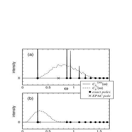
Figure 6: The Fourier transformed correlation functions, $C_{\beta}^{\rm CAN}(\omega)$ and $C_{\beta}^{c}(\omega)$: (a) for $\beta=1$ and (b) for $\beta=10$. The exact poles at $\omega=\omega_{m,n}$ and the EPAC pole at $\omega=\omega_{\beta}$ are also plotted.

As mentioned above, the EPAC is an approximation to extract the effective periodic oscillation from the exact correlation function. Therefore, it can be useful for the investigation of the systems where quantum coherence is significant. On the other hand, the CMD is a method to approximate the exact spectrum $C_{\beta}^{\rm CAN}(\omega)$ by a continuous spectrum, so that it is not proper to analyze the long time behavior of such systems. However, it has been found by Krilov and Berne, that the CMD gives much better results in a system under isobaric conditions, where the exact correlation function has a continuous spectrum kb . They also suggested that the CMD might give fairly accurate results in a dissipative system, because in such a system the quantum coherence is dephased through the interaction with the dissipative environment not to play an important role at longer time.

IV.3 Possible improvement

The EPAC method can be improved by means of the higher order derivative expansion of the effective action $\Gamma_{\beta}[Q]$. For example, the second order derivative expansion in Eq. (19) is

$$\Gamma_{\beta}[Q] = \int^{\beta\hbar}_{0}d\tau\left[V_{\beta}(Q)+\frac{1}{2}Z_{\beta}(Q)\dot{Q}^{2}\right].$$ (68)

Note the difference from Eq. (48). Then we obtain the correlation function as a result of the second-order EPAC  note ,

$$C^{{\rm AC}(2)}_{\beta}(t) = \left(\frac{\hbar}{2Z_{\beta}\omega_{\beta}^{S}}\coth\frac{\beta\hbar\omega_{\beta}^{S}}{2}\right)\cos\omega_{\beta}^{S}t-i\left(\frac{\hbar}{2Z_{\beta}\omega_{\beta}^{S}}\right)\sin\omega_{\beta}^{S}t+Q_{\rm min}^{2},$$ (69)

where $Z_{\beta}=Z_{\beta}(Q_{\rm min})$ and

$$\omega_{\beta}^{S} = \sqrt{\frac{1}{Z_{\beta}}\left.\frac{\partial^{2}V_{\beta}}{\partial Q^{2}}\right|}_{Q=Q_{\rm min}}.$$ (70)

The second-order EPAC correlation function again consists of a single oscillation mode, because the second-order derivative expansion only introduces the quantum/thermal correction to the particle mass, $m\to Z_{\beta}$, and never changes the number of the poles. In fact, it is expected that the $n(>2)$th order derivative expansion improves the qualitative behavior of the EPAC correlation functions by introducing additional poles. In such cases, the $n$th order EPAC correlation function $C_{\beta}^{{\rm AC}(n)}(t)$ would exhibit quasi-periodic oscillation more similar to the exact behavior.

Figure 7: The real parts of the quantum correlation functions at zero temperature: the exact quantum correlation function $C(t)$, the leading order EPAC correlation function $C^{\rm AC}(t)$, and the second-order EPAC correlation function $C^{{\rm AC}(2)}(t)$.

To see the effectiveness of this improvement, we now present a zero temperature example. At zero temperature, the exact real time quantum correlation function is

$$C(t) = \langle 0|~{}\!\hat{q}(t)\hat{q}(0)|0\rangle=\sum_{m}e^{-i(E_{m}-E_{0})t/\hbar}\left|\langle m|\hat{q}|0\rangle\right|^{2}.$$ (71)

On the other hand, the leading order EPAC correlation function is

$$C^{\rm AC}(t) = \frac{\hbar}{2m\omega_{\rm eff}}e^{-i\omega_{\rm eff}t}+Q^{2}_{\rm min},$$ (72)

where $\omega_{\rm eff}=\omega_{\beta}|_{\beta\to\infty}$, and the second order EPAC correlation function obtained from Eq. (69) is

$$C^{{\rm AC}(2)}(t) = \frac{\hbar}{2Z_{\rm eff}\omega_{\rm eff}^{S}}e^{-i\omega_{\rm eff}^{S}t}+Q^{2}_{\rm min},$$ (73)

where $Z_{\rm eff}=Z_{\beta}|_{\beta\to\infty}$ and $\omega_{\rm eff}^{S}=\omega_{\beta}^{S}|_{\beta\to\infty}$. To evaluate these zero temperature quantities, $\omega_{\rm eff}$, $Z_{\rm eff}$, and $\omega_{\rm eff}^{S}$, we employed the renormalization group technique wk for convenience; the effective frequency $\omega_{\rm eff}$ was calculated by solving the local potential approximated Wegner-Houghton equation wh ; nprg , while for $Z_{\rm eff}$ and $\omega_{\rm eff}^{S}$, we used the values obtained by solving the proper time renormalization group equation za . Figure 7 shows the real part of the exact quantum correlation function $C(t)$ and the real parts of the EPAC correlation functions: the leading order $C^{\rm AC}(t)$ and the second order $C^{{\rm AC}(2)}(t)$. It is seen that the deviation of the leading order EPAC correlation function $C^{\rm AC}(t)$ from the exact quantum correlation function is improved in the second-order EPAC ($C^{{\rm AC}(2)}(t)$), both in its initial ($t=0$) value and in its long time behavior.

The higher order derivative expansion is required especially for the analyses of many-body systems at higher temperature, because the multipole contribution to the correlation functions is significant for describing the decay of them. However, it is not easy to compute the higher derivative terms in $\Gamma_{\beta}$, especially at finite temperature. Therefore, it is a future task to establish an algorithm for computing them.

V CONCLUDING REMARKS

As a novel approximation method to evaluate the real time quantum correlation functions at finite temperature, we have newly proposed the EPAC method. The EPAC method has been tested in the one-dimensional symmetric double-well system, in comparison with another approximation scheme, the CMD method. The EPAC method and the CMD method are based on each different type of effective potential, the standard effective potential $V_{\beta}(Q)$ and the effective classical potential $V_{\beta}^{c}(q_{c})$, respectively. At first, we have evaluated $V_{\beta}^{c}(q_{c})$ by means of the normal mode PIMD calculation, and then $V_{\beta}(Q)$ have been obtained from it. It has been found that these effective potentials have the predicted formal properties: The equivalence of them in the zero temperature limit and the convexity of $V_{\beta}(Q)$. Then the real time two-point position correlation functions have been calculated by means of each approximation method. The CMD approximation is found to be good at short time range owing to its exactness at $t=0$, while at longer time it largely deviates from the exact correlation function because of the ensemble dephasing. On the other hand, our EPAC approximation can reproduce the long time oscillating behavior which originates from the quantum coherence of the system. Therefore, the EPAC should be very effective for the system in which quantum coherence is significant, such as the quantum double well system considered here. We have also suggested that the EPAC method can be improved by the higher order derivative expansion, and have shown, as an example, the result of the second order improvement at zero temperature. It has been seen that this improvement procedure works very well for this example.

In this paper we have restricted the arguments to the evaluation of the real time two-point position correlation function $C_{\beta}(t)=\langle\hat{q}(t)\hat{q}(0)\rangle_{\beta}$. Also for general correlation functions of nonlinear operators, e.g., $\langle\hat{q}^{n}(t)\hat{q}^{n}(0)\rangle_{\beta}$, the EPAC can be applied to evaluate them, because the $n$-point correlation function is obtained with the knowledge of the $n$th functional derivative of the effective action riv ; swa ; ps ; kl . This will be an interesting subject to be examined in near future.

As matters of theoretical interest, there are a number of subjects to be investigated. The role of the standard effective potential in the quantum transition-state theory gil ; vm should be clarified. Furthermore, it is interesting to find possible relationship between the effective potential-based methods of the present type and the other approaches to quantum dynamical correlations blt . It is worthwhile to pay attention to the fact that, for example, the effective potential-based quantum dynamics has been discussed in the context of the projection operator approach cgtv .

Finally we mention the direction of the applications of the EPAC to real molecular systems of chemical interest. From the results given in Sec. IV, it is suggested that the EPAC should be very effective for the systems where quantum coherence plays an important role. For example, proton transfer reactions proton are typical phenomena of such category, because the small mass of proton makes quantum coherence significant even at room temperature. The EPAC will properly represent the quantum oscillating behavior accompanied with proton transfers. For example, for a molecular reaction system where the intrinsic reaction coordinate (IRC) fukui is well-defined, once the IRC and the potential energy surface along it are provided, it is straightforward to calculate the approximate real time quantum correlation function by use of the EPAC method. However, for reactions occurring in solvents, not only the IRC but the full quantum calculations treating many degrees of freedom should be implemented. For the application of the EPAC to such many-body systems including quantum coherence, more efficient sampling algorithms or novel approximation schemes must be developed to calculate the effective classical potentials needed in the EPAC.

Appendix A ON THE RELATION BETWEEN $C^{c}_{\beta}(0)$ and $C^{\rm CAN}_{\beta}(0)$

It has been known that the CMD approximation [Eq. (32)] is exact at $t=0$, i.e., $C^{c}_{\beta}(0)=C^{\rm CAN}_{\beta}(0)$ jv ; rrjv ; ra . Note that this relation holds only for the correlation function of linear operator, as seen in the following simple derivation:

$$C_{\beta}^{\rm CAN}(0) = \frac{1}{\beta}\int_{0}^{\beta}d\lambda~{}\langle\hat{q}(-i\hbar\lambda)\hat{q}\rangle_{\beta}$$ (74)

$$= \frac{1}{\beta\hbar}\int_{0}^{\beta\hbar}du~{}\langle\hat{q}(-iu)\hat{q}\rangle_{\beta}$$

$$= \langle\hat{q}_{0}\hat{q}\rangle_{\beta}$$

$$= \langle\hat{q}_{0}~{}\!\frac{1}{\beta\hbar}\sum_{n=-\infty}^{\infty}\hat{q}(\omega_{n})\rangle_{\beta}$$

$$= \langle\hat{q}_{0}~{}\!\hat{q}_{0}\rangle_{\beta}$$

$$= \frac{1}{{\cal Z}_{\beta}}\int^{\infty}_{-\infty}dq\int^{q(\beta\hbar)=q}_{q(0)=q}{\cal D}q~{}\!q_{0}~{}\!q_{0}~{}\!e^{-S_{E}/\hbar}$$

$$= \frac{1}{{\cal Z}_{\beta}}\int^{\infty}_{-\infty}dq_{c}\int^{\infty}_{-\infty}dq\int^{q(\beta\hbar)=q}_{q(0)=q}{\cal D}q~{}\!q_{0}~{}\!q_{0}~{}\!\delta(q_{0}-q_{c})~{}\!e^{-S_{E}/\hbar}$$

$$= \frac{1}{{\cal Z}_{\beta}}\int^{\infty}_{-\infty}dq_{c}~{}\!q_{c}~{}\!q_{c}~{}\!\int^{\infty}_{-\infty}dq\int^{q(\beta\hbar)=q}_{q(0)=q}{\cal D}q~{}\!\delta(q_{0}-q_{c})~{}\!e^{-S_{E}/\hbar}$$

$$= \frac{1}{{\cal Z}_{\beta}}\int^{\infty}_{-\infty}dq_{c}~{}\!q_{c}~{}\!q_{c}~{}\!\rho_{\beta}^{c}(q_{c})$$

$$= \langle q_{c}~{}\!q_{c}\rangle_{\rho_{\beta}^{c}}$$

$$= C_{\beta}^{c}(0),$$

where we have used $q(\tau)=(1/\beta\hbar)\sum_{n=-\infty}^{\infty}e^{-i\omega_{n}\tau}q(\omega_{n})$,

$$\langle\hat{q}(-\omega_{n})~{}\!\hat{q}(\omega_{m})\rangle_{\beta} = \delta_{nm}\frac{\beta\hbar}{2}\int^{\beta\hbar}_{-\beta\hbar}due^{-i\omega_{n}u}\langle\hat{q}(u)~{}\!\hat{q}(0)\rangle_{\beta},$$ (75)

and the definition of path centroid $q_{0}=q(\omega_{0})/\beta\hbar$.

References

• (1) R. P. Feynman and A. R. Hibbs, Quantum Mechanics and Path integrals (McGraw-Hill, New York, 1965); R. P. Feynman, Statistical Mechanics (Addison-Wesley, New York, 1972).
• (2) B. J. Berne and D. Thirumalai, Ann. Rev. Phys. Chem. 37, 401 (1986), and references cited therein.
• (3) D. M. Ceperley, Rev. Mod. Phys. 67, 279 (1995), and references cited therein.
• (4) G. Baym and D. Mermin, J. Math. Phys. 2, 232 (1961).
• (5) A.A. Abrikosov, L.P.Gor’kov, and Dzyaloshinskii, Sov. Phys. JETP 36(9), 636 (1959); E.S. Fradkin, Sov. Phys. JETP 36(9), 912 (1959).
• (6) D. Thirumalai and B. J. Berne, J. Chem. Phys. 79, 5029 (1983).
• (7) N. Silver, J. E. Gubernatis, D. S. Sivia, and M. Jarrell, Phys. Rev. Lett. 65, 496 (1990); R. N. Silver, D. S. Sivia, and J. E. Gubernatis, Phys. Rev. B41, 2380 (1990); J. E. Gubernatis, M. Jarrell, R. N. Silver, and D. S. Sivia, ibid. 44, 6011 (1991).
• (8) E. Gallicchio and B. J. Berne, J. Chem. Phys. 101, 9909 (1994); 105, 7064 (1996); E. Gallicchio, S. A. Egorov, and B. J. Berne, ibid. 109, 7745 (1998).
• (9) Y. Nakahara, M. Asakawa, and T. Hatsuda, Phys. Rev. D60, 091503 (1999); Prog. Part. Nucl. Phys. 46, 459 (2001).
• (10) M. Topaler and N. Makri, J. Chem. Phys. 101, 7500 (1994).
• (11) C. H. Mak and R. Egger, J. Chem. Phys. 110, 12 (1999).
• (12) A. Sethia, S. Sanyal, and Y. Singh, J. Chem. Phys. 93, 7268 (1990); 96, 2428(E) (1992); A. Sethia, S. Sanyal, and F. Hirata, Chem. Phys. Lett. 315, 299 (1999); J. Chem. Phys. 114, 5097 (2001).
• (13) R. P. Feynman and H. Kleinert, Phys. Rev. A34, 5080 (1986).
• (14) R. Giachetti and V. Tognetti, Phys. Rev. Lett. 55, 912 (1985); Phys. Rev. B33, 7647 (1986).
• (15) J. Goldstone, A. Salam, and S. Weinberg, Phys. Rev. 127, 965 (1962); G. Jona-Lasinio, Nuovo Cim. 34, 1719 (1964).
• (16) P. M. Stevenson, Phys. Rev. D30, 1712 (1984); 32, 1389 (1985)
• (17) H. Verschelde, S. Schelstraete, J. Vandekerckhove, and J. L. Verschelde, J. Chem. Phys. 106, 1556 (1997); S. Schelstraete and H. Verschelde, J. Phys. Chem. A101, 3 (1997); J. Chem. Phys. 108, 7152 (1998).
• (18) A. Okopi$\grave{\rm n}$ska, Phys. Lett. A249, 259 (1998).
• (19) H. Jirari, H. Kröger, X. Q. Luo, K. J. M. Moriarty, and S. G. Rubin, Phys. Rev. Lett. 86, 187 (2001); Phys. Lett. A281, 1 (2001); L. A. Caron, H. Jirari, H. Kröger, X. Q. Luo, G. Melkonyan, and K. J. M. Moriarty, ibid. 288, 145 (2001); H. Jirari, H. Kröger, X. Q. Luo, G. Melkonyan, and K. J. M. Moriarty, ibid. 303, 299 (2002); H. Kröger, Phys. Rev. A65, 052118 (2002).
• (20) R. Fukuda and E. Kyriakopoulos, Nucl. Phys. B85, 354 (1975); R. Fukuda, Prog. Theor. Phys. 56, 258 (1976).
• (21) U. M. Heller and N. Seiberg, Phys. Rev. D27, 2980 (1983).
• (22) L. O’Raifeartaigh, A. Wipf, and H. Yoneyama, Nucl. Phys. B271, 653 (1986).
• (23) J. Kuti and Y. Shen, Phys. Rev. Lett. 60, 85 (1988).
• (24) A. Cuccoli, V. Tognetti, R. Vaia, and P. Verrucchi, Phys. Rev. A45, 8418 (1992); A. Cuccoli, V. Tognetti, P. Verrucchi, and R. Vaia, Phys. Rev. B46, 11601 (1992); Phys. Rev. Lett. 77, 3439 (1996); A. Cuccoli, R. Giachetti, V. Tognetti, R. Vaia, and P. Verrucchi, J. Phys. Cond. Matt. 7, 7891 (1995).
• (25) M. J. Gillan, J. Phys. C20, 3621 (1987).
• (26) G. A. Voth, D. Chandler, and W. H. Miller, J. Chem. Phys. 91, 7749 (1989); G. A. Voth, J. Phys. Chem. 97, 8365 (1993).
• (27) S. Coleman, Aspects of symmetry (Cambridge University Press, Cambridge, 1985).
• (28) J. Cao and G. A. Voth, J. Chem. Phys. 99, 10070 (1993); 100, 5093 (1994); 100, 5106 (1994); 101, 6168 (1994); 101, 6184 (1994); G. A. Voth, Adv. Chem. Phys. XCIII, 135 (1996).
• (29) R. Kubo, N. Toda, and N. Hashitsume, Statistical Physics II (Springer, Berlin, 1985).
• (30) S. Jang and G. A. Voth, J. Chem. Phys. 111, 2357 (1999); 111, 2371 (1999).
• (31) J. Cao and G. J. Martyna, J. Chem. Phys. 104, 2028 (1996); J. Cao, L. W. Ungar, and G. A. Voth, ibid. 104, 4189 (1996); J. Lobaugh and G. A. Voth, ibid. 104, 2056 (1996); 106, 2400 (1997); M. Pavese and G. A. Voth, Chem. Phys. Lett. 249, 231 (1996); A. Calhoun, M. Pavese, and G. A. Voth, ibid. 262, 415 (1996); K. Kinugawa, P. B. Moore, and M. L. Klein, J. Chem. Phys. 106, 1154 (1997); 109, 610 (1998); K. Kinugawa, Chem. Phys. Lett. 292, 454 (1998); S. Miura, S. Okazaki, and K. Kinugawa, J. Chem. Phys. 110, 4523 (1999); U. W. Schmitt and G. A. Voth, ibid. 111, 9361 (1999); S. Jang, Y. Pak, and G. A. Voth, J. Phys. Chem. A103, 10289 (1999); M. Pavese, S. Jang, and G. A. Voth, Parallel Computing 26, 1025 (2000); U. W. Schmitt and G. A. Voth, Chem. Phys. Lett. 329, 36 (2000); G. K. Schenter, B. C. Garett, and G. A. Voth, J. Chem. Phys. 133, 5171 (2000).
• (32) G. Krilov and B. J. Berne, J. Chem. Phys. 111, 9140 (1999); 111, 9147 (1999).
• (33) R. J. Rivers, Path Integral Methods in Quantum Field Theory (Cambridge University Press, Cambridge, 1987).
• (34) M. S. Swanson, Path Integrals and Quantum Processes (Academic, Boston, 1992).
• (35) M. E. Peskin and D. V. Schroeder, An Introduction to Quantum Field Theory (Addison-Wesley, New York and Tokyo, 1995).
• (36) H. Kleinert, Path Integrals in Quantum Mechanics Statistics and Polymer Physics (World Scientific, Singapore, 1995).
• (37) K. G. Wilson and J. B. Kogut, Phys. Rep. 12, 75 (1974).
• (38) F. Wegner and A. Houghton, Phys. Rev. A8, 401 (1973).
• (39) D. R. Reichman, P. -N. Roy, S. Jang, and G. A. Voth, J. Chem. Phys. 113, 919 (2000).
• (40) M. Le Bellac, Thermal Field Theory (Cambridge University Press, Cambridge, 1996).
• (41) It should be also noted that the correlation function $C_{\rm ref}(t)$ in the analytically continued effective harmonic theory is obtained from the superposition of the correlation functions for the effective harmonic oscillators defined at each centroid position $q_{c}$ with frequency $\bar{\omega}_{c}(q_{c})$. Each correlation function is then weighted by the centroid density $\rho_{\beta}^{c}(q_{c})$, and therefore $C_{\rm ref}(t)$ exhibits the ensemble dephasing like the CMD correlation function $C_{\beta}^{c}(t)$.
• (42) T. L. Curtright and C. B. Thorn, J. Math. Phys. 25, 541 (1984).
• (43) F. Cametti, G. Jona-Lasinio, C. Presilla, and F. Toninelli, Proceedings of the International School of Physics “Enrico Fermi,” Course CXLIII, edited by G. Casati, I. Guarneri, U. Smilansky (IOS Press, Amsterdam, 2000), p. 431.
• (44) R.Ramirez, T. Lopez-Ciudad, and J. C. Noya, Phys. Rev. Lett. 81, 3303 (1998); R.Ramirez and T. Lopez-Ciudad, J. Chem. Phys. 111, 3339 (1999).
• (45) G. Andronico, V. Branchina, and D. Zappala, Phys. Rev. Lett. 88, 178901 (2002); R.Ramirez, T. Lopez-Ciudad, and J. C. Noya, ibid. 88, 178902 (2002).
• (46) R. Jackiw and A. Kerman, Phys. Lett. A71, 158 (1979).
• (47) M. E. Tuckerman, D. Marx, M. L. Klein, and M. Parrinello, J. Chem. Phys. 104, 5579 (1996).
• (48) G. J. Martyna, M. L. Klein, and M. Tuckerman, J. Chem. Phys. 97, 2635 (1992).
• (49) K.-I. Aoki, A. Horikoshi, M. Taniguchi, and H. Terao, Prog. Theor. Phys. 108, 571 (2002); A. S. Kapoyannis and N. Tetradis, Phys. Lett. A276, 225 (2000).
• (50) D. Zappala, Phys. Lett. A290, 35 (2001).
• (51) For an asymmetric potential, $Q_{\rm min}$ has a finite value and the EPAC correlation function is shifted by a constant term $Q_{\rm min}^{2}$ according to Eq. (56).
• (52) Since we consider an approximation beyond the leading order, it could alternatively be called as the effective action analytic continuation (EAAC).
• (53) U. Balucani, M. H. Lee, and V. Tognetti, Phys. Rep. 373, 409 (2003), and references cited therein.
• (54) A. Cuccoli, R. Giachetti, V. Tognetti, and R. Vaia, J. Phys. A 31, L419 (1998)
• (55) Proton transfer in Hydrogen-Bonded Systems, edited by D. Bountis (Plenum, New York, 1992); Electron and Proton Transfer in Chemistry and Biology, edited by A. Müller, H. Ratajczak, W. Junge, and E. Diemann (Elsevier, Amsterdam, 1992).
• (56) K. Fukui, J. Phys. Chem. 74, 4161 (1970); K. Fukui, S. Kato, and H. Fujimoto, J. Am. Chem. Soc. 97, 1 (1975).