Theory of Plasmon-assisted Transmission of Entangled Photons

Abstract

The recent surface plasmon entanglement experiment [E. Altewischer et al., Nature (London) 418, 304 (2002)] is theoretically analyzed. The entanglement preservation upon transmission in the non-focused case is found to provide information about the interaction of the biphoton and the metallic film. The entanglement degradation in the focused case is explained in the framework of a fully multimode model. This phenomenon is a consequence of the polarization-selective filtering behavior of the metallic nanostructured film.

Entanglement Schrödinger (1935a, b, c) is one of the most strange properties of quantum mechanics. Despite its puzzling character, this property, which is directly linked to the non-local nature of the theory, has been tested many times. The first experiments were performed with simple systems comprising two photons Freedman and Clauser (1972); Aspect et al. (1982) or two atoms Hagley et al. (1997). Recently, entanglement has started to be considered as a resource for diverse applications in quantum information theory. This has driven the interest in the demonstration of entanglement for systems involving many particles. Large systems are more prone to decoherence processes and, therefore, entanglement should be a very fragile property for them. For this reason the experiment of Julsgaard et al. Julsgaard et al. (2001) showing entanglement between two gaseous caesium samples, and the plasmon-assisted transmission of entangled photons shown by Altewischer et al. Altewischer et al. (2002a) have both attracted quite a lot of interest. This Letter is devoted to Altewischer’s experience. Although some theoretical aspects of the experiment have been treated in the original paper and in Ref. Velsen et al. (2003), a general (multimode) theory is still lacking. Here a complete detailed theory is derived and a thorough analysis addressing all aspects of the experiment is presented.

In the experiment, pairs of correlated photons are generated by spontaneous parametric down conversion. The desired input polarization-entangled biphoton state is obtained by appropriate manipulation of the generated photon pairs Kwiat et al. (1995). This state is a quasi-monochromatic ($\lambda\simeq 813\,\textrm{nm}$) quasi-plane wave (propagating along the $Z$ axis) in the polarization singlet $(|X_{1}Y_{2}\rangle-|Y_{1}X_{2}\rangle)/\sqrt{2}$, where $X$ and $Y$ denote horizontal and vertical polarization, respectively, and the subscripts ($i=1,2$) label the first and second photon. After travelling along their respective trajectories parallel to the $Z$ axis, each photon traverses a polarizer $\textrm{P}_{i}$ and is measured by a detector $\textrm{D}_{i}$ [$\textrm{P}_{i}$ is orthogonal to the $Z$ axis and rotatable around it (the angle between the optic axis of $\textrm{P}_{i}$ and the $X$ axis will be denoted as $\beta_{i}$)]. These measured signals are electronically combined to obtain the rate of coincident photon detections. Such a setup allows one to determine the biphoton fringe visibility $V_{\beta_{2}}$ for fixed $\beta_{2}$, which is a measure of the photons entanglement degree Kwiat et al. (1995).

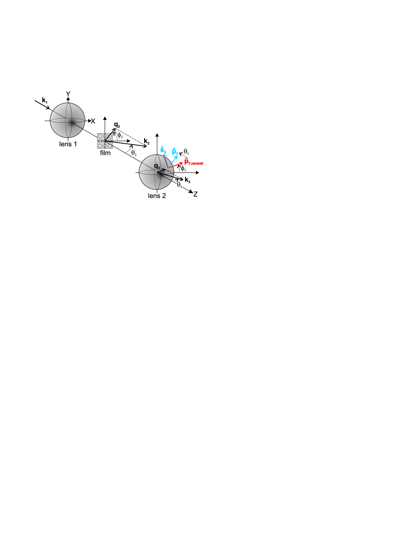
Figure 1: Optical elements in the trajectory of photon 1. The lenses, that constitute a confocal telescope, are only present in some parts of the experiment. The incident photon is represented by a monochromatic plane wave with wave vector $\textbf{k}_{1}=(\textbf{q}_{1},k_{1z})=(\textbf{0},k)$. The first lens produces a focused beam including many plane waves with wave vectors $\textbf{k}_{2}=(\textbf{q}_{2},k_{2z})$. The second lens gives rise again to a bundle of modes with $\textbf{k}_{3}=(\textbf{q}_{3},k_{3z})$. The unit vectors $\hat{\textbf{p}}_{3}$, $\hat{\textbf{s}}_{3}$ indicate the $p$ and $s$ polarization directions, respectively, whereas $\hat{\textbf{p}}_{3\,\textrm{paraxial}}=\hat{\textbf{q}}_{3}$.

Photon 2 propagates freely from the source to $\textrm{P}_{2}$, whereas photon 1 traverses a 200 nm thick Au film deposited on top of a 0.5 mm glass substrate (Fig. 1). The metallic film is drilled with cylindrical holes (200 nm diameter) arranged as a square lattice (period 700 nm). The transmission of photon 1 through the metallic film (at $\lambda\simeq 813\,\textrm{nm}$) is due to the phenomenon of extraordinary light transmission mediated by surface plasmon modes Ebbesen et al. (1998); Martín-Moreno et al. (2001). The chosen wavelength corresponds (almost) to a transmission resonance ascribed to a surface mode at the metal-glass interface and propagating along the diagonals of the hole array, i.e., a $(\pm 1,\pm 1)$ mode. In order to investigate the effect of focusing on the entanglement behavior upon transmission, the film is positioned at the focus of a confocal telescope in some parts of the experiment (lenses’ focal length $f=15\,\textrm{mm}$, telescope’s numerical aperture 0.13). Altewischer et al. report entanglement preservation upon transmission when no telescope is used. The entanglement is however degraded when photon 1 is focused on the hole array and, moreover, the measured visibilities $V_{0^{\circ}}$ and $V_{45^{\circ}}$ are different.

A careful interaction model of the biphoton with the hole array should explicitly include in the wave function the quantum state of the solid. In a simplified monomode case (i.e., without telescope), the initial wave function is $|\Phi_{\textrm{in}}\rangle=(|X_{1}Y_{2}\rangle-|Y_{1}X_{2}\rangle)/\sqrt{2}\otimes|S\rangle$, where $|S\rangle$ is the initial state of the solid. When the interaction has finished, the wave function $|\Phi_{\textrm{out}}\rangle$ can be written as:

$$t_{X_{1}X_{1}}|X_{1}Y_{2}\rangle\otimes|S_{xx}\rangle+t_{Y_{1}X_{1}}|Y_{1}Y_{2}\rangle\otimes|S_{yx}\rangle$$

$$- t_{X_{1}Y_{1}}|X_{1}X_{2}\rangle\otimes|S_{xy}\rangle-t_{Y_{1}Y_{1}}|Y_{1}X_{2}\rangle\otimes|S_{yy}\rangle,$$ (1)

where $t_{AB}$ are the transmission amplitudes for the various channels, and $|S_{ab}\rangle$ are normalized wave functions for the final state of the solid. The system’s final quantum state is defined by post-selection, and for this reason $|\Phi_{\textrm{out}}\rangle$ only includes terms with exactly two photons. In other words, processes where, for instance, photon 1 is absorbed do indeed exist ($t_{0X_{1}}|0Y_{2}\rangle\otimes|S_{0x}\rangle-t_{0Y_{1}}|0X_{2}\rangle\otimes|S_{0y}\rangle$), but they are not relevant for the visibility measurement because only coincident photons are registered. Notice that the final states of the solid must be taken into account, as may be clearly seen by considering the two following extreme situations: (i) all $|S_{ab}\rangle$ are orthogonal to each other. In this case the solid and the biphoton can be entangled to a larger or lesser extent (depending on the $t_{AB}$ values) but the biphoton state (obtained by tracing over the solid) is always a mixture of factorizable states and it is therefore completely disentangled Hill and Wootters (1997). Let us point out that in this case, after passage of photon 1, the solid incorporates a “which-polarization” information linked to the photons polarization state. This translates into an entanglement loss. (ii) all $|S_{ab}\rangle$ are equal. In this case the solid and the biphoton are completely disentangled, and the biphoton state can range from factorizable to maximally entangled depending on the $t_{AB}$ values. Since entanglement is preserved in some parts of Altewischer’s experiment, (ii) is our model for the interaction process, i.e., the interaction does not introduce “which-way” labels in the solid. Such a theoretical framework explains why entanglement is preserved when the photon 1 is not focused. It is a simple consequence of two facts: first, no “which-way” labels are introduced in the solid, and second, the transfer matrix $t_{AB}$ for an orthogonally incident plane wave (non-focused) on a square hole array is (by symmetry) proportional to the identity.

Within the present model the visibility computation only requires the determination of the transfer matrix $t_{AB}$ for the employed optical set up. When the telescope is used (to focus the field at a spot on the film), it is necessary to consider a multimode theory. The calculation proceeds as follows: (i) the electromagnetic field of photon 1 is expanded in plane waves $|\textbf{q}\,\,\sigma\rangle$ before and after each optical element ($\sigma=\{p,s\}$ denotes the two possible polarizations; see Fig. 1). (ii) Lens and film are described by their transfer matrices in the aforementioned basis, $\mathbb{L}(\textbf{q}_{2},\textbf{q}_{1})$, $\mathbb{F}(\textbf{q}_{2})$, respectively. (iii) These matrices are combined to obtain the transfer matrix $\mathbb{T}(\textbf{q}_{3},\textbf{q}_{1})$ of the telescope with the hole array inside it. (iv) The biphoton transfer matrix $\mathbb{M}(\textbf{q}_{3},\textbf{q}_{1})$ for the whole set up (including polarizers) is then given by the tensor product of the transfer matrices for each photon, i.e., $\mathbb{M}(\textbf{q}_{3},\textbf{q}_{1})=\mathbb{P}_{1}(\textbf{q}_{3})\mathbb{T}(\textbf{q}_{3},\textbf{q}_{1})\otimes\mathbb{P}_{2}(\textbf{0})$, where $\mathbb{P}_{i}$ are the polarizers’ transfer matrices. In the case of normal incidence, the telescope plus hole array transfer matrix $\mathbb{T}(\textbf{q}_{3},\textbf{0})$ turns out to be:

$$\mathbb{R}(\phi_{3})\int d\textbf{q}_{2}e^{i\frac{(n-1)\Delta}{2nk}(\textbf{q}_{2}-\frac{nf}{(n-1)\Delta}\textbf{q}_{3})^{2}}\mathbb{R}^{-1}(\phi_{2})\mathbb{F}(\textbf{q}_{2})\mathbb{R}(\phi_{2}),$$ (2)

where $\mathbb{R}$ is the two-dimensional rotation matrix, $n$ and $\Delta$ are the substrate refractive index and thickness, respectively ($n=1.52$), $k$ is the wave number, $f$ is the focal length, and the remaining variables are explained in Fig. 1. Note that the rapidly oscillating phase inside the integral means that the amplitude of $|\textbf{q}_{3}\rangle$ is mainly given by the $|\textbf{q}_{2}\rangle$ modes inside the telescope around the stationary phase condition $\textbf{q}_{2}=nf\textbf{q}_{3}/(n-1)\Delta$.

To obtain Eq. (2) a few approximations have been done. First, due to the low numerical aperture of the telescope, paraxial equations can be used. The lens transfer matrix $\mathbb{L}(\textbf{q}_{2},\textbf{q}_{1})$ is given by:

$$\frac{f}{2\pi ki}e^{i\frac{f}{2k}(\textbf{q}_{2}-\textbf{q}_{1})^{2}}\mathbb{R}(\phi_{2})\mathbb{R}^{-1}(\phi_{1}),$$ (3)

where the subscripts ($j=1,2$) refer to modes before and after the lens, respectively. Free propagation of a $|\textbf{q}_{2}\,\,\sigma_{2}\rangle$ mode inside the telescope along a distance $z$ amounts to an extra phase that, apart from global factors, is given by $\exp(-iz\textbf{q}_{2}^{2}/2k)$ in the paraxial approximation. Second, the detectors are located at the back focal plane of an auxiliary lens placed after the polarizers. This implies that each point in the detector essentially collects one $|\textbf{q}_{3}\rangle$ (in the limit of very large auxiliary lens aperture). For this reason the relative phases of the $|\textbf{q}_{3}\rangle$ modes after the telescope are not relevant for the visibility computation. Third, concerning the hole array, again due to the low numerical aperture of the telescope, it is enough to keep the 0-th diffracted order (higher orders are not collected by the second lens), and therefore the film transfer matrix $\mathbb{F}(\textbf{q})$ is q-diagonal. This matrix is numerically computed as explained in Martín-Moreno et al. (2001). Figure 2 shows the computed transmittance when the hole array is illuminated by an orthogonally incident (non-focused) plane wave, and the film is tilted around the diagonal (compare to Figs. 1b, 1c in Altewischer et al. (2002a)). Despite the simulations do not exactly give the experimental peaks’ heights and widths values, all main features are reproduced, including number and position of peaks, and overall order of magnitude. The behavior of the photonic bands as a function of parallel momentum is also correctly described.

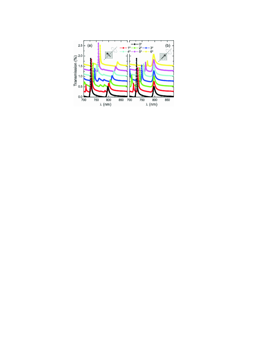
Figure 2: Hole array transmittance as a function of wavelength. The film is illuminated by an orthogonally incident plane wave (non-focused), and it is tilted (from $0^{\circ}$ to $6^{\circ}$) around the diagonal. The incident field linear polarization is perpendicular to the lattice diagonal in (a) and parallel to it in (b). For clarity the curves are offset 0.25%.

The transfer matrix $\mathbb{T}(\textbf{q}_{3},\textbf{0})$ corresponding to telescope plus film can be worked out analytically when $\textbf{q}_{3}=\textbf{0}$, i.e., when the detector’s aperture is extremely small. In this case the matrix before the integral in Eq. (2) disappears and the phase inside the integrand does not depend on $\phi_{2}$. If one writes down explicitly $\mathbb{T}(\textbf{0},\textbf{0})$ and takes into account the symmetry properties of the hole array, it can be shown that $\mathbb{T}(\textbf{0},\textbf{0})$ is proportional to the identity [note that this result does not depend on the particular model for the numerical computation of $\mathbb{F}(\textbf{q})$]. For this reason the whole set up should again preserve entanglement when only the following channels $(\textbf{q}_{1}=\textbf{0})\rightarrow(\textrm{all}\,\,\textbf{q}_{2})\rightarrow(\textbf{q}_{3}=\textbf{0})$ are considered. This means that the focusing of photon 1 does not by itself degrade entanglement in every situation but, rather, only when the transfer matrix $t_{AB}$ is not proportional to the identity. This could be easily checked in an experiment by inserting an iris before the detector.

Figure 3 shows the visibilities obtained when the telescope is again employed, but now all channels [$(\textbf{q}_{1}=\textbf{0})\rightarrow(\textrm{all}\,\,\textbf{q}_{2})\rightarrow(\textrm{all}\,\,\textbf{q}_{3})$] are considered. The visibility decreases as the telescope semiaperture increases (for $0^{\circ}$ semiaperture the monomode case is obviously recovered). The same behavior observed in Altewischer et al. (2002a) for the $(\pm 1,\pm 1)$ mode is reproduced by the simulations for $\lambda=797\,\textrm{nm}$ and telescope semiaperture $8^{\circ}$: $V_{45^{\circ}}=89\%$, $V_{0^{\circ}}=37\%$ (87 and 73 in the experiment, respectively). The numerical discrepancy for $V_{0^{\circ}}$ can be essentially attributed to the fact that the computed transmission resonances are narrower than the measured ones, and the visibility is very sensitive to this variable. It is also to be noted that in Altewischer et al. (2002a) the employed wavelength is a bit larger than the resonant wavelength whereas we have computed the visibility at the resonance maximum itself ($\lambda=797\,\textrm{nm}$). Our simulations show that $V_{0^{\circ}}$ grows for wavelengths larger than the resonant one ($V_{0^{\circ}}=52\%$ for $\lambda=802\,\textrm{nm}$), whereas $V_{45^{\circ}}$ remains approximately the same. Note that the visibilities are not monotone functions of the semiaperture. This is due to the fact that for larger semiapertures, higher values of $\theta_{2}$ are included in the integral of Eq. (2), and this permits the excitation of surface modes different from $(\pm 1,\pm 1)$ (as can be indirectly seen in Fig. 2).

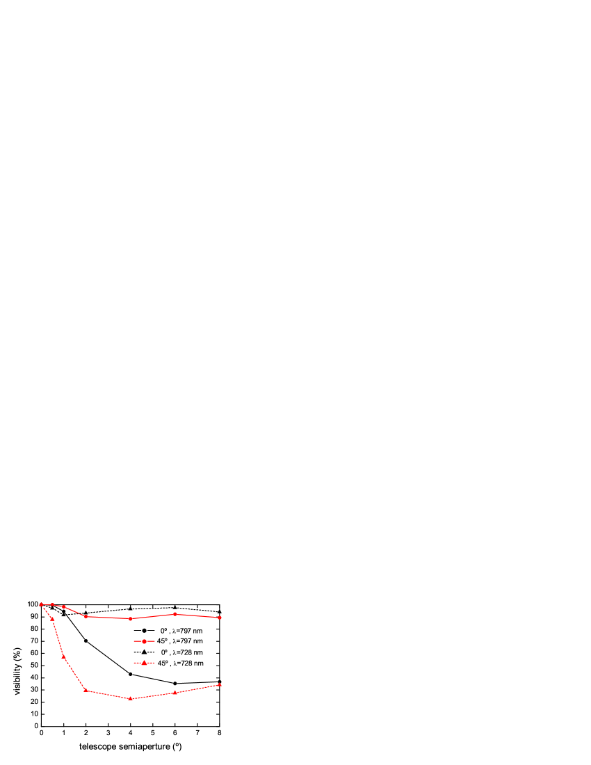
Figure 3: Biphoton fringe visibility as a function of the telescope semiaperture. The visibilities are shown for two orientations of the second polarizer: $\beta_{2}=0^{\circ},\,45^{\circ}$. The chosen wavelengths are the resonances shown in Fig. 2 for no tilt: 797 nm (corresponding to a surface mode propagating along the array diagonals), and 728 nm (corresponding to a mode propagating along the $X$ or $Y$ axes).

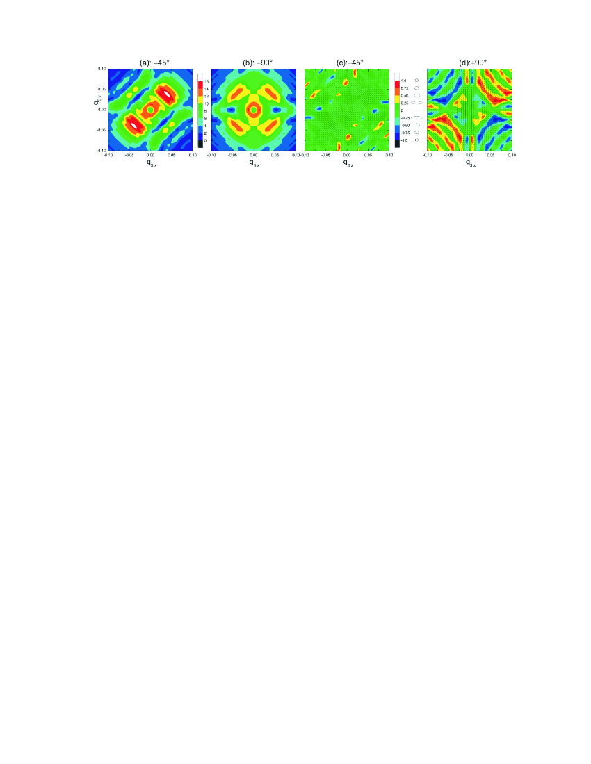
Figure 4: Intensities (a, b) and polarizations (c, d) of mode $|\textbf{q}_{3}\rangle$ after the telescope as a function of $(q_{3x},q_{3y})$. The excitation is one single linearly polarized photon ($\lambda=797\,\textrm{nm}$). The incident photon polarizations are $-45^{\circ}$ in (a, c) and $90^{\circ}$ in (b, d). The telescope semiaperture is $8^{\circ}$. The left color scale (arb. units) is shared by (a) and (b), and the right color scale corresponds to (c) and (d). In (c, d) the color scale represents the ratio of the minor to the major polarization elipse axes (for instance, $\pm 1$ correspond to left and right circular polarization), and the small line segments indicate the orientation of the elipse major axis. The maxima (and minima) of all abscissa and ordinate scales correspond to a semiaperture of $\theta_{3}=0.1^{\circ}$.

The visibility reduction (as compared to the non-focused case) can be understood because the transfer matrix $\mathbb{T}(\textbf{q}_{3},\textbf{0})$ of the telescope plus film is not proportional to the identity anymore. This means that the system acts as a polarization-selective filter. The initial balance between the $|X_{1}Y_{2}\rangle$ and $|Y_{1}X_{2}\rangle$ components (which is responsible of the maximal entanglement of the input state) is therefore destroyed and as a consequence the entanglement is degraded. In the following it will be explained why do $V_{45^{\circ}}$ and $V_{0^{\circ}}$ behave differently.

Let us remind that, when $V_{\beta_{2}}$ is measured, polarizer $\textrm{P}_{2}$ is set with this $\beta_{2}$. To understand the behavior of $V_{\beta_{2}}$ one can plot the field after the telescope due to a single photon 1 incident with $\beta_{2}\!+\!90^{\circ}$ linear polarization. This is so because the singlet biphoton state can be written as $(|\beta_{2}\,\,\beta_{2}\!+\!90^{\circ}\rangle-|\beta_{2}\!+\!90^{\circ}\,\,\beta_{2}\rangle)/\sqrt{2}$ for every $\beta_{2}$ (i.e., it is polarization isotropic). $V_{\beta_{2}}$ will be 100% if there exists an orientation $\beta_{1}$ for polarizer $\textrm{P}_{1}$ that completely blocks the field due to photon 1 incident with linear polarization $\beta_{2}\!+\!90^{\circ}$. Otherwise, as $\beta_{1}$ is varied, the collected intensity oscillates between a non-zero minimum and a maximum, and $V_{\beta_{2}}<100\%$. Such a polarization information is displayed in Fig. 4. Let us start with the analysis for $V_{45^{\circ}}$. For $-45^{\circ}$ incident polarization of photon 1, only the $(+1,-1)$ and $(-1,+1)$ modes are excited. The output field is predominantly linearly polarized along $-45^{\circ}$ [Fig. 4(c)], yielding high $V_{45^{\circ}}$ (a low photon coincidence rate will be registered for $\beta_{1}=+45^{\circ}$). On the other hand the analysis for $V_{0^{\circ}}$ goes as follows. For $90^{\circ}$ photon 1 incident polarization, all $(\pm 1,\pm 1)$ modes are excited, the output field is generally eliptically polarized [Fig. 4(d)], and it includes various polarization directions. This fact is responsible for the decrease in $V_{0^{\circ}}$ (no $\beta_{1}$ exists that nearly blocks the field). Note that the central region of both diagrams is linearly polarized along the incident polarization direction. This fits with the transfer matrix being approximately proportional to the identity (for this region) and with the 100% visibility expected for small detector aperture, as discussed previously. It is also to be noticed that Fig. 4 (a) and (b) compare well with Figs. 2b, and 2d in Altewischer et al. (2002b) [the stationary phase condition mentioned above maps the diagram’s side lengths shown here ($2\theta_{3}=0.2^{\circ}$) to the $2\theta_{2}=17.6^{\circ}$ value shown in Altewischer et al. (2002b); as opposed to Altewischer et al. (2002b), circular fringes do not appear in Fig. 4 (a) and (b) in the range shown because multiple interferences in the substrate were not included in the calculation]. The $\lambda=728\,\textrm{nm}$ surface mode propagates along the $(\pm 1,0)$ and $(0,\pm 1)$ directions and, as a consequence of previous discussion, the roles of $V_{45^{\circ}}$ and $V_{0^{\circ}}$ should be exchanged (this is indeed observed in the polarization diagrams for $\lambda=728\,\textrm{nm}$, not shown here for brevity). In fact, compared to $\lambda=797\,\textrm{nm}$, the high and low visibility values are now exchanged, as it is distinctly seen in Fig. 3, where $V_{45^{\circ}}$ is low and $V_{0^{\circ}}$ is high.

In conclusion, a detailed multimode theoretical analysis of Altewischer et al. experiment has been presented. Entanglement preservation in the monomode case implies a particular model for the hole array-biphoton interaction, namely, this interaction cannot introduce “which-way” labels in the metallic film. Our model also reproduces the measured results in the focused case. The entanglement degradation is understood as a consequence of the polarization-selective filtering behavior of the hole array for non-orthogonal incidence. A polarization analysis explains the different values of the $0^{\circ}$ and $45^{\circ}$ visibilities.

References

- Schrödinger (1935a) E. Schrödinger, Naturwissenschaften 23, 807 (1935a).
- Schrödinger (1935b) E. Schrödinger, Naturwissenschaften 23, 823 (1935b).
- Schrödinger (1935c) E. Schrödinger, Naturwissenschaften 23, 844 (1935c).
- Freedman and Clauser (1972) S. J. Freedman and J. F. Clauser, Phys. Rev. Lett. 28, 938 (1972).
- Aspect et al. (1982) A. Aspect, J. Dalibard, and G. Roger, Phys. Rev. Lett. 49, 1804 (1982).
- Hagley et al. (1997) E. Hagley et al., Phys. Rev. Lett. 79, 1 (1997).
- Julsgaard et al. (2001) B. Julsgaard, A. Kozhekin, and E. S. Polzik, Nature (London) 413, 400 (2001).
- Altewischer et al. (2002a) E. Altewischer, M. P. van Exter, and J. P. Woerdman, Nature (London) 418, 304 (2002a).
- Velsen et al. (2003) J. L. Velsen, J. Tworzydlo, and C. W. J. Beenakker, arXiv:quant-ph/0211103 (2003).
- Kwiat et al. (1995) P. G. Kwiat et al., Phys. Rev. Lett. 75, 4337 (1995).
- Ebbesen et al. (1998) T. W. Ebbesen et al., Nature (London) 391, 667 (1998).
- Martín-Moreno et al. (2001) L. Martín-Moreno et al., Phys. Rev. Lett. 86, 1114 (2001).
- Hill and Wootters (1997) S. Hill and W. K. Wootters, Phys. Rev. Lett. 78, 5022 (1997).
- Altewischer et al. (2002b) E. Altewischer, M. P. van Exter, and J. P. Woerdman, arXiv:physics.optics/0208033 (2002b).