Comparison of LOQC C-sign gates with ancilla inefficiency and an improvement to functionality under these conditions

Abstract

We compare three proposals for non-deterministic C-sign gates implemented using linear optics and conditional measurements with non-ideal ancilla mode production and detection. The simplified KLM gate [Ralph et al, Phys.Rev.A 65, 012314 (2001)] appears to be the most resilient under these conditions. We also find that the operation of this gate can be improved by adjusting the beamsplitter ratios to compensate to some extent for the effects of the imperfect ancilla.

I Introduction

Linear optics Quantum Computation (LOQC) kni00 offers an elegant way of implementing quantum gates on optical qubits using the inherent non-linearity of conditional measurements. This is achieved by introducing ancilla photons which interact with the linear circuit and are then detected. However, it has been shown that the accuracy of the gate operation is strongly dependent on the quality of the detectors used to detect the ancilla photons glancy .

Three distinct architectures have now been suggested for implementing the fundamental two qubit gate, the control-sign (C-sign) ral00 ; kni01 ; pit00 . It is natural to ask firstly whether all these architectures are equally sensitive to ancilla detector efficiency and secondly if it is possible to optimize gate operation to counter (to some extent) the effects of detector inefficiency. In this paper we address these questions and include in our analysis the converse issue of inefficiency in ancilla production.

We begin in section II by presenting our analysis technique. In section III we introduce the three versions of the C-sign gate and then present our comparative analysis. In section IV we discuss improvements to the least sensitive of these gates. We conclude in section V.

II Gate Analysis

In performing the analysis of the gates we consider ideal qubits sent into a non-deterministic LOQC gate consisting of a linear optical circuit interacting with prepared ancilla modes. The ancilla modes are then detected and the state at the output modes is kept if the measurement successfully matches the condition required for correct operation. It is assumed that mode matching errors and loss in the optical circuit can be neglected, but that inefficiency in the production and detection of the ancilla cannot be neglected. When the ancilla detection result indicates successful gate operation the output state is compared with the expected output via their fidelity

$$\mathinner{\langle{\Psi_{exp}|\rho_{out}|\Psi_{exp}}\rangle}$$

where $\rho_{out}$ is the output density operator and $\mathinner{|{\Psi_{exp}}\rangle}$ is the expected output. The fidelity is calculated in this way for all input states and the minimum fidelity is found. This is then taken as the figure of merit used for comparison. Under ideal conditions the fidelity is one for all inputs but lower numbers indicate reduced accuracy of the gate. Inefficient production and detection in ancilla modes are expected to have two effects: reduction in the probability of successful gate operation and a reduction in the fidelity when successful operation occurs.

Detector and input inefficiencies are simulated by introducing a beamsplitter with a reflectivity equal to the efficiency. The refected mode of each beamsplitter remains in the system and the transmitted mode is lost. No information can be retrieved in the loss mode so a partial trace is performed over this mode leaving the system in a mixed state.

For the sake of computational simplicity all the gates are analyzed in a single rail format lun00 , where the zero photon state $\mathinner{|{0}\rangle}$ represents logical zero and the single photon state $\mathinner{|{1}\rangle}$ represents logical one. In single rail format the C-sign operation is defined by:

$$\mathinner{|{0}\rangle}\mathinner{|{0}\rangle} \longrightarrow \mathinner{|{0}\rangle}\mathinner{|{0}\rangle}$$

$$\mathinner{|{0}\rangle}\mathinner{|{1}\rangle} \longrightarrow \mathinner{|{0}\rangle}\mathinner{|{1}\rangle}$$

$$\mathinner{|{1}\rangle}\mathinner{|{0}\rangle} \longrightarrow \mathinner{|{1}\rangle}\mathinner{|{0}\rangle}$$

$$\mathinner{|{1}\rangle}\mathinner{|{1}\rangle} \longrightarrow -\mathinner{|{1}\rangle}\mathinner{|{1}\rangle}$$

Single qubit manipulations are difficult using single rail logic. Thus dual rail logic mil88 is normally adopted in practice with the qubit defined across two optical modes. The logical zero is represented by a single photon occupation of one mode with the other in the vacuum state. The logical one is the reverse of the logical zero state with a single photon in the other mode. In LOQC, dual rail logic is often implemented using the horizontal and vertical polarization modes of a single spatial mode. For the special case of a C-sign gate the dual rail form is equivalent to the single rail form, just with added modes which do not participate in any interactions (see figure 1).

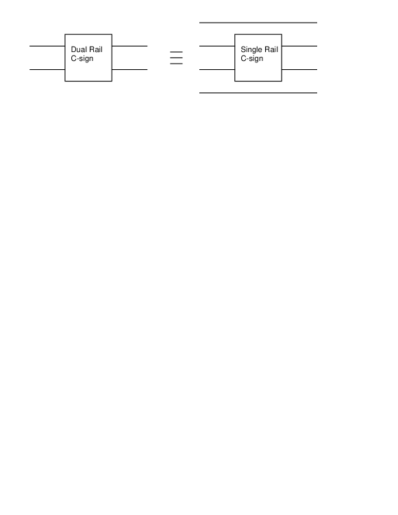
Figure 1: This diagram shows that the dual rail form is equivalent to the single rail form with extra modes. In dual rail format the lines represent two modes usually the horizontal and vertical modes of a single spatial mode. In the single rail format the lines represent one mode and the qubit is encoded in the photon number.

This can be seen from the definition of C-sign operation in the dual rail format (written in photon occupation form):

$$(\mathinner{|{1}\rangle}\mathinner{|{0}\rangle})(\mathinner{|{1}\rangle}\mathinner{|{0}\rangle}) \longrightarrow (\mathinner{|{1}\rangle}\mathinner{|{0}\rangle})(\mathinner{|{1}\rangle}\mathinner{|{0}\rangle})$$

$$(\mathinner{|{1}\rangle}\mathinner{|{0}\rangle})(\mathinner{|{0}\rangle}\mathinner{|{1}\rangle}) \longrightarrow (\mathinner{|{1}\rangle}\mathinner{|{0}\rangle})(\mathinner{|{0}\rangle}\mathinner{|{1}\rangle})$$

$$(\mathinner{|{0}\rangle}\mathinner{|{1}\rangle})(\mathinner{|{1}\rangle}\mathinner{|{0}\rangle}) \longrightarrow (\mathinner{|{0}\rangle}\mathinner{|{1}\rangle})(\mathinner{|{1}\rangle}\mathinner{|{0}\rangle})$$

$$(\mathinner{|{0}\rangle}\mathinner{|{1}\rangle})(\mathinner{|{0}\rangle}\mathinner{|{1}\rangle}) \longrightarrow -(\mathinner{|{0}\rangle}\mathinner{|{1}\rangle})(\mathinner{|{0}\rangle}\mathinner{|{1}\rangle}).$$

The first two bracketed states represent the first qubit while the second two represent the second qubit. Note that if the first mode is removed from all the qubits in the dual rail format then the single rail format is obtained. Because the extra modes do not participate in C-Sign gates (the assumed sources of loss are not present), single rail and dual rail fidelities are identical. Once in the dual rail format Control-NOT operation can be constructed by mixing the two target modes (the modes on which the controlled operation is to be applied) on a 50:50 beamsplitter before and after the C-sign operation.

The fidelity of each of the gates was calculated as follows. The operator evolution equations of each particular gate were calculated and inverted. The density operator for the required input state (including ancilla) was evolved using the solutions from the inverted equations. The loss modes are traced over, and detected modes are projected onto the required state. The remaining density operator $\hat{\rho}_{out}$ describes the output state which is now normalized to have $\textrm{Tr}(\hat{\rho}_{out})=1$. This renormalization is because we only wish to consider the accuracy of the gate assuming a successful detection event; the success rate is considered separately. The fidelity of the gate is calculated by finding the minimum of $\mathinner{\langle{\Psi_{exp}}|}\hat{\rho}_{out}\mathinner{|{\Psi_{exp}}\rangle}$ over all input states where $\mathinner{|{\Psi_{exp}}\rangle}$ is the expected output state from the used input state $\mathinner{|{\Psi_{in}}\rangle}$. The general input state $\mathinner{|{\Psi_{in}}\rangle}$ was written as follows:

$$\mathinner{|{\Psi_{in}}\rangle} = \cos{\alpha}\mathinner{|{00}\rangle}+\sin{\alpha}\cos{\beta}\mathinner{|{10}\rangle}+$$

$$\sin{\alpha}\sin{\beta}\cos{\gamma}\mathinner{|{01}\rangle}+\sin{\alpha}\sin{\beta}\sin{\gamma}\mathinner{|{11}\rangle}.$$

The advantage of writing the state in this form is that the optimization for finding the minimum fidelity can be performed over the variables $\alpha$, $\beta$ and $\gamma$ instead of a constrained optimization.

III Gate Comparisons

The three C-sign gates that were compared in our analysis are as follows:

KLM

The original non-deterministic C-sign gate introduced by Knill, Laflamme and Milburn kni00 is based on the operation of the so-called non-linear sign shift (NS) gate, which performs the transformation

$$\alpha\mathinner{|{0}\rangle}+\beta\mathinner{|{1}\rangle}+\gamma\mathinner{|{2}\rangle}\longrightarrow\alpha\mathinner{|{0}\rangle}+\beta\mathinner{|{1}\rangle}-\gamma\mathinner{|{2}\rangle}.$$ (2)

A simplification of the original design, shown in figure 2, was introduced by Ralph et. al. ral00 and is used in our calculations. Vacuum ($0$) and single ($1$) photon states are injected into the ancilla modes. The gate succeeds when the output ancilla are detected to be in the same state as was injected. C-sign operation is achieved by placing an NS gate in each arm of a balanced Mach Zehnder interferometer as shown in figure 3.

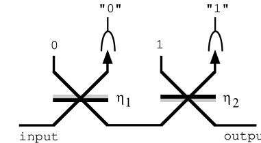
Figure 2: The non-deterministic gate which performs the operation described by equation 2. The beamsplitter reflectivities are $\eta_{1}=5-3\sqrt{2}$ and $\eta_{2}=(3-\sqrt{2})/7$.

Photon bunching in the interferometer then produces the sign shift when both control and target modes are in the $\mathinner{|{1}\rangle}$ state. The probability of success for the gate is approximately $1/20$.

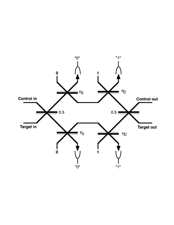
Figure 3: The (simplified) KLM control sign gate ral00 . The unnumbered beamsplitters have reflectivities $\eta_{1}=5-3\sqrt{2}$ and $\eta_{2}=(3-\sqrt{2})/7$.

Knill

Our second gate shown in figure 4 was introduced by Knill kni01 . It directly implements the C-sign operation. In contrast to the KLM gate it has no classical interferometric elements and requires only two ancilla, both prepared in single photon states. The gate succeeds when the output ancilla are both measured to be single photon states. The probability for success of the Knill gate is $1/13.5$.

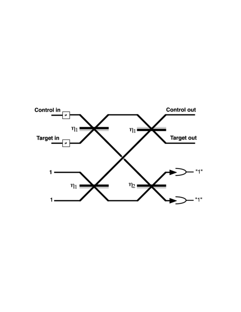
Figure 4: The knill control sign gate kni01 . The reflectivities are $\eta_{1}=\frac{1}{3}$ and $\eta_{2}=\frac{1}{6}(3+\sqrt{6})$. Note the beamsplitter convention here is different (see text).

PJF

Our third gate was introduced by Pittman, Jacobs and Franson  pit00 and is shown in figure 5. A related gate is that introduced by Koashi et. al. koashi . Unlike the other two gates, the PJF gate requires entanglement between the two ancilla modes. All beamsplitters have a reflectivity of 0.5. For the ancilla modes which are detected, the pairs of detectors shown must have exactly one photon, total, in the two modes for the gate to succeed. Rotations to the output may be necessary depending on which mode the single photon is found. The gate functionality is driven by the entanglement in the ancilla modes. The state of the four ancilla modes is (in the form $\mathinner{|{a_{1}a_{2}a_{3}a_{4}}\rangle}$) $(1/\sqrt{2})(\mathinner{|{0110}\rangle}+\mathinner{|{1001}\rangle})$. The probability of success of the PJF gate is $1/4$.

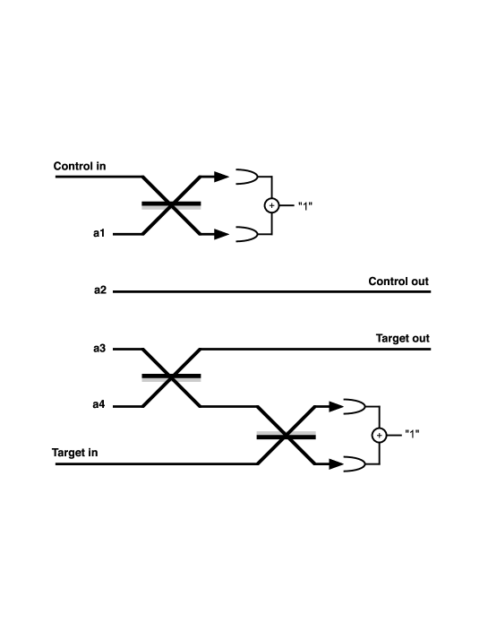
Figure 5: The Pittman, et. al. C-sign gate pit00 . The schematic here uses normal beamsplitters with reflectivities of $0.5$. The detector pairs must measure one photon in total. The ancilla modes are prepared as $\mathinner{|{a_{1}a_{2}a_{3}a_{4}}\rangle}\rightarrow(1/\sqrt{2})(\mathinner{|{0110}\rangle}+\mathinner{|{1001}\rangle})$

Throughout the remainder of this paper, the gates will be called by the names just introduced. Note that the beamsplitter conventions differ between the proposals. The KLM and PJF gates have beamsplitters which have a sign change on reflection off the grey side but the Knill gate has a sign change on transmission for beams incident on the black side.

Figure 6 shows the results of the fidelity calculations (as described in the previous section) for the three gates when only the detectors exhibit loss (i.e. perfect state input). The parameter along the abscissa is the detector efficiency and the ordinate shows the fidelity of the gate at that efficiency. The solid line represents the PJF gate, the dashed line shows the Knill gate and the dot-dashed line shows the KLM gate.

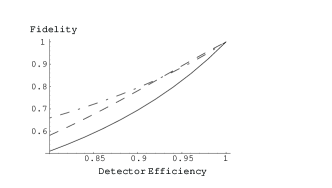
Figure 6: A comparison of the minimum fidelity of the three gates (PJF - solid, Knill - dashed, KLM - dot-dashed) as a function of the detector efficiencies.

All gates show a quite steep decrease in minimum fidelity as a function of efficiency, illustrating the sensitivity of LOQC gates to this sort of loss (recall though that this is minimum fidelity and so represents a worst case scenario). For detector efficiencies greater than about 93% the Knill gate gives marginally better performance, but for detector efficiencies below this value the KLM gate shows a better fidelity by a significant margin.

A similar analysis can be done with ancilla production efficiencies. Figure 7 shows this analysis and has the same gate - plot style correspondence as in figure 6. Once again a steep decrease in minimum fidelity as a function of efficiency is observed.

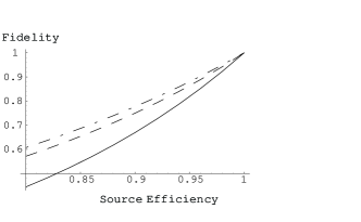
Figure 7: A comparison of the minimum fidelity of the three gates (PJF - solid, Knill - dashed, KLM - dot-dashed) as a function of the input efficiencies.

In this figure it can be seen that the KLM gate has the highest minimum fidelity for the range of efficiencies shown. From the figures we may conclude that, as assessed by minimum fidelity, the simplified KLM gate is in general the most forgiving in the presence of ancilla production and detection inefficiencies.

IV Gate Fidelity Improvement

One effect of reduced ancilla efficiency is to bias the probability of successful gate operation for different input states. This is a detrimental effect as some information about the input state is thus leaked through the statistics of the projective measurements success. In turn this results in biasing of the fidelities of the gate for different inputs. For example with the KLM gate the fidelity for the $\mathinner{|{0}\rangle}\mathinner{|{0}\rangle}$ input state is unaffected by ancilla inefficiencies while the $\mathinner{|{0}\rangle}\mathinner{|{1}\rangle}$ and $\mathinner{|{1}\rangle}\mathinner{|{0}\rangle}$ states are most strongly affected, with these states giving the minimum fidelity for this gate. This suggests it may be possible to improve upon the fidelity gained here if one were to adjust the elements in the gate to compensate for the biasing of gate functionality incurred due to the ancilla inefficiencies. Using this idea as a guide we have improved the performance of the KLM gate.

The KLM gate is constructed from two NS gates, which ideally perform the operation given in equation 2. The gate has two parameters which can be altered: the reflectivities of each of the two beamsplitters. Using the same technique as above for calculating the gate fidelity, we can optimize the fidelity with respect to these beamsplitter ratios for fixed detector and input efficiency. It is assumed that the two NS gates in the whole C-sign gate have the same beamsplitter ratios, maintaining the symmetry of the gate.

Figure 8 shows the fidelity of the simplified KLM gate when the prepared ancilla are kept the same and the detection scheme is the same as proposed, but the beamsplitter ratios in the two NS gates are varied. The ‘$\Delta\eta 1$’ and ‘$\Delta\eta 2$’ axes show the change in the beamsplitter ratios from their initial values; that is, for the point (0,0) the beamsplitter ratios have not changed. The z-axis shows the fidelity of the gate. The assumed loss with this diagram is 90% detector efficiency and perfect input efficiency.

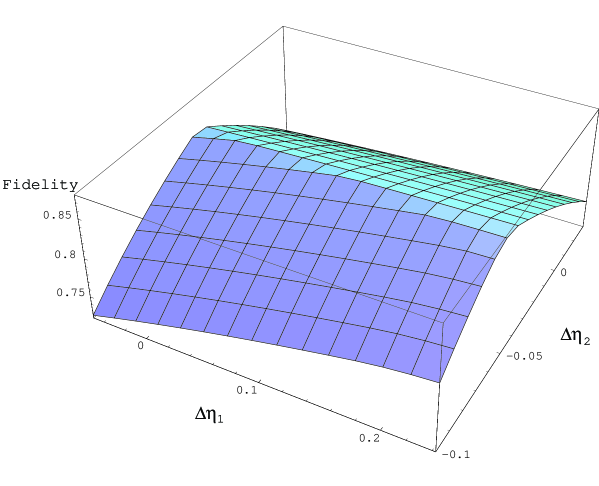
Figure 8: This plot shows the minimum fidelity (z-axis) of the modified KLM gate with detector efficiency of 0.9 and perfect ancilla input for a range of beamsplitter ratios of the two NS gates (x-y axes). The x-y axes show the change in the reflectivity from the normal reflectivities of the NS gate. The important feature of this plot is the increasing fidelity as $\eta_{1}$ is increased. The most positive value of $\eta_{1}$ shown here is the maximum value it can take.

The important feature of this plot is the increase of fidelity with $\eta_{1}$. To the far right of the $\eta_{1}$ axis is the limit of the allowed values for $\eta_{1}$. This limit is imposed by the necessity that reflectivities lie between zero and one. So in this case, the fidelity can be optimized by choosing the first beamsplitter perfectly reflective. Doing this, in effect, removes the detector which measures zero photons and removes the vacuum input. Inefficient equipment is removed from the gate and the gate complexity is reduced. All that remains is to optimize the fidelity along the ‘$\Delta\eta 2$’ axis. This feature of increasing fidelity with $\eta_{1}$ is seen here with detector efficiencies up to about 99%.

The increasing fidelity with $\eta_{1}$ is not seen with a lossy source. However, when the source efficiency drops slightly below unity the relationship between the gate fidelity and $\eta_{1}$ is almost flat. For source efficiency of about 98%, the improvement in the fidelity is only about $0.01$ at the actual optimized value of $\eta_{1}$ and $\eta_{2}$ compared with setting $\eta_{1}=1$. So for simplicity, the fidelity will be considered optimized at $\eta_{1}=1$ for both lossy sources and detectors.

Figure 9 shows the gate fidelity (optimized) with $\eta_{1}=1$ and $\eta_{2}$ at the optimum value. The graphs on the left show the fidelity without any alterations to the beamsplitters (solid line and) the optimized fidelity (dashed line). The plots on the right show what the $\eta_{2}$ value is for this optimized fidelity. There are three cases shown in figure 9. The first is perfect source efficiency and variable detector efficiency. The second is perfect detectors and variable source efficiency. The last is variable source and detectors but both have equal efficiencies.

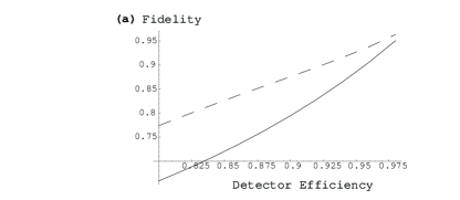
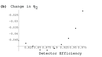
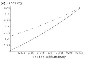
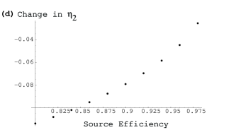
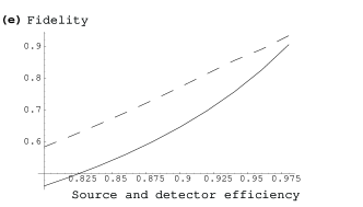
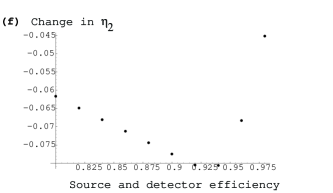
Figure 9: The graphs in this figure show many cases in which the fidelity of the modified KLM gate can be improved. The top row shows a simulation with detector efficiency considered only. The graph on the left shows the fidelity of the gate without any adjustments with the solid line. The dashed line in this plot shows the fidelity reached when optimized against $\eta_{2}$ ($\eta_{1}=1$). The amount that $\eta_{2}$ is changed by is shown in the plot on the right. This data is plotted with the detector efficiency along the abscissa. The other two sets of graphs show the same for source efficiency and finally detector and source efficiency both present but equal.

As an example of the small difference between using $\eta_{1}=1$ and varying it for non-unity source efficiency, the fidelity shown here for perfect detectors at 98% source efficiency is 0.956. When both $\eta_{1}$ and $\eta_{2}$ are varied a fidelity of 0.959 can be reached using $\eta_{1}=0.7703$ and $\eta_{2}=0.1838$. When a source efficiency of 0.8 is used, the fidelity reported here is 0.723 and a slight improvement (in the fourth decimal place) can be achieved at the values $\eta_{1}=0.9720$ and $\eta_{2}=0.1123$.

Figure 10 shows similar evidence that $\eta_{1}$ should be set to unity for all but the highest efficiencies. The figure is a zoomed region of the plots from figure 9 where detector and source efficiencies are equal and higher than 0.99.

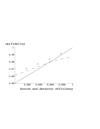
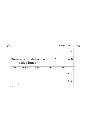
Figure 10: These plots are of the same form as those in figure 9. They are a zoomed region of the detector and source losses considered (but equal) near unity efficiency. This shows that setting $\eta_{1}=1$ can lead to an improvement until an efficiency of about 99.5% is reached. The dots shown on the left plot are the optimized fidelities when both $\eta_{1}$ and $\eta_{2}$ are varied.

Note from these figures that there is an improvement in fidelity with $\eta_{1}=1$ until efficiencies reach about 99.5%. Once again a slight improvement in these figures can be gained by varying $\eta_{1}$ (which is possibly the origin of the slight downwards bending of the improved fidelity curve).

Changing the parameters of the gate will change the probability that the gate will function successfully as shown in figure 11 for the case where detector and source losses are equal. The probability of the gate functioning does not drop below about $\frac{1}{5}$ the original value for detector and input efficiencies above about 0.8.

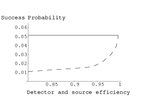
Figure 11: This plot shows the probability of success of the KLM gate when at the optimized value for $\eta_{2}$ and setting $\eta_{1}=1$. The case considered here is when detector and source losses are present and equal in magnitude. The solid line shows the probability of success of the gate with the beamsplitter ratios set to the usual values and with no losses.

This technique of tuning gate parameters to counter the effects of ancilla inefficiency could also be applied to the Knill and PJF gates in some form. However, it is not so clear how to proceed for these gates and it could be a computationally expensive task. Since the KLM gate gave the most encouraging results in the default setup and its parameter space is relatively small, its optimization was pursued here.

V Conclusion

Three LOQC C-sign gates have been compared using the minimum fidelity over all possible input states as the figure of merit. The KLM gate appears to be the most resilient to photon loss in ancilla detection for efficiencies below 95% and input loss for all efficiencies. The gate fidelity for the KLM gate can be improved by adjusting the beamsplitter ratios of the gate. In all but the most efficient conditions (loss less than 0.5%), it is best to remove the first beamsplitter from each of the two NS gates that make up the C-sign gate and adjust the second until optimum fidelity is reached. This actually reduces the complexity of the gate considerably by removing two photon counters. The improvement in minimum fidelity can be quite significant. Single photon production and detection efficiencies around 90% are not unreasonable in the short term. Under such conditions the optimized KLM gate could be expected to give fidelities $\geq 0.8$ for all operations, assuming all other imperfections can be neglected.

- (1) E. Knill, R. Laflamme and G. Milburn, Nature 409, 46, (2001).
- (2) S. Glancy, J. M. LoSecco, H. M. Vasconcelos, and C. E. Tanner Phys. Rev. A65, 062317 (2002)
- (3) T. C. Ralph, A. G. White, W. J. Munro and G. J. Milburn, Phys. Rev. A, 65, 012314 (2001).
- (4) E. Knill, Phys. Rev. A66, 052306 (2002).
- (5) T. B. Pittman, B. C. Jacobs, and J. D. Franson, Phys. Rev. A, 64, 062311 (2001).
- (6) A. P. Lund and T. C. Ralph, Phys. Rev. A, 66, 032307 (2002).
- (7) G. J. Milburn, Phys. Rev. Lett. 62, 2124 (1988).
- (8) M. Koashi, T. Yamamoto and N. Imoto Phys. Rev. A63 030301 (2001).