Controlling dipole-dipole frequency shifts in a lattice-based optical atomic clock

Abstract

Motivated by the ideas of using cold alkaline earth atoms trapped in an optical lattice for realization of optical atomic clocks, we investigate theoretically the perturbative effects of atom-atom interactions on a clock transition frequency. These interactions are mediated by the dipole fields associated with the optically excited atoms. We predict resonance-like features in the frequency shifts when constructive interference among atomic dipoles occur. We theoretically demonstrate that by fine-tuning the coherent dipole-dipole couplings in appropriately designed lattice geometries, the undesirable frequency shifts can be greatly suppressed.

I Introduction

The development of increasingly accurate atomic clocks has led to many advances in technology and tests of fundamental physics. In the search for the next generation of clocks and frequency standards, there has been considerable interest in using alkaline earth species because of their narrow intercombination lines in the optical spectrum hall89 . In order to achieve a high level of short-term stability and long-term reproducibility and accuracy on the clock transition, it is desirable to have a large number of cold atoms located in a well-characterized trap for an improved signal-to-noise ratio ($S/N$) and reduced systematic errors associated with atomic motion. Single ion-based systems do effectively eliminate Doppler and other motion-related systematic errors when the single ions are confined in the Lamb-Dicke regime rafac00 , although the achievable $S/N$ is limited by single quantum absorbers. For neutral atoms it is important that changes in the level structure due to the trapping potential do not alter the relevant clock transition frequency. Such a scheme has been proposed by trapping alkaline earth atoms in three-dimensional optical lattices tuned to a “magic” wavelength where the relevant states for the clock transition experience exactly the same level shift katori02 . The ${}^{1}S_{0}(F=9/2)-{}^{3}P_{0}(F=9/2)$ forbidden transition ($\lambda_{0}=700$ nm) in ⁸⁷Sr katori02 is in particular a promising candidate for a lattice-based optical clock transition because of the long lifetime of the excited state (${\sim}160$ s) and the insensitivity of the $J=0$ states to the polarization state of the trapping light. Already there have been efforts towards the cooling and trapping of ⁸⁷Sr mukaiyama03 ; xu03 ; xu03josab , and recently this transition was directly observed and measured for the first time courtillot03 . Calcium, another alkaline earth atom that has been studied extensively as a frequency standard Udem01 ; Wilpers02 , may be a candidate for optical lattice clocks as well.

In the case of $N$ independent atoms, one benefits from a $\sqrt{N}$ improvement in $S/N$ in spectroscopy. However, atoms trapped in an optical lattice can interact with each other and cannot truly be considered independent. Each optically excited atom represents essentially a point dipole whose radiated electromagnetic field can affect other atoms. These atom-atom interactions can manifest themselves as shifts in the observed transition frequencies. Because of the spatial ordering of atoms in a lattice and the potentially high atomic density, it is possible that such interactions may produce very large frequency shifts. One might expect then that dipole-dipole interactions can be much more severe here than in, for example, atomic fountains, and thus could place serious limits on the accuracy of an optical lattice clock if not accounted for. On the other hand, it might be possible to design lattice geometries where this shift is reduced or cancelled. Although the trapping lasers are constrained to operate at the “magic” wavelength, the lattice geometry can be altered by changing the relative orientations of the trapping beams, whose degrees of freedom can be characterized by a set of variables $\{\alpha\}$.

In this paper, we investigate theoretically the dipole-dipole interaction-induced shifts in the clock transition frequency recovered by Ramsey spectroscopy. We show that by varying the lattice geometry we can quantitatively control the clock frequency shift and even reduce the shift to zero. In particular, we give an analytical equation that can be solved giving configurations $\{\alpha_{0}\}$ where constructive interference causes the line shift to be very large. In these “bad” lattice configurations, the magnitude of the line shift scales approximately like $N^{2/3}$. Quite generally we propose that by tuning the parameter space $\{\alpha\}$ to lie in between two of these bad configurations, one can find “good” configurations where the shift is cancelled. The mechanism of cancellation is associated with the destructive interference of contributions to the shift from different atoms in the lattice.

It is important to emphasize that the present mechanism and theoretical treatment differ considerably from the conventional approaches used to treat dipole-dipole line broadening and shifts. In the case of atoms in a spatially-ordered lattice geometry, long-range effects are important, and the usual methods involving binary collisions of nearest neighbors allard82 are not applicable. These long-range effects include, in particular, interference of the far-field dipole radiation produced by the excited atoms, a phenomenon similar to Bragg scattering in a crystal.

This paper is organized as follows. In Sec. II we derive equations describing the evolution of an atomic system with dipole-dipole interactions. These equations are derived assuming that the atoms are in the Lamb-Dicke regime, with one atom or less per lattice site. In Sec. III we give a brief review of Ramsey spectroscopy and solve for the dipole-dipole induced line shift using perturbation theory. We find that the shift can be qualitatively understood in terms of the classical interaction energies between oscillating dipoles. There is a contribution to the shift that is zeroth order in the interrogation time $t$, which is due to imperfections in the Ramsey pulses. Even with perfect pulses, however, one finds a shift that is first order in $t$ that results from spontaneous decay of the atoms. Sec. IV discusses how our result for the line shift can be generalized for systems with imperfect filling of the lattice sites and for multilevel atoms. In the case of imperfect filling, one can calculate the mean value of the frequency shift as well as some nonzero variance, due to the uncertainty of how the lattice is filled. In Sec. V, we derive an equation that can be solved giving lattice configurations where the shift is large due to constructive interference. We derive an approximate scaling law for the shift in these “bad” configurations and discuss how the line shift can be reduced by choosing an appropriate lattice design. In Sec. VI we demonstrate these results numerically for one specific lattice configuration.

II Equations of motion

To treat the problem of interacting atoms in a lattice, we consider $N$ two-level atoms in the Lamb-Dicke limit with polarizability along the $z$-axis. A simple model of the system consists of treating the atoms as point dipoles, and we further assume that there is one or less atom per lattice site. This corresponds to a Mott-insulator state for bosons or a normal state for fermions. In principle, to solve exactly the problem of interacting atoms one would start from the full atom-field Hamiltonian and take into account not only all the atomic degrees of freedom but the continuum of electromagnetic field modes. To simplify the theoretical treatment, we effectively eliminate the field in the standard way using the Born-Markov approximation (see Appendix). This is valid provided that the atomic system evolves slowly on timescales of the correlation time $\tau_{c}$, which is of the order $L/c$ where $L$ is the linear size of the system and $c$ is the speed of light. As a result of eliminating the field, one finds an effective equation of motion for the density matrix $\rho$ of the atomic system. Atom-atom interactions then appear through an effective Hamiltonian $H_{\scriptsize{\textrm{eff}}}$ as well as through a non-Hermitian operator $\mathcal{L}$:

$$\frac{\partial\rho}{{\partial}t}=\frac{1}{i\hbar}\left[H_{0}+H_{\scriptsize{\textrm{eff}}},\rho\right]+\mathcal{L}[\rho].$$ (1)

Here, $H_{0}$ is the atomic Hamiltonian for a non-interacting system. Writing out all the terms in detail,

$$\frac{\partial\rho}{{\partial}t} = \frac{1}{i}\sum_{a}\left[\frac{\omega_{0}}{2}\sigma_{a}^{z},\rho\right]-\frac{i\Gamma}{2}\sum_{a{\neq}b}g(k\mathbf{r}_{ab})\left[\sigma_{a}^{+}\sigma_{b}^{-},\rho\right]$$ (2)

$$-\frac{\Gamma}{2}\sum_{a,b}f(k\mathbf{r}_{ab})\left(\left\{\sigma_{a}^{+}\sigma_{b}^{-},\rho\right\}-2\sigma_{b}^{-}\rho\sigma_{a}^{+}\right)-\frac{1}{4}\sum_{a}\gamma\left(\rho-\sigma_{a}^{z}\rho\sigma_{a}^{z}\right),$$

where

$$f(\mathbf{v}) = \frac{3}{2}\left(\sin^{2}\theta\frac{\sin{v}}{v}+(3\cos^{2}\theta-1)\left(\frac{\sin{v}}{v^{3}}-\frac{\cos{v}}{v^{2}}\right)\right),$$

$$g(\mathbf{v}) = -\frac{3}{2}\left(\sin^{2}\theta\frac{\cos{v}}{v}+(3\cos^{2}\theta-1)\left(\frac{\cos{v}}{v^{3}}+\frac{\sin{v}}{v^{2}}\right)\right),$$ (3)

and $\theta$ is the angle that $\mathbf{v}$ makes with the $z$-axis.

The first term on the right-hand side of Eq. (2) corresponds to $H_{0}$. $\sigma_{a}^{z}$ is the Pauli matrix of atom $a$ corresponding to the population difference between the excited and ground states, and $\omega_{0}$ is the resonance frequency of the dipole transition. The second term corresponds to $H_{\scriptsize{\textrm{eff}}}$. Here, $\Gamma=k_{0}^{3}d^{2}/3\pi\epsilon_{0}\hbar$ is the spontaneous decay rate of the excited state of a single, isolated atom, where $k_{0}=2\pi/\lambda_{0}=\omega_{0}/c$ and $d$ is the dipole matrix element between the ground and excited states. $\sigma_{a}^{+}$ is the atomic raising operator on atom $a$, and $\sigma_{b}^{-}$ is the lowering operator on atom $b$. One then sees that the effect of dipole-dipole interactions is an exchange of excitation between pairs of atoms. The strength of interaction is modified by a function $g(k\mathbf{r}_{ab})$ that depends on the distance and orientation between two dipoles. It is to be understood that $k=k_{0}$ in the functions $f$ and $g$. We see that both short-range, near-field $(1/r^{3})$ and long-range, far-field $(1/r)$ dipole interactions are included in our formalism and are treated on equal footing. The third term on the right side of Eq. (2) corresponds to $\mathcal{L}$ and also is due to atom-atom interactions. It also depends on $\Gamma$ and has a position dependence described by $f(k\mathbf{r}_{ab})$. The non-Hermitian nature of this term is evident through the anticommutator. Physically $\mathcal{L}$ describes the processes of both independent and cooperative decay. Finally, we have also added phenomenological dephasing through the $\gamma$ term, which in particular includes the effects of a finite, short-term linewidth of the laser interrogating the clock transition.

From Eq. (2), one can derive equations of motion for any atomic operators. For our particular application of Ramsey spectroscopy, we find it necessary to solve for the coherence ${\langle}\sigma_{a}^{+}{\rangle}$ and the two-atom correlation ${\langle}\sigma_{a}^{z}\sigma_{b}^{+}{\rangle}$. Furthermore, to remove the rapid oscillations due to $\omega_{0}$, it is convenient to work in the frame rotating with the interrogating laser frequency $\omega_{L}$, where

$$\frac{\partial{\langle}\sigma_{a}^{+}{\rangle}}{{\partial}t} = -i\delta{\langle}\sigma_{a}^{+}{\rangle}-\frac{\Gamma+\gamma}{2}{\langle}\sigma_{a}^{+}{\rangle}+\frac{\Gamma}{2}\sum_{b{\neq}a}\left(f(k\mathbf{r}_{ab})-ig(k\mathbf{r}_{ab})\right){\langle}\sigma_{a}^{z}\sigma_{b}^{+}{\rangle},$$ (4)

$$\frac{\partial{\langle}\sigma_{a}^{z}\sigma_{b}^{+}{\rangle}}{{\partial}t} = -\left(i\delta+\frac{3\Gamma+\gamma}{2}\right){\langle}\sigma_{a}^{z}\sigma_{b}^{+}{\rangle}-\Gamma{\langle}\sigma_{b}^{+}{\rangle}-\frac{\Gamma}{2}\left(f(k\mathbf{r}_{ab})+ig(k\mathbf{r}_{ab})\right){\langle}\sigma_{a}^{+}{\rangle}-{\Gamma}f(k\mathbf{r}_{ab}){\langle}\sigma_{a}^{+}\sigma_{b}^{z}{\rangle}$$ (5)

$$+\frac{\Gamma}{2}\sum_{j{\neq}a,b}\left(f(k\mathbf{r}_{bj})-ig(k\mathbf{r}_{bj})\right){\langle}\sigma_{a}^{z}\sigma_{b}^{z}\sigma_{j}^{+}{\rangle}-\Gamma\sum_{j{\neq}a,b}\left(f(k\mathbf{r}_{aj})+ig(k\mathbf{r}_{aj})\right){\langle}\sigma_{a}^{+}\sigma_{b}^{+}\sigma_{j}^{-}{\rangle}$$

$$-\Gamma\sum_{j{\neq}a,b}\left(f(k\mathbf{r}_{aj})-ig(k\mathbf{r}_{aj})\right){\langle}\sigma_{a}^{-}\sigma_{b}^{+}\sigma_{j}^{+}{\rangle},$$

and $\delta=\omega_{L}-\omega_{0}$.

In principle, to solve for the atomic system exactly, equations of motion for higher-order correlations are needed, although typically some approximation is used to truncate the resulting hierarchy of equations. In general these equations can describe light-matter interactions in an optically dense medium, including radiation trapping, level shifts, and superradiance fleischhauer99 .

III Ramsey spectroscopy in optical lattice clock

III.1 Basic principles

We now analyze the effects of atom-atom interactions on Ramsey spectroscopy. Starting from the ground state $\mbox{$|g\rangle$}^{{\otimes}N}$ of the system, suppose that one applies a strong probe pulse with the interrogating laser, given in the rotating frame by the Hamiltonian

$$H=\sum_{a}i\hbar\Omega\left({\sigma_{a}^{+}}e^{i\mathbf{k}{\cdot}\mathbf{r}_{a}}-{\sigma_{a}^{-}}e^{-i\mathbf{k}{\cdot}\mathbf{r}_{a}}\right),$$ (6)

where $\Omega$ is the Rabi frequency. For simplicity, we have made a plane-wave assumption about the probing laser, taking $\mathbf{k}$ to be in the positive $x$ direction. We also assume that $k{\approx}k_{0}$, and suppress the subscript in future calculations. We can do this if the phase error $e^{i{\delta}L/c}$ over the length of the sample incurred by making this assumption is small. Applying this pulse for a time $\tau$ evolves the system through the unitary operator

$$U={\prod_{a}}^{\otimes}\left(\begin{array}[]{cc}\cos\Omega\tau&e^{ikx_{a}}\sin\Omega\tau\\ -e^{-ikx_{a}}\sin\Omega\tau&\cos\Omega\tau\end{array}\right).$$ (7)

The state vector immediately following this pulse is given by

$$\mbox{$|\psi_{i}\rangle$}={\prod_{a}}^{\otimes}\left(\cos\Omega\tau\mbox{$|g\rangle$}+e^{ikx_{a}}\sin\Omega\tau\mbox{$|e\rangle$}\right),$$ (8)

where $|e\rangle$ denotes the excited state of the clock transition.

In Ramsey spectroscopy, one lets $|\psi_{i}\rangle$ evolve for an interrogation time $t$ to $\rho(t)$. During this time the coherence between the ground and excited states acquires some time-dependent phase that depends on $\delta$. After a time $t$, one then applies a second pulse corresponding to the inverse unitary operation $U^{\dagger}$, and then measures the signal corresponding to $\tilde{S}=\sum_{a}\sigma_{a}^{z}$, averaged over the final system $\rho_{f}$. $\tilde{S}$ corresponds to the total population inversion. Because of the second pulse, $\tilde{S}$ will now depend on $\delta$ and $t$, allowing one to extract information about the resonance line.

Formally, we can rewrite $\tilde{S}$ as

$$\tilde{S} = \textrm{Tr}\left(\sum_{a}{\sigma_{a}^{z}}U^{\dagger}\rho(t)U\right)$$ (9)

$$= \cos{2\Omega\tau}{\langle}\sum_{a}\sigma_{a}^{z}{\rangle}-2\sin{2\Omega\tau}\textrm{Re}{\langle}\sum_{a}e^{ikx_{a}}\sigma_{a}^{+}{\rangle},$$

where the averages denoted above apply to $\rho(t)$, the system immediately before the second pulse.

In the case of $N$ non-interacting, independently decaying atoms,

$${\langle}\sigma_{a}^{z}{\rangle} = -1+e^{-{\Gamma}t}\left(1-\cos{2\Omega\tau}\right),$$ (10)

$${\langle}e^{ikx_{a}}\sigma_{a}^{+}{\rangle} = \frac{1}{2}\sin{2\Omega\tau}e^{-(i\delta+\Gamma/2+\gamma/2)t},$$ (11)

which gives a corresponding signal

$$\tilde{S}=-N\left(\cos{2\Omega\tau}\left(1-e^{-{\Gamma}t}\right)+e^{-{\Gamma}t}\cos^{2}{2\Omega\tau}+e^{-({\Gamma}+\gamma)t/2}\sin^{2}{2\Omega\tau}\cos{{\delta}t}\right).$$ (12)

One can see that there is a peak in the signal around $\delta=0$. Determination of this peak allows one to find the frequency of the transition. One can note two important points about $\tilde{S}$. The contrast in $\tilde{S}$ with respect to $\delta$ is maximized when a “perfect” $\pi/2$ pulse is applied, i.e., when $\Omega\tau=\pi/4$. Furthermore, the contribution to $\tilde{S}$ due to ${\langle}\sigma_{a}^{z}{\rangle}$ in Eq. (9) is independent of $\delta$ and thus plays no role in determination of the resonance line. Thus, one is motivated to define an effective signal $S$ that consists of the part of $\tilde{S}$ that is actually used to determine the line:

$$S=-2\sin{2\Omega\tau}\textrm{Re}{\langle}\sum_{a}e^{ikx_{a}}\sigma_{a}^{+}{\rangle}.$$ (13)

The equation above states that from a theoretical standpoint, determination of the resonance line by measuring the population inversion after the second Ramsey pulse is equivalent to measuring the real part of ${\langle}e^{ikx_{a}}\sigma_{a}^{+}{\rangle}$ directly before the second pulse.

III.2 Effect of interactions

Solving for $S$ exactly in the presence of dipole-dipole interactions appears to be quite a difficult task. Since all interactions are proportional to $\Gamma$, our approach is to solve for $S$ as a perturbative expansion in ${\Gamma}$. In particular, we solve for the coherence ${\langle}\sigma_{a}^{+}{\rangle}$ in Eq. (4) to second order in $\Gamma$. This requires solving ${\langle}\sigma_{a}^{z}\sigma_{b}^{+}{\rangle}$ in Eq. (5) to first order in $\Gamma$. The solution for the coherence with appropriate initial conditions is

$${\langle}\sigma_{a}^{+}{\rangle} = \frac{1}{2}e^{-ikx_{a}}\sin(2\Omega\tau)e^{-\left(i\delta+\gamma/2\right)t}\left[1-\frac{{\Gamma}t}{2}(1+C_{a})+\frac{({\Gamma}t)^{2}}{8}(1+C_{a})\right.$$ (14)

$$+\left.\frac{\Gamma^{2}}{2\gamma^{2}}\sum_{b{\neq}a}\left(f(k\mathbf{r}_{ab})-ig(k\mathbf{r}_{ab})\right)\left(A_{ab}\gamma^{2}t^{2}-2B_{ab}\left(e^{-{\gamma}t}+{\gamma}t-1\right)\right)\right],$$

where

$$A_{ab} = -\frac{3}{4}e^{ik(x_{a}-x_{b})}\cos(2\Omega\tau)+\frac{1}{2}e^{ik(x_{a}-x_{b})}+\frac{1}{4}\left(f(k\mathbf{r}_{ab})+ig(k\mathbf{r}_{ab})\right)-\frac{1}{2}f(k\mathbf{r}_{ab})\cos(2\Omega\tau)$$ (15)

$$-\frac{1}{4}\sum_{j{\neq}a,b}\left(f(k\mathbf{r}_{bj})-ig(k\mathbf{r}_{bj})\right)e^{ik(x_{a}-x_{j})}\cos^{2}(2\Omega\tau),$$

$$B_{ab} = \frac{1}{4}e^{ik(x_{a}-x_{b})}\sin^{2}(2\Omega\tau)\sum_{j{\neq}a,b}\left(f(k\mathbf{r}_{aj})\cos{kx_{aj}}+g(k\mathbf{r}_{aj})\sin{kx_{aj}}\right),$$ (16)

$$C_{a} = \sum_{b{\neq}a}\left(f(k\mathbf{r}_{ab})-ig(k\mathbf{r}_{ab})\right)e^{ik(x_{a}-x_{b})}\cos{2\Omega\tau}.$$ (17)

Eq. (14) is correct to every order of $\gamma$. Eqs. (13) and (14) can be evaluated numerically for a given lattice configuration and number of atoms. To illustrate the general features of the shift, however, we now make the following simplifications. We expand Eq. (14) to lowest order in $\gamma$. We also assume that the Ramsey pulses are nearly perfect $\pi/2$ pulses, i.e., $\cos{2\Omega\tau}=\epsilon{\ll}1$. We then keep terms like $\epsilon{\Gamma}t$ but ignore terms like $\epsilon\Gamma^{2}t^{2}.$ With these simplifications,

$${\langle}\sigma_{a}^{+}{\rangle}{\approx}\frac{1}{2}e^{-ikx_{a}}\sin(2\Omega\tau)e^{-i{\delta}t}\left(1-\frac{{\Gamma}t}{2}+\frac{({\Gamma}t)^{2}}{8}-\phi_{a}\right),$$ (18)

where

$$\phi_{a} = \sum_{b{\neq}a}\left(f(k\mathbf{r}_{ab})-ig(k\mathbf{r}_{ab})\right)e^{ik(x_{a}-x_{b})}\left(\frac{{\Gamma}t}{2}\cos(2\Omega\tau)+\frac{({\Gamma}t)^{2}}{4}\left(1+\frac{1}{2}\left(f(k\mathbf{r}_{ab})+ig(k\mathbf{r}_{ab})\right)e^{-ik(x_{a}-x_{b})}\right.\right.$$ (19)

$$+\left.\left.\frac{1}{2}\sum_{j{\neq}a,b}\left(f(k\mathbf{r}_{aj})\cos{kx_{aj}}+g(k\mathbf{r}_{aj})\sin{kx_{aj}}\right)\right)\right)$$

The first three terms in the parentheses of Eq. (18) are a result of expanding the $e^{-{\Gamma}t/2}$ term that appears in the result for independent atoms, given in Eq. (12). This is just the decay of the signal one would get from independent spontaneous emission. The last term in the parentheses is a correction due to atom-atom interactions. Plugging this result into Eq. (13), we find that

$$S{\approx}-\sin^{2}{2\Omega\tau}\left((\cos{\delta}t)\left(N-\frac{N{\Gamma}t}{2}+\frac{N({\Gamma}t)^{2}}{8}-\sum_{a}\textrm{Re}\phi_{a}\right)-(\sin{\delta}t)\sum_{a}\textrm{Im}\phi_{a}\right).$$ (20)

Because of the antisymmetric $\sin{\delta}t$ term now appearing in $S$, one immediately sees that dipole-dipole interactions introduce a shift $\delta_{p}$ in the Ramsey fringes, which can be found by solving ${\partial}S/{\partial}\delta=0$. Suppose that the inequalities $\delta_{p}t{\ll}1,{\Gamma}t{\ll}1$ are satisfied. Under these conditions, a simple expression for $\delta_{p}$ results:

$$\frac{\delta_{p}}{\Gamma} \approx \frac{1}{N}\sum_{a}\sum_{b{\neq}a}\left(g(k\mathbf{r}_{ab})\cos{kx_{ab}}-f(k\mathbf{r}_{ab})\sin{kx_{ab}}\right)\times$$ (21)

$$\left(\frac{1}{2}\cos{2\Omega\tau}+\frac{{\Gamma}t}{4}\left(1+\frac{1}{2}\sum_{j{\neq}a,b}\left(f(k\mathbf{r}_{aj})\cos{kx_{aj}}+g(k\mathbf{r}_{aj})\sin{kx_{aj}}\right)\right)\right).$$

III.3 Interpretation of shift

The shift given by Eq. (21) yields a simple interpretation. In anticipation of future analysis, we write $\delta_{p}$ as

$$\frac{\delta_{p}}{\Gamma}=\frac{1}{N}\sum_{a}\sum_{b{\neq}a}\tilde{U}_{ab}\times\left(\frac{1}{2}\epsilon+\frac{{\Gamma}t}{4}\tilde{\Gamma}_{a}\right),$$ (22)

where

$$\tilde{U}_{ab} = g(k\mathbf{r}_{ab})\cos{kx_{ab}}-f(k\mathbf{r}_{ab})\sin{kx_{ab}},$$ (23)

$$\epsilon = \cos{2\Omega\tau},$$ (24)

$$\tilde{\Gamma}_{a} = 1+\frac{1}{2}\sum_{j{\neq}a,b}\left(f(k\mathbf{r}_{aj})\cos{kx_{aj}}+g(k\mathbf{r}_{aj})\sin{kx_{aj}}\right).$$ (25)

We will see that $\tilde{U}_{ab}$ is a dimensionless quantity corresponding to the classical interaction energy between two oscillating dipoles, $\epsilon$ is a parameter characterizing the error in the Ramsey pulses, and $\tilde{\Gamma}_{a}$ is a dimensionless quantity characterizing cooperative decay of the system.

To show the meaning of the $\tilde{U}_{ab}$ term in Eq. (22), consider the interaction between a classical, oscillating dipole at $\mathbf{r}_{a}$ excited with phase $e^{i(kx_{a}-{\omega}t)}$ and the field incident on it due to a classical, oscillating dipole at $\mathbf{r}_{b}$ excited with phase $e^{i(kx_{b}-{\omega}t)}$. We assume that both dipoles are oriented along the $z$-axis and that their magnitudes $d$ are determined from the relation $\Gamma=k_{0}^{3}d^{2}/3\pi\epsilon_{0}\hbar$. The classical interaction energy between dipole $a$ and the incident field is given by $U_{ab}=-(1/2)\textrm{Re}(\mathbf{d}_{a}{\cdot}\mathbf{E}^{*}_{b}(\mathbf{r}_{a}))$. The field at $\mathbf{r}_{a}$ due to dipole $b$ is jackson99 :

$$E_{z}(\mathbf{r}_{a})=e^{i(kx_{b}-{\omega}t)}\frac{k^{3}d}{4\pi\epsilon_{0}}e^{ikr}\left(\frac{\sin^{2}\theta}{kr}+(3\cos^{2}\theta-1)\left(\frac{1}{(kr)^{3}}-\frac{i}{(kr)^{2}}\right)\right),$$ (26)

where $r=|\mathbf{r}_{b}-\mathbf{r}_{a}|$. Now using the definitions in Eq. (3), the interaction energy can readily be rewritten as:

$$U_{ab} = -\frac{1}{2}\textrm{Re}(\mathbf{d}_{a}\cdot\mathbf{E}_{b}^{*}(\mathbf{r}_{a}))=\frac{\hbar\Gamma}{4}\left(g(k\mathbf{r}_{ab})\cos{kx_{ab}}-f(k\mathbf{r}_{ab})\sin{kx_{ab}}\right)$$ (27)

$$= \frac{\hbar\Gamma}{4}\tilde{U}_{ab}.$$ (28)

One then sees that this indeed corresponds to the first term of Eq. (22).

Although the $\tilde{U}_{ab}$ term in Eq. (22) resembles a classical interaction energy, the terms in parentheses reflect the quantum mechanical nature of the system. There is a contribution to the shift that is zeroth order in the interrogation time $t$ and proportional to $\epsilon$. One notes that for perfect $\pi/2$ Ramsey pulses, $\epsilon=0$. Thus, the zeroth order shift is due to error in the Ramsey pulse. This can be understood by considering Eq. (4). One sees that the interaction terms only influence evolution of the coherence through the term ${\langle}\sigma_{a}^{z}\sigma_{b}^{+}{\rangle}$. For a perfect $\pi/2$ pulse, this term is initially zero, and in this case, interactions cannot affect the measurement at short times. This effect is due to the nature of dipole-dipole interactions: these interactions cannot influence the coherence ${\langle}\sigma_{a}^{+}{\rangle}$ of an atom when it is in an equal superposition of the ground and excited states.

Even if a perfect $\pi/2$ pulse is applied, there is an additional contribution to the shift that is first order in $t$ and whose strength is given by $\tilde{\Gamma}_{a}$. The intuition behind this is also straightforward. Even if ${\langle}\sigma_{a}^{z}\sigma_{b}^{+}{\rangle}$ is initially zero, decay of the excited state will eventually evolve ${\langle}\sigma_{a}^{z}{\rangle}$ away from zero and back towards its equilibrium value of $-1$. Once ${\langle}\sigma_{a}^{z}\sigma_{b}^{+}{\rangle}$ is nonzero, interactions can influence evolution of ${\langle}\sigma_{a}^{+}{\rangle}$. The rate of decay is characterized by $\tilde{\Gamma}_{a}$. The first term in $\tilde{\Gamma}_{a}$ is the contribution from independent decay of the atom back to the ground state. The second contribution involves a sum over other atoms and represents a correction due to the fact that the decay process may in fact be cooperative (e.g., superradiance). One can easily verify that the contribution from atom $j$ is proportional to $\textrm{Im}(\mathbf{d}_{a}\cdot\mathbf{E}_{j}^{*}(\mathbf{r}_{a}))$:

$$\textrm{Im}(\mathbf{d}_{a}\cdot\mathbf{E}_{j}^{*}(\mathbf{r}_{a})){\propto}f(k\mathbf{r}_{aj})\cos(kx_{aj})+g(k\mathbf{r}_{aj})\sin(kx_{aj}).$$ (29)

This reflects the well-known result that the atomic inversion ${\langle}\sigma_{a}^{z}{\rangle}$ is driven by the dipole component in quadrature with the incident field.

IV Generalization of results

IV.1 Imperfect filling of lattice sites

Experimentally, knowing the exact number of atoms in the lattice and achieving a filling factor of one atom per lattice site are difficult tasks. Most likely, one can experimentally determine the density $\rho(\mathbf{r})$ of atoms in the lattice, such that the probability of occupation at any particular site $a$ is $P(\mathbf{r}_{a})=\rho(\mathbf{r}_{a})V$, where $V$ is the volume of a unit cell. It is straightforward to modify Eq. (21) to the case of imperfect filling. For simplicity, we only consider the shift that is zeroth order in $t$. This shift can be written

$$\frac{\delta_{p}}{\Gamma} = \frac{1}{N}\sum_{a}\sum_{b{\neq}a}\frac{1}{2}\cos{2\Omega\tau}\left(g(k\mathbf{r}_{ab})\cos{kx_{ab}}-f(k\mathbf{r}_{ab})\sin{kx_{ab}}\right)$$ (30)

$$= \frac{2}{N}\sum_{\scriptsize{\textrm{pairs}}}\frac{1}{2}\cos{2\Omega\tau}\;g(k\mathbf{r}_{ab})\cos{kx_{ab}}$$ (31)

$$= \frac{1}{2}\cos{2\Omega\tau}\sum_{\mathbf{R}{\neq}0}U(\mathbf{R})\frac{N(\mathbf{R})}{N},$$ (32)

where $U(\mathbf{R})=g(k\mathbf{R})\cos{kR_{x}}$, $\{\mathbf{R}\}$ denotes the set of direct lattice vectors, and $N(\mathbf{R})$ is the number of pairs of atoms separated by $\mathbf{R}$. In the derivation above we have utilized the fact that $\sin{kx_{ab}}=-\sin{kx_{ba}}$ to cancel the sum of $f(k\mathbf{r}_{ab})\sin{kx_{ab}}$. In a realistic scenario, one neither knows $N(\mathbf{R})$ nor $N$ exactly. In this case, one must solve instead for the ensemble average ${\langle}\delta_{p}{\rangle}$ and the variance $\Delta\delta_{p}$. For large $N$, one can safely pull the factor of $N$ out of the ensemble average:

$${\langle}\frac{N(\mathbf{R})}{N}{\rangle}\approx\frac{{\langle}N(\mathbf{R}){\rangle}}{{\langle}N{\rangle}}.$$ (33)

With this simplification,

$$\frac{{\langle}\delta_{p}{\rangle}}{\Gamma} = \frac{1}{2{\langle}N{\rangle}}\cos{2\Omega\tau}\sum_{\mathbf{R}{\neq}0}U(\mathbf{R}){\langle}N(\mathbf{R}){\rangle}$$ (34)

$$= \frac{1}{2{\langle}N{\rangle}}\cos{2\Omega\tau}\sum_{\mathbf{R}{\neq}0}U(\mathbf{R}){\int}d\mathbf{r}\rho(\mathbf{r})\rho(\mathbf{r}+\mathbf{R})V,$$ (35)

$$\frac{(\Delta\delta_{p})^{2}}{\Gamma^{2}} = \left(\frac{1}{2{\langle}N{\rangle}}\cos{2\Omega\tau}\right)^{2}\sum_{\mathbf{R},\mathbf{R^{\prime}}{\neq}0}U(\mathbf{R})U(\mathbf{R}^{\prime}){\langle}N(\mathbf{R})N(\mathbf{R}^{\prime}){\rangle}$$ (37)

$$-\left(\frac{1}{2{\langle}N{\rangle}}\cos{2\Omega\tau}\sum_{\mathbf{R}{\neq}0}U(\mathbf{R}){\langle}N(\mathbf{R}){\rangle}\right)^{2}$$

$$= \left(\frac{1}{2{\langle}N{\rangle}}\cos{2\Omega\tau}\right)^{2}\left[\sum_{\mathbf{R},\mathbf{R^{\prime}}{\neq}0}U(\mathbf{R})U(\mathbf{R}^{\prime})\int{d}\mathbf{r}\rho(\mathbf{r})\rho(\mathbf{r}+\mathbf{R})V^{2}\Big{(}(1-\rho(\mathbf{r})V)\rho(\mathbf{r}+\mathbf{R^{\prime}})\right.$$

$$+\left.(1-\rho(\mathbf{r}+\mathbf{R})V)\rho(\mathbf{r}+\mathbf{R}+\mathbf{R^{\prime}})\right.+\left.(1-\rho(\mathbf{r})V)\rho(\mathbf{r}-\mathbf{R^{\prime}})\right.$$

$$+(1-\rho(\mathbf{r}+\mathbf{R})V)\rho(\mathbf{r}+\mathbf{R}-\mathbf{R^{\prime}})\Big{)}$$

$$+2\sum_{\mathbf{R}{\neq}0}U(\mathbf{R})^{2}{\int}d{\mathbf{r}}\rho(\mathbf{r})\rho(\mathbf{r}+\mathbf{R})V\Big{(}(1-\rho(\mathbf{r})\rho(\mathbf{r}+\mathbf{R})V^{2})-(1-\rho(\mathbf{r})V)\rho(\mathbf{r}+\mathbf{R})V$$

$$-\rho(\mathbf{r})(1-\rho(\mathbf{r}+\mathbf{R})V)V\Big{)}\Bigg{]}.$$

Each term in Eq. (37) has a clear meaning. To calculate the average shift in Eq. (35), one must evaluate ${\langle}N(\mathbf{R}){\rangle}$. To do this, one must perform a sum over $\mathbf{r}_{i}$ of the probability that the sites $\mathbf{r}_{i}$ and $\mathbf{r}_{i}+\mathbf{R}$ are both occupied. To find the variance, one must calculate quantities like ${\langle}N(\mathbf{R})N(\mathbf{R}^{\prime}){\rangle}$, and thus the probability that the sites $\mathbf{r}_{i}$, $\mathbf{r}_{i}+\mathbf{R}$, $\mathbf{r}_{j}$, and $\mathbf{r}_{j}+\mathbf{R}^{\prime}$ are all occupied. When these four points are distinct, the probability is simply a product of the probabilities of each point being occupied. This is untrue when one or more of the points overlap. The terms in Eq. (37) represent corrections due to these overlaps. The product $\rho(\mathbf{r})\rho(\mathbf{r}+\mathbf{R})V^{2}((1-\rho(\mathbf{r})V)\rho(\mathbf{r}+\mathbf{R}^{\prime})$, for example, is due to the overlap of $\mathbf{r}_{i}$ and $\mathbf{r}_{j}$.

IV.2 Effects of multilevel atomic structure

Our results derived thus far are for the case of two-level atoms. This is the relevant case of study for the $(J=0)-(J=0)$ forbidden transition proposed for optical lattice clocks, where the simple level structure makes it easier to cancel the relative Stark shift in the clock transition. Nonetheless, our results can be generalized to more complicated level structure, such as the case of an atom with a single ground and multiple excited states. A simple argument shows that Eq. (21) remains correct to the lowest nontrivial order in ${\Gamma}t$. If multiple excited states are present in addition to the one that is initially excited, the equation of motion for ${\langle}\sigma_{a}^{+}{}_{\scriptsize{\textrm{clock}}}{\rangle}$ in Eq. (18) will contain additional terms like ${\langle}\sigma_{a}^{z}\sigma_{b}^{+}{}_{\scriptsize{\textrm{other}}}{\rangle}$, where the subscript “clock” refers to the clock transition and “other” refers to other excited state levels. Initially, ${\langle}\sigma_{b}^{+}{}_{\scriptsize{\textrm{other}}}{\rangle}=0$ and thus

$$\frac{{\langle}\sigma_{a}^{z}\sigma_{b}^{+}{}_{\scriptsize{\textrm{other}}}{\rangle}}{{\langle}\sigma_{a}^{z}\sigma_{b}^{+}{}_{\scriptsize{\textrm{clock}}}{\rangle}}{\propto}{\Gamma}t.$$ (38)

Consequently, at short times, evolution of ${\langle}\sigma_{a}^{+}{}_{\scriptsize{\textrm{clock}}}{\rangle}$ will be dominated by the clock transition. Thus, if imperfections in the Ramsey pulse constitute the major source of shift, the multiple excited states will contribute an additional source of shift that is first order in ${\Gamma}t$. If decay of the clock excited state constitutes the major source, the multiple excited states will contribute a shift that is of order ${\Gamma}^{2}t^{2}$.

V Analysis of results

Eq. (21) or Eqs. (35) and (37) can be evaluated numerically for a given lattice configuration and number of atoms. To extract the key features of the shift, we note that the zeroth-order shift in $t$ in Eq. (21) essentially consists of adding together the classical dipole interaction energies $\tilde{U}_{ab}{\propto}-\textrm{Re}(\mathbf{d}_{a}{\cdot}\mathbf{E}^{*}_{b}(\mathbf{r}_{a}))$. For a generic configuration of atoms, the amplitudes of the dipole fields incident on a given dipole $a$ tend to interfere. For certain configurations, it is possible that the field amplitudes will add constructively along some direction of propagation $\mathbf{k}$. Near these configurations one will expect large shifts to result. The condition for constructive interference between radiated dipole fields is similar to that of Bragg scattering in a crystal, and is readily found to occur when

$$|\mathbf{\tilde{G}}|=k_{0},$$ (39)

where $\mathbf{\tilde{G}}=(G_{x}-k_{0},G_{y},G_{z})$ and $\mathbf{G}$ is a reciprocal lattice vector. This condition can be rewritten as

$$|\mathbf{G}|^{2}=2k_{0}G_{x}.$$ (40)

Numerical results indicate that peaks in the line shift do indeed occur when condition (40) is nearly satisfied.

One can easily derive an approximate scaling law for the line shift in these resonant configurations. We define a dimensionless parameter $\beta$ related to the density of atoms by $n=1/(\beta\lambda)^{3}$. $\beta$ characterizes the spacing between neighbors in the lattice. In a resonant configuration, the electric fields add constructively, and the total electric field experienced by an atom is approximately

$$E\sim{\int}d^{3}\mathbf{r}\frac{n}{kr}\sim\int_{0}^{L}dr\frac{nr}{k}\sim\frac{L^{2}}{k(\beta\lambda)^{3}},$$ (41)

where $L$ is the linear size of the system. For $N$ total atoms, $L\sim\beta{\lambda}N^{1/3}$. Then

$$\frac{\delta_{p}}{\Gamma}\sim\frac{N^{2/3}}{\beta}.$$ (42)

Experimentally, one has freedom to choose the orientations of the trapping laser beams that form the lattice. The control parameters can be parameterized by a set of variables $\{\alpha\}$, which will also determine the reciprocal lattice vectors $\mathbf{G}(\{\alpha\})$. One can then find solutions $\{\alpha_{0}\}$ of Eq. (40) corresponding to configurations with large line shifts. In the parameter space between two sets of solutions $\{\alpha_{0}\}$, one can numerically find configurations where the shift is significantly reduced.

In the case of imperfect filling of lattice sites, it will be important to account for not only the mean shift but the variance as well. For large numbers of atoms, Eq. (37) cannot be evaluated exactly without extensive computational resources. With a small filling factor $P={\rho}V{\ll}1$, however, we can estimate that the major contribution to the variance results from the $\rho^{2}$ terms, while the $\rho^{3}$ terms remain negligible. In this diffuse limit,

$$\frac{(\Delta\delta_{p})^{2}}{\Gamma^{2}}{\approx}\left(\frac{1}{2{\langle}N{\rangle}}\cos{2\Omega\tau}\right)^{2}{\times}2\sum_{\mathbf{R}{\neq}0}U(\mathbf{R})^{2}{\int}d{\mathbf{r}}\rho(\mathbf{r})\rho(\mathbf{r}+\mathbf{R})V.$$ (43)

In this case, one readily finds that the variance $\Delta\delta_{p}$ scales like $(P/N)^{1/3}$. For $P<1/2$, the variance increases with $P$ due to the increasing uncertainty of whether a pair of sites will both be occupied, but decreases with $N$ due to the decreasing fractional uncertainty in the total number of pairs of atoms separated by a vector $\mathbf{R}$.

VI Numerical example

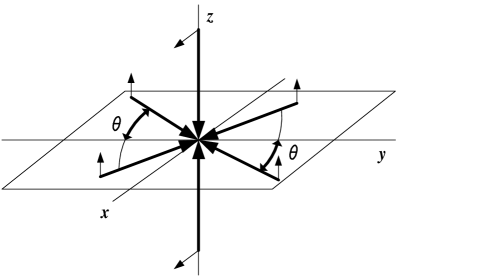
Figure 1: The lattice studied in our numerical example is formed by the interference of six laser beams. Thick arrows denote the directions of propagation of the beams, and thin arrows denote the direction of polarization. Four beams are oriented along the $x$-$y$ plane, each making an angle $\pm\theta$ with the $y$-axis and polarized along $z$. Two additional beams run parallel to $z$ and are polarized along $x$.

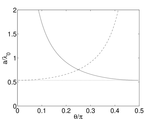
Figure 2: The lattice constants for the six-beam lattice are plotted in units of $\lambda_{0}$ as functions of $\theta$. We assume that the ratio of the resonant wavevector to that of the trapping lasers is $k_{0}/k_{L}=1.07$, consistent with the magic wavelength of ⁸⁷Sr. The solid line represents the lattice constant along $x$, the dashed line along $y$, and the constant dotted line along $z$.

As an illustration of our results, we consider ⁸⁷Sr atoms trapped in a lattice formed by six interfering beams, as shown in Fig. 1. For ⁸⁷Sr, the “magic” wavelength of the trapping lasers is roughly $\lambda_{L}=1.07\lambda_{0}$ katori02 , and one can vary the angle $\theta$ between the propagation vectors of the trapping beams. The resulting lattice is tetragonal, with lattice constants of $a_{x}=\pi/k_{L}\sin\theta$, $a_{y}=\pi/k_{L}\cos\theta$, and $a_{z}=\pi/k_{L}$ along $x$, $y$, and $z$, respectively. The lattice constants are plotted in Fig. 2. The corresponding basis of the reciprocal lattice has lengths $G_{x}=2k_{L}\sin\theta$, $G_{y}=2k_{L}\cos\theta$, and $G_{z}=2k_{L}$. We have ignored the effect of atomic back-action deutsch95 ; weidemuller98 on the trapping fields, whereby scattering of light by the atoms introduces phases that might modify the lattice constants. Such effects are expected to be stronger in red-detuned lattices, where atoms lie in the antinodes of the potential, and with increasing atomic density. Taking into account this back-action does not modify our results, except that now the lattice constants must be solved self-consistently deutsch95 ; weidemuller98 .

Using Eq. (40) we can find values of $\theta$ where constructive interference causes the shifts to be large. We focus on two specific solutions, $\theta_{0}/\pi=0.116$ and $\theta_{0}/\pi=0.180$. For our system we consider ${\langle}N{\rangle}$ atoms in a spherical distribution with uniform density $\rho({\mathbf{r}})$ for $r<r_{0}$, and zero density for $r>r_{0}$. The relationship between the density and filling fraction $P$ is given by $P=\rho({\mathbf{r}})V$, where $V$ is the volume of a unit cell. The critical value $r_{0}$ is determined by the equation

$$r_{0}=\left(\frac{3{\langle}N{\rangle}V}{4{\pi}P}\right)^{1/3}.$$ (44)

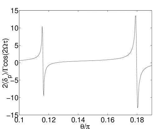
Figure 3: The calculated shifts for the six-beam lattice as a function of $\theta$. The system consists of $N=10^{6}$ atoms with a filling factor of $1$.

We first consider a perfectly filled lattice consisting of $N=10^{6}$ atoms. For simplicity we calculate the line shift to zeroth order in the interrogation time $t$. In Fig. (3), we plot the quantity $2\delta_{p}/{\Gamma}\cos(2\Omega\tau)$ as a function of $\theta$. Peaks in the shift are clearly visible at the points $\theta_{0}$ that were calculated analytically. It should be noted that the line shift can be very large in one of these “bad” configurations. Even in the limit of short interrogation times, one can see that shifts of order $\delta_{p}{\sim}10\Gamma$ are possible. This is perhaps a surprising result, and occurs because the spatial ordering of the atoms allows the interactions to behave constructively at these points. For longer interrogation times, one expects this line shift to become even larger, since the constructive interference in these configurations also leads to superradiant decay and thus a large contribution to the shift that is first order in $t$. One also sees that away from these “bad” points, the shift is strongly suppressed and even becomes zero for one particular value of $\theta$.

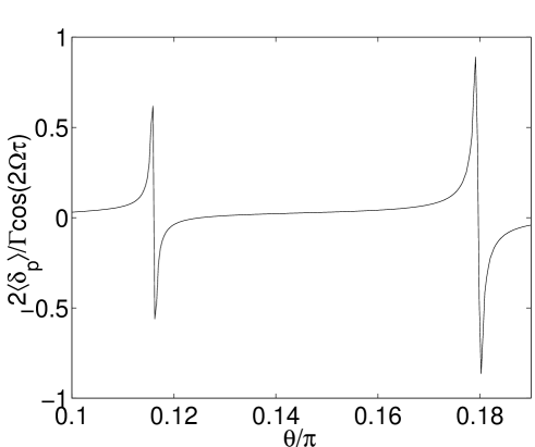
Figure 4: The calculated mean shifts for the six-beam lattice as a function of $\theta$. The system consists of ${\langle}N{\rangle}=10^{5}$ atoms with a filling factor of $0.05$.

We next consider a partially filled lattice consisting of ${\langle}N{\rangle}=10^{5}$ atoms and a filling factor of $P=0.05$. Fig. 4 gives the quantity $2{\langle}\delta_{p}{\rangle}/{\Gamma}\cos(2\Omega\tau)$ as a function of $\theta$. The mean shift ${\langle}\delta_{p}{\rangle}$ still exhibits peaks at the points $\theta_{0}$, and vanishes near $\theta/\pi=0.125$. At this “good” point, one can use Eq. (43) to estimate the variance in the expected shift. Within this diffuse approximation, we find that the variance

$$\frac{\Delta\delta_{p}}{\Gamma}{\approx}\frac{1}{2}\cos(2\Omega\tau){\times}3.1{\times}10^{-3}.$$ (45)

Experimentally, there will be additional sources of error that result from not knowing $\rho({\mathbf{r}})$ perfectly, errors in the configuration of the trapping lasers, and from the effects of atomic back-action on the lattice constants. Nonetheless, it appears that the error due to dipole-dipole interactions can be made quite small by appropriately designing the lattice.

VII Conclusion

We have derived an expression for the line shift measured in Ramsey spectroscopy due to dipole-dipole interactions. We find that the lattice geometry strongly affects the magnitude of the shift, and is peaked in lattice configurations where the interactions between atoms add constructively. Because of the spatial ordering in the lattice, the shift can be quite large in these resonant configurations. By tuning the lattice between two of these configurations, one can reduce the dipole-induced line shift to nearly zero.

While the resonant configurations might be bad for clock applications, it might be worthwhile to study these configurations further. The dipole-dipole couplings in an optical lattice offer the possibility of strong, constructive interactions that can be dynamically tuned by changing the lattice geometry. This might be useful for applications such as quantum information processing and might have interesting consequences for studying phenomena such as superradiance and for probing the superfluid-Mott insulator transition.

Appendix A Derivation of master equation

In this appendix we derive Eq. (2) starting from the full atom-field Hamiltonian. For a more detailed derivation and discussion, one can also see agarwal74 ; gross82 . The Hamiltonian for the atom-field system is

$$H=H_{0}+V,$$ (46)

where

$$H_{0} = H_{\scriptsize{\textrm{internal}}}+H_{\scriptsize{\textrm{field}}}$$ (47)

$$= \sum_{j}\left(\frac{1}{2}\hbar\omega_{0}\sigma_{j}^{z}\right)+\sum_{\mathbf{k},\hat{\epsilon}}\hbar\omega_{{\mathbf{k},\mathbf{\epsilon}}}\left(a^{\dagger}_{{\mathbf{k},\mathbf{\epsilon}}}a_{{\mathbf{k},\mathbf{\epsilon}}}+\frac{1}{2}\right)$$ (48)

and

$$V = -\sum_{j}\mathbf{d}_{j}\cdot\mathbf{E(\mathbf{r}_{j})}$$ (49)

$$= -\sum_{j}\sum_{{\mathbf{k},\mathbf{\epsilon}}}d\left(\sigma_{j}^{+}+\sigma_{j}^{-}\right)\left(\hat{\epsilon}_{\scriptsize{\textrm{atom}}}\cdot\hat{\epsilon}\right)\left(\mathcal{E}_{{\mathbf{k},\mathbf{\epsilon}}}a_{{\mathbf{k},\mathbf{\epsilon}}}e^{i\mathbf{k}\cdot\mathbf{r}_{j}}+h.c.\right).$$ (50)

$\sigma_{j}^{z}$ refers to the internal state of atom $j$, $\omega_{0}$ is the atomic transition frequency, and $\omega_{{\mathbf{k},\mathbf{\epsilon}}}$ is the frequency of the mode of the electromagnetic field with wave vector $\mathbf{k}$ and polarization $\hat{\epsilon}$. $\mathbf{r}_{j}$ is the position of atom $j$, and $\hat{\epsilon}_{\scriptsize{\textrm{atom}}}$ is the polarization direction of the dipoles.

We now consider the evolution of the atoms$+$field density matrix $\rho_{af}$ in the interaction picture. The equation of motion is given by

$$\frac{\partial\rho_{af}}{{\partial}t} = \frac{1}{i\hbar}\left[\tilde{V}(t),\rho_{af}\right],$$ (51)

$$\tilde{V}(t) = e^{iH_{0}t/\hbar}Ve^{-iH_{0}t/\hbar}.$$ (52)

We can integrate Eq. (51) once and substitute the result back into itself. We then trace out the field degrees of freedom to obtain an equation of motion for the atomic density matrix $\rho$ alone:

$$\frac{\partial\rho}{{\partial}t}=-\frac{1}{\hbar^{2}}\textrm{Tr}_{f}\int^{t}_{0}d{\tau}\left[\tilde{V}(t),\left[\tilde{V}(t-\tau),\rho_{af}(t-\tau)\right]\right].$$ (53)

To make the above equation more useful, we employ the Born-Markov approximation, replacing $\rho_{af}(t-\tau)$ with $\rho(t)\otimes\mbox{$|0\rangle$}\mbox{$\langle 0|$}$. Physically, this amounts to assuming that correlations in the field are negligible, that the field can always be approximated by a vacuum state, and that the correlation time of the atom-field system is much shorter than any atomic timescales. These assumptions safely allow us to extend the time integral to infinity, so that

$$\frac{\partial\rho}{{\partial}t}=-\frac{1}{\hbar^{2}}\textrm{Tr}_{f}\int^{\infty}_{0}d{\tau}\left[\tilde{V}(t),\left[\tilde{V}(t-\tau),\rho(t)\otimes\mbox{$|0\rangle$}\mbox{$\langle 0|$}\right]\right].$$ (54)

Writing out $\tilde{V}(t)$ and $\tilde{V}(t^{\prime})$, where $t^{\prime}=t-\tau$, give

$$\tilde{V}(t) = \sum_{a,\mathbf{k},\hat{\epsilon}}-d\mathcal{E}_{{\mathbf{k},\mathbf{\epsilon}}}\left(\hat{\epsilon}_{\scriptsize{\textrm{atom}}}\cdot\hat{\epsilon}\right)\left({\sigma_{a}^{+}}e^{i\omega_{0}t}+{\sigma_{a}^{-}}e^{-i\omega_{0}t}\right)\left(a_{{\mathbf{k},\mathbf{\epsilon}}}e^{i(\mathbf{k}{\cdot}\mathbf{r}_{a}-{\omega}_{{\mathbf{k},\mathbf{\epsilon}}}t)}+a^{\dagger}_{{\mathbf{k},\mathbf{\epsilon}}}e^{-i(\mathbf{k}{\cdot}\mathbf{r}_{a}-{\omega}_{{\mathbf{k},\mathbf{\epsilon}}}t)}\right),$$ (55)

$$\tilde{V}(t^{\prime}) = \sum_{b,\mathbf{k^{\prime}},\hat{\epsilon}^{\prime}}-d\mathcal{E}_{{\mathbf{k}^{\prime},\mathbf{\epsilon}^{\prime}}}\left(\hat{\epsilon}_{\scriptsize{\textrm{atom}}}\cdot\hat{\epsilon}^{\prime}\right)\left({\sigma_{b}^{+}}e^{i\omega_{0}t^{\prime}}+{\sigma_{b}^{-}}e^{-i\omega_{0}t^{\prime}}\right){\times}$$ (56)

$$\left(a_{{\mathbf{k}^{\prime},\mathbf{\epsilon}^{\prime}}}e^{i(\mathbf{k}^{\prime}{\cdot}\mathbf{r}_{b}-{\omega}_{{\mathbf{k}^{\prime},\mathbf{\epsilon}^{\prime}}}t^{\prime})}+a^{\dagger}_{{\mathbf{k}^{\prime},\mathbf{\epsilon}^{\prime}}}e^{-i(\mathbf{k}^{\prime}{\cdot}\mathbf{r}_{b}-{\omega}_{{\mathbf{k}^{\prime},\mathbf{\epsilon}^{\prime}}}t^{\prime})}\right).$$

When we substitute the expansions above into Eq. (54) and perform the trace, the only nonzero terms will be those associated with $a_{{\mathbf{k},\mathbf{\epsilon}}}a^{\dagger}_{{\mathbf{k}^{\prime},\mathbf{\epsilon}^{\prime}}}\mbox{$|0\rangle$}\mbox{$\langle 0|$}$, $a^{\dagger}_{{\mathbf{k},\mathbf{\epsilon}}}\mbox{$|0\rangle$}\mbox{$\langle 0|$}a_{{\mathbf{k}^{\prime},\mathbf{\epsilon}^{\prime}}}$, $a^{\dagger}_{{\mathbf{k}^{\prime},\mathbf{\epsilon}^{\prime}}}\mbox{$|0\rangle$}\mbox{$\langle 0|$}a_{{\mathbf{k},\mathbf{\epsilon}}}$, and $\mbox{$|0\rangle$}\mbox{$\langle 0|$}a_{{\mathbf{k}^{\prime},\mathbf{\epsilon}^{\prime}}}a^{\dagger}_{{\mathbf{k},\mathbf{\epsilon}}}$, where $\mathbf{k}=\mathbf{k}^{\prime}$ and $\hat{\epsilon}=\hat{\epsilon}^{\prime}$. Making these simplifications and replacing the sum on $\mathbf{k}$ by an integral gives

$$\frac{\partial\rho}{{\partial}t} = -\frac{1}{\hbar^{2}}\int^{\infty}_{0}d{\tau}\int^{\infty}_{0}\frac{1}{(2\pi)^{3}}k^{2}\,dk{\int}d\Omega\sum_{a,b,\hat{\epsilon}}d^{2}\mathcal{E}_{{\mathbf{k},\mathbf{\epsilon}}}^{2}\left(\hat{\epsilon}_{\scriptsize{\textrm{atom}}}\cdot\hat{\epsilon}\right)^{2}\left[e^{-i(\omega_{{\mathbf{k},\mathbf{\epsilon}}}-\omega_{0})\tau+i\mathbf{k}\cdot\mathbf{r}_{ab}}\sigma_{a}^{+}\sigma_{b}^{-}\rho\right.$$ (57)

$$\left.+e^{-i(\omega_{{\mathbf{k},\mathbf{\epsilon}}}+\omega_{0})\tau+i\mathbf{k}\cdot\mathbf{r}_{ab}}\sigma_{a}^{-}\sigma_{b}^{+}\rho-e^{i(\omega_{{\mathbf{k},\mathbf{\epsilon}}}+\omega_{0})\tau-i\mathbf{k}\cdot\mathbf{r}_{ab}}\sigma_{a}^{+}\rho\sigma_{b}^{-}\right.$$

$$\left.-e^{i(\omega_{{\mathbf{k},\mathbf{\epsilon}}}-\omega_{0})\tau-i\mathbf{k}\cdot\mathbf{r}_{ab}}\sigma_{b}^{-}\rho\sigma_{a}^{+}+h.c.\right].$$

The angular integral is tedious but straightforward and gives

$${\int}d\Omega\sum_{\hat{\epsilon}}e^{i\mathbf{k}\cdot\mathbf{r}_{ab}}\left(\hat{\epsilon}_{\scriptsize{\textrm{atom}}}\cdot\hat{\epsilon}\right)^{2}=4\pi\left(\sin^{2}\theta\frac{\sin{kr_{ab}}}{kr_{ab}}+\left(1-3\cos^{2}\theta\right)\left(\frac{\cos{kr_{ab}}}{(kr_{ab})^{2}}-\frac{\sin{kr_{ab}}}{(kr_{ab})^{3}}\right)\right).$$ (58)

The time integral can be evaluated using the formula

$$\int^{\infty}_{0}c\,d{\tau}e^{-ic(k{\mp}k_{0})\tau}={\pi}\delta(k_{0}{\mp}k){\pm}i\mathcal{P}\frac{1}{k_{0}{\mp}k},$$ (59)

where $\mathcal{P}$ denotes the principal value. The delta function above eventually yields the non-Hermitian component of the evolution, while the principal value yields the coherent atom-atom interactions. Performing all integrals, making the replacement $\Gamma=k_{0}^{3}d^{2}/3\pi\epsilon_{0}{\hbar}c^{3}$, and changing back to the Schrodinger picture yields Eq. (2).

Appendix B Second quantization of atoms in lattice

The results above were derived treating the atoms in the lattice in first quantization. Starting instead from second quantization, one can see that the results derived in first quantization are appropriate in the limit of tight confinement of the atoms, when the overlap between atoms at different sites can be ignored.

In second quantization, the atomic wave function $\hat{\psi}(\mathbf{r})$ can be expanded in terms of Wannier functions:

$$\hat{\psi}(\mathbf{r})=\sum_{{\nu}ni}b_{{\nu}ni}\phi_{{\nu}n}(\mathbf{r}-\mathbf{r}_{i}).$$ (60)

Here $\nu=e,g$ denotes the internal state of the atom, $n$ is the band index, and $i$ labels the lattice sites $\mathbf{r}_{i}$. To lowest order, we assume that only the harmonic oscillator ground-state wave function is relevant. The atomic Hamiltonian is then given in second quantization by

$$\hat{H}_{a}=\sum_{{\nu}ij}b_{i\nu}^{\dagger}b_{j\nu}\int{d\mathbf{r}}\phi_{\nu}(\mathbf{r}-\mathbf{r}_{i})(\frac{\hat{P}^{2}}{2M}+U(\mathbf{r})+E_{\nu})\phi_{\nu}(\mathbf{r}-\mathbf{r}_{j}).$$ (61)

In the limit of tight confinement, the overlap integrals for $i{\neq}j$ can be ignored, leading back to the atomic Hamiltonian used in first quantization.

In second quantization, the electric dipole Hamiltonian is given by

$$H_{e}=-\sum_{ij}\left(b_{ie}^{\dagger}b_{jg}\int{d\mathbf{r}}\phi_{e}(\mathbf{r}-\mathbf{r}_{i})(\mathbf{d}\cdot\mathbf{E}(\mathbf{r}))\phi_{g}(\mathbf{r}-\mathbf{r}_{j})+b_{ig}^{\dagger}b_{je}\int{d\mathbf{r}}\phi_{g}(\mathbf{r}-\mathbf{r}_{i})(\mathbf{d}\cdot\mathbf{E}(\mathbf{r}))\phi_{e}(\mathbf{r}-\mathbf{r}_{j})\right),$$ (62)

where

$$\mathbf{E}(\mathbf{r})=\sum_{{\mathbf{k},\mathbf{\epsilon}}}\mathcal{E}_{{\mathbf{k},\mathbf{\epsilon}}}a_{{\mathbf{k},\mathbf{\epsilon}}}e^{i\mathbf{k}\cdot\mathbf{r}}\hat{\epsilon}+h.c.$$ (63)

Again, in the limit of tight confinement, the overlap integrals for $i{\neq}j$ can be ignored, and furthermore the term $\mathbf{E}(\mathbf{r})$ can be replaced with $\mathbf{E}(\mathbf{r}_{i})$. In this limit this Hamiltonian is equivalent to the electric dipole Hamiltonian used in first quantization.

References

• (1) J.L. Hall, M. Zhu, and P. Buch, J. Opt. Soc. Am. B 6, 2194 (1989).
• (2) R.J. Rafac et al., Phys. Rev. Lett. 85, 2462 (2000).
• (3) H. Katori, in Proceedings of the 6th Symposium on Frequency Standards and Metrology, P. Gill, ed. (World Scientific, Singapore, 2002), pp. 323-330.
• (4) T. Mukaiyama et al., Phys. Rev. Lett. 90, 113002 (2003).
• (5) X. Xu et al., Phys. Rev. Lett. 90, 193002 (2003).
• (6) X. Xu et al., J. Opt. Soc. Am. B 20, 968 (2003).
• (7) I. Courtillot et al., physics/0303023.
• (8) T. Udem et al., Phys. Rev. Lett. 86, 4996 (2001).
• (9) G. Wilpers et al., Phys. Rev. Lett. 89, 230801 (2002).
• (10) See, for example, N. Allard and J. Kielkopf, Rev. Mod. Phys. 54, 1103 (1982).
• (11) M. Fleischhauer and S.F. Yelin, Phys. Rev. A 59, 2427 (1999).
• (12) J.D. Jackson, Classical Electrodynamics (John Wiley, New York, 1999), p. 411.
• (13) I.H. Deutsch et al., Phys. Rev. A 52, 1394 (1995).
• (14) M. Weidem$\ddot{\textrm{u}}$ller et al., Phys. Rev. A 58, 4647 (1998).
• (15) G.S. Agarwal, Springer Tracts in Modern Physics, vol. 70 (Springer, Berlin, 1974).
• (16) M. Gross and S. Haroche, Phys. Rep. 93, 301 (1982).
Refer to caption