Exact quantum jump approach to open systems in Bosonic and spin baths

Abstract

A general method is developed which enables the exact treatment of the non-Markovian quantum dynamics of open systems through a Monte Carlo simulation technique. The method is based on a stochastic formulation of the von Neumann equation of the composite system and employs a pair of product states following a Markovian random jump process. The performance of the method is illustrated by means of stochastic simulations of the dynamics of open systems interacting with a Bosonic reservoir at zero temperature and with a spin bath in the strong coupling regime.

The dynamics of open systems plays an important role in a wide variety of applications of quantum mechanics. The central goal of the physical theory TheWork is to derive tractable equations of motion for the reduced density matrix $\rho_{S}(t)$ which is defined by the trace over the environmental variables coupled to the open system. On the ground of the weak-coupling assumption the dynamics may be formulated in terms of a quantum dynamical semigroup which yields a Markovian master equation in Lindblad form ALICKI . However, strong couplings or interactions with low-temperature reservoirs give rise to large system-environment correlations which generally result in a failure of the Markov approximation: The open system dynamics develops long memory times and exhibits a pronounced non-Markovian behaviour. Important examples of non-Markovian quantum phenomena are provided by the atom laser SAVAGE , the non-perturbative decay of atoms coupled to structured reservoirs GARRAWAY , environment-induced decoherence at low temperatures, and systems interacting with a spin bath STAMP .

The non-Markovian time-development of open quantum systems represents a challenge for the analytical and the numerical treatment, since it requires to cope with a complicated integro-differential equation NZ , or with a highly non-local influence functional FEYNMAN . In the Markovian regime, Monte Carlo wave function techniques have been shown to provide efficient numerical tools SWFM . In these techniques one propagates an ensemble of stochastic state vectors $\psi(t)$ in the open system’s state space such that the reduced density matrix is recovered through the ensemble average or expectation value $\rho_{S}(t)={\mathrm{E}}(|\psi(t)\rangle\langle\psi(t)|)$. In view of the numerical efficiency of the method a generalization to the non-Markovian regime is highly desirable. One such generalization DGS is based on a complicated stochastic integro-differential equation, involving a time-integration over the past history of the system dynamics. As shown in Ref. BKP one can avoid the solution of non-local equations of motion by propagating a pair $\psi_{1}(t)$, $\psi_{2}(t)$ of stochastic state vectors and by representing the reduced system’s density matrix through the expectation value $\rho_{S}(t)={\mathrm{E}}(|\psi_{1}(t)\rangle\langle\psi_{2}(t)|)$. A similar idea has been used recently to design exact diffusion processes for systems of identical Bosons CARUSO and Fermions CHOMAZ . However, this method demands that one first derives an appropriate time-local non-Markovian master equation for the reduced system dynamics. Although this is indeed possible by use of the time-convolutionless (TCL) projection operator technique, the derivation becomes extremely complicated in the strong coupling regime which requires to take into account higher orders of the TCL expansion of the master equation. Another possibility STOCK is to exploit an explicit expression for the influence functional of the system. This method is, however, restricted to Gaussian reservoirs and linear dissipation.

In this Letter an alternative approach to the open system dynamics is developed which is based on a stochastic formulation of the von Neumann equation for the density matrix $\rho(t)$ of the total system. It is demonstrated that the motion of the state of any composite quantum system can be described through a Markovian random jump process which directly translates into a Monte Carlo simulation technique for the full non-Markovian reduced system behaviour. By contrast to previous methods which mainly deal with Bosonic reservoirs and linear dissipation, the present technique is generally applicable and does not require a specific form of the interaction between system and environment, nor any assumption on the physical properties of the environment.

In the interaction picture the Hamiltonian describing the system-environment coupling can be written as

$$H_{I}(t)=\sum_{\alpha}A_{\alpha}(t)\otimes B_{\alpha}(t),$$ (1)

where $A_{\alpha}(t)$ and $B_{\alpha}(t)$ are system and environment operators, respectively. The dynamics of the total density matrix is then governed by the von Neumann equation,

$$\frac{d}{dt}\rho(t)=-i[H_{I}(t),\rho(t)].$$ (2)

Our aim is to express $\rho(t)$ through the mean value

$$\rho(t)={\rm{E}}(|\Phi_{1}(t)\rangle\langle\Phi_{2}(t)|).$$ (3)

$|\Phi_{1}(t)\rangle$ and $|\Phi_{2}(t)\rangle$ provide a pair of state vectors of the combined system which follow an appropriate stochastic time-evolution. These state vectors are taken to be direct products of system states $\psi_{\nu}$ and environment states $\chi_{\nu}$,

$$|\Phi_{\nu}(t)\rangle=\psi_{\nu}(t)\otimes\chi_{\nu}(t),\qquad\nu=1,2.$$ (4)

Such a representation is indeed possible for any initial state $\rho(0)$ of the total system, regardless of the physical structure of open system and environment. In particular, $\rho(0)$ needs not be an uncorrelated state. Equations (3) and (4) amount to representing the density matrix of the open system through the expression

$$\rho_{S}(t)={\mathrm{tr}}_{\mathrm{B}}\rho(t)={\mathrm{E}}\left(|\psi_{1}(t)\rangle\langle\psi_{2}(t)|\langle\chi_{2}(t)|\chi_{1}(t)\rangle\right),$$ (5)

where ${\mathrm{tr}}_{\mathrm{B}}$ denotes the trace over the variables of the environment. Contrary to the standard method, expression (5) is an average over the product of $|\psi_{1}\rangle\langle\psi_{2}|$ and the overlap $\langle\chi_{2}|\chi_{1}\rangle$ of the corresponding environment states.

The task is to construct equations of motion for $\psi_{\nu}$ and $\chi_{\nu}$. We suppose that the dynamics represents a piecewise deterministic process (PDP). This is a Markovian stochastic process whose realizations consist of smooth deterministic pieces broken by instantaneous jumps occurring at random moments DAVIS . A convenient way of formulating a PDP is to write stochastic differential equations for the random variables. In our case an appropriate set of stochastic differential equations is given by

$$d\psi_{\nu} = \sum_{\alpha}\left(\frac{-i||\psi_{\nu}||}{||A_{\alpha}\psi_{\nu}||}A_{\alpha}-I\right)\psi_{\nu}dN_{\alpha\nu},$$ (6)

$$d\chi_{\nu} = \Gamma_{\nu}\chi_{\nu}dt+\sum_{\alpha}\left(\frac{||\chi_{\nu}||}{||B_{\alpha}\chi_{\nu}||}B_{\alpha}-I\right)\chi_{\nu}dN_{\alpha\nu},$$ (7)

where $I$ denotes the unit operator and

$$\Gamma_{\nu}\equiv\sum_{\alpha}\Gamma_{\alpha\nu}\equiv\sum_{\alpha}\frac{||A_{\alpha}\psi_{\nu}||\cdot||B_{\alpha}\chi_{\nu}||}{||\psi_{\nu}||\cdot||\chi_{\nu}||}.$$ (8)

Equations (6) and (7) relate the stochastic increments $d\psi_{\nu}\equiv\psi_{\nu}(t+dt)-\psi_{\nu}(t)$ and $d\chi_{\nu}\equiv\chi_{\nu}(t+dt)-\chi_{\nu}(t)$ to a set of random integers $dN_{\alpha\nu}(t)$ which are known as Poisson increments and satisfy the relations

$$dN_{\alpha\nu}(t)dN_{\beta\mu}(t) = \delta_{\alpha\beta}\delta_{\nu\mu}dN_{\alpha\nu}(t),$$ (9)

$${\mathrm{E}}(dN_{\alpha\nu}(t)) = \Gamma_{\alpha\nu}dt.$$ (10)

Equation (9) states that $dN_{\alpha\nu}(t)$ takes on the possible values $0$ or $1$, while Eq. (10) tells us that $dN_{\alpha\nu}(t)=1$ with probability $\Gamma_{\alpha\nu}dt$. Moreover, under the condition that $dN_{\alpha\nu}(t)=1$ for a particular $\alpha$ and $\nu$, all other Poisson increments vanish. According to Eqs. (6) and (7) the state vectors then perform the instantaneous jumps

$$\psi_{\nu}\rightarrow\frac{-i||\psi_{\nu}||}{||A_{\alpha}\psi_{\nu}||}A_{\alpha}\psi_{\nu},\qquad\chi_{\nu}\rightarrow\frac{||\chi_{\nu}||}{||B_{\alpha}\chi_{\nu}||}B_{\alpha}\chi_{\nu}.$$

We observe that these jumps conserve the norm of the state vectors and occur at a rate $\Gamma_{\alpha\nu}$ defined in Eq. (8). Under the condition that all Poisson increments vanish, that is $dN_{\alpha\nu}(t)=0$ for all $\alpha$, $\nu$, we have $d\psi_{\nu}=0$ and $d\chi_{\nu}=\Gamma_{\nu}\chi_{\nu}dt$. Consequently $\psi_{\nu}$ remains unchanged during $dt$, while $\chi_{\nu}$ follows a linear drift. Summarizing, $\psi_{\nu}(t)$ is a pure, norm-conserving jump process, whereas $\chi_{\nu}(t)$ is a PDP with norm-conserving jumps and a linear drift.

The stochastic differential equations (6) and (7) give rise to an equation of motion for the random matrix $R(t)=|\Phi_{1}(t)\rangle\langle\Phi_{2}(t)|$ whose expectation value is required to represent the total density matrix (see Eq. (3)). To find this equation one applies the calculus of PDPs, which is analogous to the Ito calculus of the classical theory of Brownian motion. The calculations are particularly simple in the present case since $dN_{\alpha\nu}dN_{\beta\mu}=0$ for $\nu\neq\mu$ (see Eq. (9)). This implies that the increments $|d\Phi_{1}\rangle$ and $|d\Phi_{2}\rangle$ are independent which yields $dR=|d\Phi_{1}\rangle\langle\Phi_{2}|+|\Phi_{1}\rangle\langle d\Phi_{2}|$. Substituting the expressions (4) and using the stochastic differential equations (6) and (7) as well as the relations (9) and (10) one finds

$$dR(t)=-i[H_{I}(t),R(t)]dt+dS(t),$$ (11)

where $dS=dT_{1}R+RdT_{2}^{\dagger}$ is a stochastic increment and

$$dT_{\nu}=\sum_{\alpha}\left(\Gamma_{\alpha\nu}dt-dN_{\alpha\nu}\right)\left(I+i\Gamma^{-1}_{\alpha\nu}A_{\alpha}B_{\alpha}\right).$$

Since the quantity $\Gamma_{\alpha\nu}dt-dN_{\alpha\nu}$ is zero on average by virtue of Eq. (10), we conclude that ${\mathrm{E}}(dT_{\nu})=0$ and, hence, ${\mathrm{E}}(dS)=0$. The role of the drift contributions $\Gamma_{\alpha\nu}dt$ is to compensate the mean contributions ${\mathrm{E}}(dN_{\alpha\nu})$ of the jumps towards the stochastic increment $dS$. The average over the stochastic equation (11) is therefore identical to the von Neumann equation (2). This shows that the PDP defined by Eqs. (6) and (7) indeed reproduces the exact von Neumann dynamics of the combined system through the expectation value (3).

The random process thus constructed leads to a Monte Carlo simulation technique of the open system dynamics. The numerical algorithms that can be used to generate a sample of realizations of the PDP are similar to the ones employed in the standard unraveling of quantum Markovian master equations. The decisive difference is, however, that the present method works with a pair of stochastic states and uses a representation in terms of states of the total system. Additionally, these features allow the determination of all kinds of multi-time quantum correlation functions directly from the Monte Carlo technique.

An important limitation of the Monte Carlo method is set by the size $\sigma(t)$ of the statistical fluctuations. A detailed analysis of the stochastic differential equations reveals that $\sigma(t)$ is bounded for any finite time $t$, but may eventually grow exponentially at a rate of at most $2\Gamma_{0}$, where $\Gamma_{0}$ is an upper bound for the transitions rates $\Gamma_{\nu}$. The stochastic simulation technique is thus useful for short and intermediate times, the relevant time scale being given by $1/2\Gamma_{0}$. It is impossible, in general, to use the scheme for large times, trying to beat an exponential increase of the fluctuations by enlarging the number of realizations. However, the statistical errors may be considerably reduced by employing the fact that the $|\Phi_{\nu}\rangle$ evolve independently, or by using a class of stochastic states with a more complicated structure.

To illustrate the method we first study the model of a two-state system with excited state $|e\rangle$, ground state $|g\rangle$, and transition frequency $\omega_{0}$. This system is coupled to a Bosonic reservoir consisting of a continuum of field modes $k$ with creation and annihilation operators $b^{\dagger}_{k}$, $b_{k}$, and corresponding frequency $\omega_{k}$. The interaction Hamiltonian is taken to be

$$H_{I}(t)=\sigma_{+}B(t)+\sigma_{-}B^{\dagger}(t),$$ (12)

with the system operators $\sigma_{+}=|e\rangle\langle g|$ and $\sigma_{-}=|g\rangle\langle e|$ and the reservoir operator $B(t)=\sum_{k}g_{k}b_{k}e^{i(\omega_{0}-\omega_{k})t}$. The $g_{k}$ are mode-dependent coupling constants. We investigate the dynamics evolving from the initial state $|\Phi_{\nu}(0)\rangle=\psi_{\nu}(0)\otimes\chi_{\nu}(0)=|e\rangle\otimes|0\rangle$, where $|0\rangle$ denotes the vacuum state of the reservoir. The central quantity that determines the influence of the reservoir modes on the reduced system dynamics is provided by the correlation function $\langle 0|B(t^{\prime})B^{\dagger}(t)|0\rangle$ which may be expressed in terms of the reservoir spectral density $J(\omega)$.

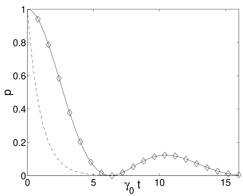
Figure 1: The excited state probability $p(t)$ of a two-state system coupled to a Bosonic reservoir: Analytical solution (continuous line) and Monte Carlo simulation of Eqs. (6), (7) (diamonds) for $\gamma_{0}/\lambda=5$ with $2\cdot 10^{7}$ realizations. The broken line shows the Born-Markov approximation.

Figure 1 shows results of a Monte Carlo simulation of the stochastic differential equations (6) and (7) for the damped Jaynes-Cummings model defined by the spectral density $J(\omega)=\frac{1}{2\pi}\gamma_{0}\lambda^{2}/[(\omega_{0}-\omega)^{2}+\lambda^{2}]$. The figure displays the population $p(t)=\langle e|\rho_{S}(t)|e\rangle$ of the excited state, estimated with the help of expression (5). For the parameter values chosen the reservoir correlation time $\lambda^{-1}$ is five times larger than the reduced system’s Markovian relaxation time $\gamma_{0}^{-1}$. This shows that the case under study belongs to the strong coupling regime and that substantial deviations from the Born-Markov dynamics occur, as is indicated in Fig. 1.

For small and intermediate couplings the reduced system dynamics is known to satisfy a non-Markovian master equation with a time-dependent generator, which can be obtained with the help of the TCL expansion in the coupling constant $\gamma_{0}/\lambda$. However, the resulting perturbation expansion of the master equation diverges in the strong coupling regime $\gamma_{0}/\lambda>0.5$ for times which are larger than the first positive zero $t_{0}$ of $p(t)$. Beyond this singularity the generator of the master equation does not exist. The TCL master equation is therefore not capable of describing the revival of the excited state population for $t>t_{0}$. By contrast, the stochastic representation developed here reproduces the exact evolution of the reduced system and, hence, correctly describes the dynamics even beyond the singularity.

The stochastic simulation method can also be applied to the dynamics of open systems interacting with a spin bath, a quantum environment whose properties differ substantially from those of a Bosonic reservoir. We examine a central spin model consisting of a spin with Pauli spin operator $\vec{\sigma}$ which is coupled to a bath of $N$ spins described by spin operators $\vec{\sigma}^{(j)}$, $j=1,2,\ldots,N$. The interaction Hamiltonian reads

$$H_{I}(t)=\sigma_{3}B_{3}+\sigma_{+}B_{-}(t)+\sigma_{-}B_{+}(t),$$ (13)

where $B_{\pm}(t)=\sum_{j}2A^{(j)}\sigma_{\pm}^{(j)}e^{\mp i\omega_{0}t}$, $B_{3}=\sum_{j}A^{(j)}\sigma_{3}^{(j)}$. This model may be used to describe the interaction of a single electron spin, confined to a quantum dot, with an external magnetic field and a bath of nuclear spins through hyperfine interactions LOSS . The transition frequency of the central spin is $\omega_{0}$ and we set $A^{(j)}=A/\sqrt{N}$, such that $A$ provides the root mean square of the couplings of the central spin to the various bath spins.

To give an example of a mixed initial state we choose $\rho(0)=|+\rangle\langle-|\otimes 2^{-N}I$, where $|\pm\rangle$ are eigenstates of the 3-component $\sigma_{3}$ of the central spin and $I$ is the unit matrix in the state space of the bath. Initially, the bath is thus in a completely unpolarized state. This state can efficiently be realized through a mixture of basis states which are simultaneous eigenstates of the square of the total spin angular momentum $\vec{J}$ of the bath and of its 3-component $J_{3}$, with an appropriate distribution of the corresponding quantum numbers $j$ and $m$. Employing an argument given in BOSE we conclude that the probability of finding the quantum numbers $(j,m)$ in the initial mixture can be written as $P(j,m)=2^{-N}\left[\binom{N}{N/2+j}-\binom{N}{N/2+j+1}\right]$. This method of generating the initial bath state bears the advantage that it enables one to employ the conservation of the 3-component $\frac{1}{2}\sigma_{3}+J_{3}$ of the total spin angular momentum and to carry out a canonical transformation which removes the term $\sigma_{3}B_{3}$ in the interaction Hamiltonian (13). This is an example of the implementation of known symmetries and conservation laws within the simulation algorithm.

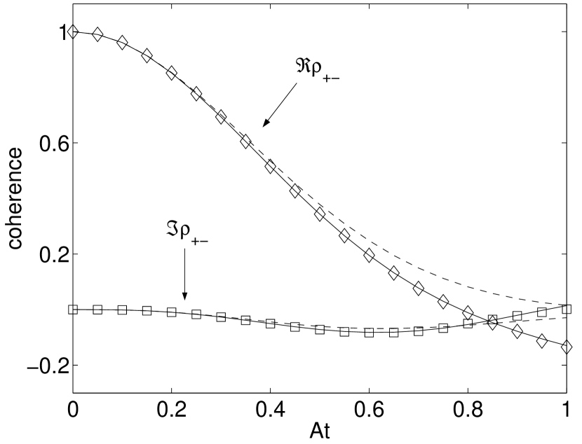
Figure 2: Real part $\Re\rho_{+-}$ and imaginary part $\Im\rho_{+-}$ of the coherence of a central spin coupled to a bath of $10^{3}$ spins through the Hamiltonian (13) with $A/\omega_{0}=0.5$. Symbols: Simulation of Eqs. (6), (7) with $2\cdot 10^{7}$ realizations. Continuous lines: Solution of the von Neumann equation (2). Broken lines: TCL master equation in second order.

Figure 2 shows the coherence $\rho_{+-}(t)=\langle+|\rho_{S}(t)|-\rangle$ of the central spin obtained from a Monte Carlo simulation employing again expression (5) for the reduced density matrix. To asses the performance of the stochastic method we compare the simulation results with the solution of the von Neumann equation for the total system. The simulation of the PDP obviously reproduces the von Neumann dynamics with high accuracy, the statistical errors of the simulation being smaller than the size of the symbols. For the parameter values chosen, the dynamics significantly deviates from the predictions of the second order TCL master equation.

The stochastic formulation naturally lends itself to several interesting generalizations. One possibility is to formulate the dynamics in imaginary time by means of the substitution $t\rightarrow-i\beta$, to examine the equilibrium properties of the system ($\beta$ denotes the inverse temperature). With slight modifications of the differential equations (6) and (7) one finds a stochastic dynamics in imaginary time which unravels the canonical density matrix of the system via the expectation value $\rho(\beta)={\mathrm{E}}(|\Phi_{1}(\beta)\rangle\langle\Phi_{2}(\beta)|)$.

It was assumed in Eq. (4) that the $|\Phi_{\nu}\rangle$ are tensor products of state vectors of system and environment. Since the interaction creates system-environment correlations it may be advantageous to employ a certain class of entangled stochastic states with the aim of a more efficient representation of $\rho(t)$ as mean value over the underlying random process. A further possibility is to use a stochastic propagation of mixed states. This is achieved, for example, by the introduction of a stochastic matrix $R(t)=|\psi_{1}(t)\rangle\langle\psi_{2}(t)|\otimes R_{\mathrm{B}}(t)$, where the $\psi_{\nu}$ are states of the open system and $R_{\mathrm{B}}$ is a random operator in the state space of the environment. It is then again possible to construct stochastic differential equations leading to the exact von Neumann dynamics with the help of the mean value $\rho(t)={\mathrm{E}}(R(t))$. A systematic exploration of these ideas could be of great relevance for the development of efficient numerical algorithm of the quantum dynamics of open systems.

References

- (1) H. P. Breuer and F. Petruccione, The Theory of Open Quantum Systems (Oxford University Press, Oxford, 2002).
- (2) R. Alicki and K. Lendi, Quantum Dynamical Semigroups and Applications, Lecture Notes in Physics 286 (Springer-Verlag, Berlin, 1987).
- (3) G. M. Moy, J. J. Hope, and C. M. Savage, Phys. Rev. A 59, 667 (1999); J. J. Hope, G. M. Moy, M. J. Collett, and C. M. Savage, Phys. Rev. A 61, 023603 (2000).
- (4) B. M. Garraway, Phys. Rev. A 55, 2290 (1997); Phys. Rev. A 55, 4636 (1997).
- (5) N. V. Prokof’ev and P. C. E. Stamp, Rep. Prog. Phys. 63, 669 (2000).
- (6) S. Nakajima, Progr. Theor. Phys. 20, 948 (1958); R. Zwanzig, J. Chem. Phys. 33, 1338 (1960).
- (7) R. P. Feynman and F. L. Vernon, Ann. Phys. (N.Y.) 24, 118 (1963); A. O. Caldeira and A. J. Leggett, Physica 121A, 587 (1983).
- (8) J. Dalibard, Y. Castin, and K. Mølmer, Phys. Rev. Lett. 68, 580 (1992); R. Dum, P. Zoller, and H. Ritsch, Phys. Rev. A 45, 4879 (1992); N. Gisin and I. C. Percival, J. Math. Phys. A: Math. Gen. 25, 5677 (1992); H. Carmichael, An Open Systems Approach to Quantum Optics, Lecture Notes in Physics m18 (Springer-Verlag, Berlin, 1993); M. B. Plenio and P. L. Knight, Rev. Mod. Phys. 70, 101 (1998); A. Imamoglu, Phys. Rev. A 50, 3650 (1994).
- (9) W. T. Strunz, L. Diòsi, and N. Gisin, Phys. Rev. Lett. 82, 1801 (1999).
- (10) H. P. Breuer, B. Kappler, and F. Petruccione, Phys. Rev. A 59, 1633 (1999).
- (11) I. Carusotto, Y. Castin, and J. Dalibard, Phys. Rev. A 63, 023606 (2001); I. Carusotto and Y. Castin, J. Phys. B: At. Mol. Opt. Phys. 34, 4589 (2001).
- (12) O. Juillet and Ph. Chomaz, Phys. Rev. Lett. 88, 142503 (2002).
- (13) J. T. Stockburger and H. Grabert, Phys. Rev. Lett. 88, 170407 (2002).
- (14) M. H. A. Davis, Markov Models and Optimization (Chapman & Hall, London, 1993).
- (15) A. V. Khaetskii, D. Loss, and L. Glazman, Phys. Rev. Lett. 88, 186802 (2002).
- (16) A. Hutton and S. Bose, quant-ph/0208114.