Quantum games of asymmetric information

Abstract

We investigate quantum games in which the information is asymmetrically distributed among the players, and find the possibility of the quantum game outperforming its classical counterpart depends strongly on not only the entanglement, but also the informational asymmetry. What is more interesting, when the information distribution is asymmetric, the contradictive impact of the quantum entanglement on the profits is observed, which is not reported in quantum games of symmetric information.

I Introduction

The field of information and computation has experienced a fundamental innovation since the last decades of the twentieth century, through the combination with the theory of quantum physics. The new-born theory of quantum information and computation opens a broad field of potential applications 1 . Its recent application into the theory of games extends the classical game theory 8 , which is in fact one of the cornerstones of modern economics, into the quantum domain. It has shown that quantum games may have great advantages over their classical counterparts 2 ; 3 ; 4 ; 6 ; g1 ; g2 ; g3 ; g4 . Many of the current works focus on games in which the players has finite number of classical strategies and/or the information is symmetrically distributed among the players. While games with continuous set of strategies and those of asymmetric information, which represent much realistic significance 5 , especially in market situations in economics, are not given much attention. However the quantization of these games deserves thorough investigations, and interesting results could be obtained.

The investigations on quantum games might provide new insights into the field of economics research, as it does in the field of computation, communication and others. There are several reasons that quantizing games that could be applied in economics may be interesting. First, market situations could be in their nature regarded as games, their quantization may be of the same interests as quantizing games 3 . Second, in any market situation, information and communication are of most importance. However, information is — as we live in a quantum world — legitimate to think of as quantum information, and communication may also need to think of as quantum communication (at least in the near future) 1 , it therefore might be interesting to investigate the quantization of market situations as games, and interesting quantum features might be explored.

In this paper we investigate the quantum form of a particular game of the market situation known as the Cournot’s Duopoly 7 of asymmetric information, based on the previously proposed physical model for continuous-variable quantum games 6 . In the quantum game of asymmetric information, the “interaction” between the quantum entanglement and the informational asymmetry creates interesting properties of the game. Due to the presence of informational asymmetry, the quantum entanglement has contradictive effects: on the one hand it promotes cooperation and potentially increases the profits, but on the other hand it potentially decreases the profits at the same time. Whether the quantum game outperforms its classical counterpart depends strongly on not only the quantum entanglement but also the informational asymmetry.

II Classical Cournot’s Duopoly of asymmetric information

We now briefly recall the classical Cournot’s Duopoly 7 of asymmetric information. In a simple scenario, firm 1 and firm 2 simultaneously choose the quantities (the strategies) $q_{1}$ and $q_{2}$, respectively, of a homogeneous product. Let $Q=q_{1}+q_{2}$ be the total quantity, and the market price be

$$P\left(Q\right)=\left\{\begin{array}[c]{ll}a-Q&\text{, for }Q\leqslant a\\ 0&\text{, for }Q>a\end{array}\right..$$ (1)

Denote the unit cost of firm 1 and 2 by $c_{1}$ and $c_{2}$ respectively, with $c_{j}<a$ ($j=1,2$). Then the profit for firm $j$ is

$$u_{j}\left(q_{1},q_{2}\right)=q_{j}\left[P\left(Q\right)-c_{j}\right],$$ (2)

with $j=1,2$. In the case of asymmetric information, firm 1 does not clearly know what $c_{2}$ (firm 2’s unit cost) is, only knows that $c_{2}=c_{H}$ with probability $\theta$ and $c_{2}=c_{L}$ with probability $1-\theta$ ($c_{H}>c_{L}$). Yet firm 2 knows with certainty the unit cost of its product ($c_{2}$) as well as that of firm 1’s ($c_{1}$). Let $q_{2H}^{\ast}$ and $q_{2L}^{\ast}$ be the quantity of firm 2 when $c_{2}=c_{H}$ and $c_{2}=c_{L}$, respectively, and $q_{1}^{\ast}$ be the quantity of firm 1. If $c_{2}=c_{H\left(L\right)}$, then firm 2 needs to set $q_{2}=q_{2H\left(L\right)}^{\ast}$ to maximize its profit

$$u_{2H\left(L\right)}\left(q_{1}^{\ast},q_{2}\right)=q_{2}[(a-q_{1}^{\ast}-q_{2})-c_{H\left(L\right)}].$$ (3)

Firm 1 needs to set $q_{1}=q_{1}^{\ast}$ to maximize its expected profit

$$u_{1}\left(q_{1},q_{2H}^{\ast},q_{2L}^{\ast}\right)=\theta u_{1}\left(q_{1},q_{2H}^{\ast}\right)+(1-\theta)u_{1}\left(q_{1},q_{2L}^{\ast}\right),$$ (4)

where

$$u_{1}(q_{1},q_{2})=q_{1}[(a-q_{1}-q_{2})-c_{1}].$$ (5)

Solving the three optimization problems yields the Bayes-Nash equilibrium 8

$$q_{1}^{\ast} =\frac{2k_{1}-k_{2}}{3},$$

$$q_{2H}^{\ast} =\frac{a+c_{1}-2c_{H}}{3}+\frac{(1-\theta)\Delta}{6},$$

$$q_{2L}^{\ast} =\frac{a+c_{1}-2c_{L}}{3}-\frac{\theta\Delta}{6},$$ (6)

where

$$k_{1} =a-c_{1},$$

$$k_{2} =a-[\theta c_{H}+(1-\theta)c_{L}],$$

$$\Delta =c_{H}-c_{L}.$$ (7)

The special instance with $k_{1}=k_{2}=k$ and $\Delta=0$ reduces to the original model of symmetric information, with the unique Nash equilibrium

$$q_{1}^{\ast}=q_{2}^{\ast}=\frac{k}{3},$$ (8)

and the payoffs being

$$u_{1}\left(q_{1}^{\ast},q_{2}^{\ast}\right)=u_{2}\left(q_{1}^{\ast},q_{2}^{\ast}\right)=\frac{k^{2}}{9}.$$ (9)

However this equilibrium fails to be the Pareto optimum 2 , which could easily be found to be

$$q_{1}^{\prime}=q_{2}^{\prime}=\frac{k}{4},$$ (10)

with

$$u_{1}(q_{1}^{\prime},q_{2}^{\prime})=u_{2}(q_{1}^{\prime},q_{2}^{\prime})=\frac{k^{2}}{8}.$$ (11)

III Quantum Cournot’s Duopoly of asymmetric information

The quantum structure is given in Fig. 1, which is the same as presented in Ref. 6 . The necessity to include continuous-variable quantum systems is that a continuous set of distinguishable states are necessary to represent all the possible outcomes of classical strategies, due to the distinguishability of classical strategies. In Fig. 1, $\left|vac\right\rangle_{1}$ and $\left|vac\right\rangle_{2}$ are two vacuum states, e.g. of two single-mode electromagnetic fields respectively belong to the two firms. $\hat{J}\left(\gamma\right)$ and $\hat{J}\left(\gamma\right)^{{\dagger}}$ are unitary operators, which are known to both firms and should be symmetric with respect to the interchange of the two firms to guarantee a fair competition. The initial state of the game is

$$\left|\psi_{i}\right\rangle=\hat{J}\left(\gamma\right)\left|vac\right\rangle_{1}\left|vac\right\rangle_{2}.$$ (12)

Strategic moves of firm $j$ is associated with unitary local operator $\hat{D}_{j}$. The final state of the game is denoted by

$$\left|\psi_{f}\right\rangle=\hat{J}\left(\gamma\right)^{\dagger}(\hat{D}_{1}\otimes\hat{D}_{2})\hat{J}\left(\gamma\right)\left|vac\right\rangle_{1}\left|vac\right\rangle_{2}.$$ (13)

Figure 1: The quantum structure of the Cournot’s Duopoly.

It is straightforward to set the final measurement be corresponding to the observables $\hat{X}_{j}=(\hat{a}_{j}^{\dagger}+\hat{a}_{j})/\sqrt{2}$ (the “position” operators) for firm $j$, where $\hat{a}_{j}^{\dagger}$ ($\hat{a}_{j}$) is the creation (annihilation) operator of firm $j$’s electromagnetic field. If the measurement result is $\tilde{x}_{j}$, then the individual quantity is determined by $q_{j}=\tilde{x}_{j}$, and hence the profit by

$$u_{j}^{Q}(\hat{D}_{1},\hat{D}_{2})=u_{j}(\tilde{x}_{1},\tilde{x}_{2}),$$ (14)

where the superscript “$Q$” denotes “quantum”. However, as will be shown in Eq. (18), in the case we considered in the present paper, the final state of the game $\left|\psi_{f}\right\rangle$ is a tensor product of two coherent states, respectively belonging to the two firms. One can not have a deterministic measurement result of $\hat{X}_{j}$, since a coherent state is not an eigenstate of $\hat{X}_{j}$. This poses a problem because the quantity $q_{j}$ is affected by uncertainty $\Delta q_{j}^{2}=\frac{1}{2}$. One possible method to reduce this uncertainty is to perform appropriate squeezing operation on the final state before the measurement according to $\hat{X}_{j}$ is carried out. The uncertainty of the measurement result of $\hat{X}_{j}$ could be reduced, at the cost of increasing the uncertainty of the measurement result of $\hat{P}_{j}$. In this paper, we assume the limit case that the state is infinitely squeezed, so that the uncertainty of the measurement result of $\hat{X}_{j}$ tends to zero. Consequently, given a coherent state $\exp(-i\tilde{x}_{j}^{\prime}\hat{P}_{j})\left|vac\right\rangle_{j}$, the final measurement could deterministically yield $q_{j}=\tilde{x}_{j}^{\prime}$ in this limit.

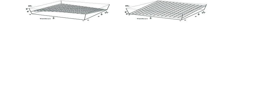
Figure 2: The profits in the iterative game with $k_{1}=k_{2}=k$, with respect to $\tanh(\gamma)$ and the amount of informational asymmetry $s$ ($\tanh(\gamma)$ monotonously maps $\gamma\in\left[0,\infty\right)$ into $\tanh(\gamma)\in\left[0,1\right)$). $\bar{u}_{1}$ is at the left and $\bar{u}_{2}$ at the right.

The classical Cournot’s Duopoly can be faithfully represented when $\hat{J}\left(\gamma\right)=\hat{J}\left(\gamma\right)^{\dagger}=I$ (the identity operator). The set

$$S_{j}=\{\hat{D}_{j}\left(x_{j}\right)=\exp(-ix_{j}\hat{P}_{j})\mid x_{j}\in\left[0,\infty\right)\}$$ (15)

is the quantum counterpart of the classical strategic space, where $\hat{P}_{j}=i(\hat{a}_{j}^{\dagger}-\hat{a}_{j})/\sqrt{2}$ (the “momentum” operators). In this paper, we restrict ourselves to the “minimal” extension, i.e. we maintain the strategic space unexpanded ($S_{j}$ for firm $j$) while only extend the initial state $\left|\psi_{i}\right\rangle$ to be entangled. This minimal extension guarantees that any features of the game not seen in the classical form could be completely due to the quantum entanglement. However it is also possible to find a quantum version that includes both the entangled state and the expanded strategic spaces.

The choice of the entangling operator is not unique. Even though the requirement that for vanishing entanglement the classical game should be reproduced can not uniquely specify this operator in the case presented in this paper. However a possible and legitimate one is

$$\hat{J}\left(\gamma\right)=e^{-\gamma(\hat{a}_{1}^{\dagger}\hat{a}_{2}^{\dagger}-\hat{a}_{1}\hat{a}_{2})}=e^{i\gamma(\hat{X}_{1}\hat{P}_{2}+\hat{X}_{2}\hat{P}_{1})}.$$ (16)

The initial state is exactly the two-mode squeezed vacuum state

$$\left|\psi_{i}\right\rangle=\exp\{-\gamma(\hat{a}_{1}^{\dagger}\hat{a}_{2}^{\dagger}-\hat{a}_{1}\hat{a}_{2})\}\left|vac\right\rangle_{1}\left|vac\right\rangle_{2},$$ (17)

where $\gamma\geqslant 0$ is known as the squeezing parameter and can be reasonably regarded as a measure of entanglement. Detailed calculation reveals that if firm $j$’s strategy is $\hat{D}_{j}\left(x_{j}\right)=\exp(-ix_{j}\hat{P}_{j})$, then the final state is

$$\left|\psi_{f}\right\rangle= \exp\{-i(x_{1}\cosh\gamma+x_{2}\sinh\gamma)\hat{P}_{1}\}\left|vac\right\rangle_{1}$$

$$\otimes\exp\{-i(x_{2}\cosh\gamma+x_{1}\sinh\gamma)\hat{P}_{2}\}\left|vac\right\rangle_{2}.$$ (18)

Hence the quantities read out from the final measurement are

$$q_{1} =x_{1}\cosh\gamma+x_{2}\sinh\gamma,$$

$$q_{2} =x_{2}\cosh\gamma+x_{1}\sinh\gamma.$$ (19)

The total quantity is $Q=q_{1}+q_{2}=e^{\gamma}\left(x_{1}+x_{2}\right)$, and the market price is $P=a-e^{\gamma}\left(x_{1}+x_{2}\right)$. Therefore profits are

$$u_{1}^{Q}\left(x_{1},x_{2}\right) =\left(x_{1}\cosh\gamma+x_{2}\sinh\gamma\right)\left[P-c_{1}\right],$$

$$u_{2H\left(L\right)}^{Q}\left(x_{1},x_{2}\right) =\left(x_{2}\cosh\gamma+x_{1}\sinh\gamma\right)\left[P-c_{H\left(L\right)}\right],$$ (20)

here for convenience we directly denote the strategy by $x_{j}$ when it is $\hat{D}_{j}\left(x_{j}\right)$.

Let $\{x_{1}^{\ast},x_{2H}^{\ast},x_{2L}^{\ast}\}$ be the Bayes-Nash equilibrium. Then $x_{2}=x_{2H\left(L\right)}^{\ast}$ is chosen to maximize $u_{2H\left(L\right)}^{Q}(x_{1}^{\ast},x_{2})$, and $x_{1}=x_{1}^{\ast}$ is chosen to maximize $\theta u_{1}^{Q}\left(x_{1},x_{2H}^{\ast}\right)+(1-\theta)$ $u_{1}^{Q}\left(x_{1},x_{2L}^{\ast}\right)$. Solving the three optimization problem yields the Bayes-Nash equilibrium 8 and the profits could also be obtained. For convenience and simplicity, we further set $k_{1}=k_{2}=k$. Detailed calculation gives the unique Bayes-Nash equilibrium as

$$x_{1}^{\ast} =\frac{k\cosh\gamma}{1+2e^{2\gamma}},$$

$$x_{2H}^{\ast} =\frac{k-\left(1-\theta\right)\Delta+e^{2\gamma}\left[k-2\left(1-\theta\right)\Delta\right]}{2e^{\gamma}\left(1+2e^{2\gamma}\right)},$$

$$x_{2L}^{\ast} =\frac{k+\theta\Delta+e^{2\gamma}\left[k+2\theta\Delta\right]}{2e^{\gamma}\left(1+2e^{2\gamma}\right)}.$$ (21)

In the remaining part of this paper, we would like to consider an iterative game in which the unit cost of firm 2’s product is determined by the probability known by firm 1, i.e. $c_{H}$ with probability $\theta$ and $c_{L}$ with probability $1-\theta$, to avoid the ambiguity and complexity caused by the specific choice of firm 2’s unit cost in a single game. The average profits in the iterative game are

$$\bar{u}_{1}\left(\gamma,s\right) =\theta u_{1}^{Q}\left(x_{1}^{\ast},x_{2H}^{\ast}\right)+\left(1-\theta\right)u_{1}^{Q}\left(x_{1}^{\ast},x_{2L}^{\ast}\right)$$

$$=\frac{k^{2}}{8}\left[\frac{8e^{\gamma}\cosh\gamma}{(3\cosh\gamma+\sinh\gamma)^{2}}+\left(e^{-2\gamma}-1\right)s\right],$$

$$\bar{u}_{2}\left(\gamma,s\right) =\theta u_{2H}^{Q}\left(x_{1}^{\ast},x_{2H}^{\ast}\right)+\left(1-\theta\right)u_{2L}^{Q}\left(x_{1}^{\ast},x_{2L}^{\ast}\right)$$

$$=\bar{u}_{1}\left(\gamma,s\right)+\frac{k^{2}}{4}s,$$ (22)

where

$$s=\theta\left(1-\theta\right)\frac{\Delta^{2}}{k^{2}}\geqslant 0.$$ (23)

The profits are already expressed as functions of $\gamma$ and $s$, and are plotted in Fig. 2.

The notation $s$ defined in Eq. (23) can reasonably be regarded as the amount of informational asymmetry. Indeed, $s=0$ is attained only when $\theta=0$, $\theta=1$, or $\Delta=0$, each corresponding to the case where firm 1 has the perfect information about firm 2’s unit cost, i.e. there is no asymmetry in the information distribution. However for fixed $\theta$, $s$ increases as $\Delta$ increases, and for fixed $\Delta$, $s$ increases as $\theta$ approaches $1/2$. This means that the more asymmetrical the information distribution is, the larger is $s$. It is in this sense that we regard $s$ as a measure of the informational asymmetry of the game.

We now investigate how the profits depend on the entanglement and the amount of informational asymmetry. The derivative of $\bar{u}_{1}$ and $\bar{u}_{2}$ with respect to $\gamma$ is

$$\frac{\partial\bar{u}_{1}}{\partial\gamma}=\frac{\partial\bar{u}_{2}}{\partial\gamma}=\frac{e^{-2\gamma}k^{2}}{4}\left[\frac{4e^{\gamma}}{(3\cosh\gamma+\sinh\gamma)^{3}}-s\right].$$ (24)

Eq. (24) shows that there is a threshold for the amount of informational asymmetry, $s_{m}=4/27$. If $s>s_{m}$,

$$\frac{\partial\bar{u}_{1}}{\partial\gamma}=\frac{\partial\bar{u}_{2}}{\partial\gamma}<0,$$ (25)

which means the profits monotonously decrease as $\gamma$ increases. In this case, the quantum game is definitely inferior to the classical game. It is also interesting to see that if $s>1$ we can always find that for some value of $\gamma$, $\bar{u}_{1}$ will be less than zero while $\bar{u}_{2}$ remains positive. In this case, lacking information makes firm 1 lose money in business on average, yet it is beyond firm 1’s means to get out of it.

In the case that $s<s_{m}$,

$$\left.\frac{\partial\bar{u}_{1}}{\partial\gamma}\right|_{\gamma=0}=\left.\frac{\partial\bar{u}_{2}}{\partial\gamma}\right|_{\gamma=0}>0,$$ (26)

the profits increase as $\gamma$ increases when $\gamma$ is small. However we can find $\gamma_{m}$ satisfying

$$\left.\frac{\partial\bar{u}_{1}}{\partial\gamma}\right|_{\gamma=\gamma_{m}}=\left.\frac{\partial\bar{u}_{2}}{\partial\gamma}\right|_{\gamma=\gamma_{m}}=0,$$ (27)

hence $\bar{u}_{1}$ and $\bar{u}_{2}$ simultaneously reach the maximum at $\gamma=\gamma_{m}$. But when $\gamma>\gamma_{m}$ the profits decrease.

In the limit that $\gamma\rightarrow+\infty$, we have

$$\left.\bar{u}_{1}(\gamma,s)\right|_{\gamma\rightarrow+\infty} =\frac{k^{2}(1-s)}{8},$$

$$\left.\bar{u}_{2}(\gamma,s)\right|_{\gamma\rightarrow+\infty} =\frac{k^{2}(1+s)}{8}.$$ (28)

While in the classical game $\gamma=0$,

$$\bar{u}_{1}(0,s) =\frac{k^{2}}{9},$$

$$\bar{u}_{1}(0,s) =k^{2}(\frac{1}{9}+\frac{s}{4}),$$ (29)

therefore if $1/9<s<s_{m}$, we can find $\gamma_{c}>0$ satisfying

$$\bar{u}_{1}(\gamma_{c},s) =\bar{u}_{1}(0,s),$$

$$\bar{u}_{2}(\gamma_{c},s) =\bar{u}_{2}(0,s).$$ (30)

Thus we find another threshold for the amount of informational asymmetry, $s_{c}=1/9<s_{m}$.

For $s<s_{c}$, $\left.\bar{u}_{1}(\gamma,s)\right|_{\gamma\rightarrow+\infty}>\bar{u}_{1}(0,s)$ and $\left.\bar{u}_{2}(\gamma,s)\right|_{\gamma\rightarrow+\infty}>\bar{u}_{2}(0,s)$, the quantum game is always superior to the classical game for any $\gamma>0$. For $s_{c}<s<s_{m}$, the quantum game is superior to the classical game for $0<\gamma<\gamma_{c}$ but inferior for $\gamma>\gamma_{c}$, and the profits reach the maximum at $\gamma=\gamma_{m}<\gamma_{c}$. While for $s>s_{m}$, the quantum game is definitely inferior to the classical game, and the profits will get worse when the entanglement increases. To be illustrative, we plot firm 1’s profit (divided by $k^{2}$) with different settings of $s$ in Fig. 3, in which all the above intriguing features could be seen.

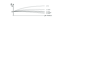
Figure 3: The $\bar{u}_{1}/k^{2}$ versus $\tanh(\gamma)$ plot with $k_{1}=k_{2}=k$. The solid lines are associated with the values of $s$. The horizontal dashed line at $\bar{u}_{1}/k^{2}=1/9$ represents the classical profit.

In fact the profits in Eq. (22) consist of two parts: one is independent of $s$, the other is linear with $s$. The first part is an increasing function of $\gamma$ while the second is a decreasing one. The combination of these two parts creates the intriguing features as mentioned above. However it also implies that the quantum entanglement has contradictive effects on the game with asymmetric information: on the one hand it potentially increases the profits but on the other hand it potentially decreases it. The part independent of $s$ in Eq. (22) can be regarded as the representation of cooperation. As the entanglement increases, the cooperation increases and the profits potentially increases. While the part dependent of $s$ in Eq. (22) represents the impact of the informational asymmetry. This impact will decrease the payoff with the presence of entanglement, not only for the player who lacks information but also for the one who possesses more information.

A special instance is the case with $s=0$ (see in Ref. 6 ), in which the classical game turns back to the original one of symmetric information proposed by Cournot 7 . While in the maximally entangled limit with $\gamma\rightarrow+\infty$, we have $\left.\bar{u}_{1}(\gamma,0)\right|_{\gamma\rightarrow+\infty}=\left.\bar{u}_{2}(\gamma,0)\right|_{\gamma\rightarrow+\infty}\rightarrow k^{2}/8$, which is exactly the Pareto optimum. In this case the initial state tends towards the singular limit ${\textstyle\int}\left|x,-x\right\rangle$d$x$. It is this limiting state, first considered by Einstein, Podolsky and Rosen, which enables the two firms to best cooperate, and therefore to be best rewarded. The dilemma-like situation is thus completely removed in this limit.

IV Conclusion

We investigated the quantization of a game of a market situation known as the Cournot’s Duopoly of asymmetric information, based on the continuous-variable model for quantum games given in Ref. 6 . We found that, with the presence of informational asymmetry, the quantum entanglement has contradictive effects. On the one hand the quantum entanglement promotes cooperation and potentially increases the profits. While on the other hand, due to the asymmetric distribution of information, the quantum entanglement induces a decreasing effect not only to the player who lacks information but also to the one who possesses more information. The combination of these two effects results in an intriguing variation of the game with respect to the measure of entanglement and the amount of informational asymmetry.

- (1) The Physics of Quantum Information, edited by D. Bouwmeester, A. Ekert, and A. Zeilinger (Springer, New York, 2000).
- (2) P. D. Straffin, Game Theory and Strategy (The Mathematical Association of America, 1993).
- (3) D. A. Meyer, Phys. Rev. Lett. 82, 1052 (1999).
- (4) J. Eisert et al., Phys. Rev. Lett. 83, 3077 (1999).
- (5) J. Du et al., Phys. Rev. Lett. 88, 137902 (2002); Phys. Lett. A 289, 9 (2001); Phys. Lett. A 302, 229 (2002).
- (6) H. Li, J. Du and S. Massar, Phys. Lett. A 306, 73 (2002).
- (7) S. C. Benjamin and P. M. Hayden, Phys. Rev. A 64, 030301 (2001); N. F. Johnson, Phys. Rev. A 63, 020302 (2001).
- (8) L. Marinatto and T. Weber, Phys. Lett. A 272, 291 (2000); J. L. Chen et al., Phys. Rev. A 65, 052320 (2002).
- (9) A. Iqbal and A. H. Toor, Phys. Rev. A 65, 022306 (2002); Phys. Rev. A 65, 052328 (2002).
- (10) A. P. Flitney and D. Abbott, Phys. Rev. A 65, 062318 (2002); W. Y. Hwang, D. Ahn, and S. W. Hwang, Phys. Rev. A 64, 064302 (2001).
- (11) P. Ball, Economics Nobel 2001, Science Update, 16 Oct. 2001.
- (12) A. Cournot, in Researches Into the Mathematical Principles of the Theory of Wealth (Macmillan, New York, 1897).