Tomography of entangled massive particles

Abstract

We report on tomographic means to study the stability of a qubit register based on a string of trapped ions. In our experiment, two ions are held in a linear Paul trap and are entangled deterministically by laser pulses that couple their electronic and motional states. We reconstruct the density matrix using single qubit rotations and subsequent measurements with near-unity detection efficiency. This way, we characterize the created Bell states, the states into which they subsequently decay, and we derive their entanglement, applying different entanglement measures.

Quantum state tomographyvogel allows the estimation of an unknown quantum state that is available in many identical copies. It has been experimentally demonstrated for a variety of physical systems, among them the quantum state of a light modeSmithey , the vibrational state of a moleculeDunn and a single ionLeibfried , and the wave packets of atoms of an atomic beamKurtsiefer . Multi-particle states have been investigated in nuclear magnetic resonance experimentsChuang as well as in experiments involving entangled photon pairsWhite1 ; White2 . However, no experiment to date has completely reconstructed the quantum state of entangled massive particles Hagley ; Turchette ; Kielpinski ; FSK . In the context of quantum information theoryNielsen , multi-particle entangled states are considered to be an essential resource for processing information encoded in quantum states (qubits). Many protocols require the deterministic creation of entangled states and the preservation of these states over times much longer than their production time. For experiments aiming at entangling qubits, the coupling of the qubits to the environment needs to be well understood so that its effect can be minimized.

In this article, we describe the deterministic creation of all four two-ion Bell states, i.e. $\Psi_{\pm}=(|10\rangle\pm|01\rangle)\sqrt{2}$ and $\Phi_{\pm}=(|11\rangle\pm|00\rangle)\sqrt{2}$, where $|x_{1}x_{2}\rangle,\;x_{i}\in\{0,1\}$ represents the combined state of the two qubits. By tomographically reconstructing the two-ion density matrix, we fully characterize these states and determine their entanglement by different means. We also measure the time evolution of these states and determine the decay of their entanglement.

In our experiments, a qubit is encoded in a superposition of internal states of a calcium ion. We use the $|S_{1/2},m=-1/2\rangle$ ground state and the metastable $|D_{5/2},m=-1/2\rangle$ state (lifetime $\tau\sim 1$ s) to represent the qubit states $|1\rangle$ and $|0\rangle$, respectively. Two ${}^{40}{\rm Ca}^{+}$ ions are loaded into a linear Paul trap having vibrational frequencies of $(2\pi)1.2$ MHz in the axial and $(2\pi)5$ MHz in the transverse directions. After 10 ms of Doppler and sideband cooling Roos , the ions’ breathing mode of axial vibration at $\omega_{\rm b}=(2\pi)\sqrt{3}\times 1.2$ MHz is cooled to the ground state $|0_{\rm b}\rangle$ ( 99% occupation). Thereafter, the qubits are initialized in the $|11\rangle$ state. For quantum state engineering, we employ a narrowband Ti:Sapphire laser which is tightly focussed onto either one of the two ions. By exciting the $S_{1/2}$ to $D_{5/2}$ quadrupole transition near 729 nm ($\gamma=0.16$ Hz), we prepare a single ion in a superposition of the $|0\rangle$ and $|1\rangle$ states. If the laser excites the transition on resonance (”carrier transition“), the ion’s vibrational state is not affected whereas if the laser frequency is set to the transition’s upper motional sideband (”blue sideband“), the electronic states become entangled with the motional states $|0_{\rm b}\rangle$ and $|1_{\rm b}\rangle$ of the breathing mode. We use an acousto-optical modulator to switch between carrier and sideband transition frequency and to control the phase of the light field FSK ; Roos ; FSK2 ; Haeffner . An electro-optical beam deflector switches the laser beam from one ion, over a distance of 5.3 $\mu$m, to the other ion within 15 $\mu$s. Directing the beam which has a width of 2.5 $\mu$m (FWHM at the focus) onto one ion, the intensity on the neighboring ion is suppressed by a factor of $2.5\cdot 10^{-3}$. By a sequence of laser pulses of appropriate length, frequency, and phase, the two ions are prepared in a Bell state as described below. For detection of the internal quantum states, we excite the $S_{1/2}$ to $P_{1/2}$ dipole transition near 397 nm and monitor the fluorescence for 15 ms with an intensified CCD camera separately for each ion. Fluorescence indicates that the ion was in the $S_{1/2}$ state, no fluorescence reveals that it was in the $D_{5/2}$ state. By repeating the experimental cycle 200 times we find the average populations of all product basis states $|00\rangle$, $|01\rangle$, $|10\rangle$ and $|11\rangle$.

We create a Bell state by applying laser pulses to ion 1 and 2 on the blue sideband and the carrier. Using the Pauli spin matrices $\sigma_{x}$,$\sigma_{y}$,$\sigma_{z}$eigenvectornote and the operators $b$ and $b^{\dagger}$ that annihilate and create a phonon in the breathing mode, we denote single qubit carrier rotations of qubit $\alpha$ by

$$R_{\alpha}(\theta,\phi)=\exp\left[i\frac{\theta}{2}\left(\sigma_{x}^{(\alpha)}\cos\phi-\sigma_{y}^{(\alpha)}\sin\phi\right)\right]$$ (1)

and rotations on the blue sideband of the vibrational breathing mode by

$$R_{\alpha}^{+}(\theta,\phi)=\exp\left[i\frac{\theta}{2}\left(\sigma_{x}^{(\alpha)}b^{\dagger}\cos\phi-\sigma_{y}^{(\alpha)}b\sin\phi\right)\right].$$ (2)

Now, we produce the Bell state $\Psi_{\pm}=(|10\rangle\pm|01\rangle)/\sqrt{2}$ by the pulse sequence $U_{\Psi_{\pm}}=R_{2}^{+}(\pi,\pm\pi/2)R_{2}(\pi,\pi/2)R_{1}^{+}(\pi/2,-\pi/2)$ applied to the $|11\rangle$ state. The pulse $R_{1}^{+}(\pi/2,-\pi/2)$ entangles the motional and the internal degrees of freedom, the next two pulses $R_{2}^{+}(\pi,\pm\pi/2)R_{2}(\pi,\pi/2)$ map the motional degree of freedom onto the internal state of ion 2. Appending another $\pi$-pulse, $U_{\Phi_{\pm}}=R_{2}(\pi,0)U_{\Psi\pm}$, produces the state $\Phi_{\pm}$ up to a global phase. The pulse sequence takes less than 200 $\mu$s.

To account for experimental imperfections, we describe the quantum state by a density matrix $\rho$. For its experimental determination we expand $\rho$ into a superposition $\rho=\sum\nolimits_{i}\lambda_{i}O_{i}$ of mutually orthogonal Hermitian operators $O_{i}$, which form a basis and obey the equation ${\rm tr}(O_{i}O_{j})=4\delta_{ij}$Fano . Then, the coefficients $\lambda_{i}$ are related to the expectation values of $O_{i}$ by $\lambda_{i}={\rm tr}(\rho O_{i})/4$. For a two-qubit system, a convenient set of operators is given by the 16 operators $\sigma_{i}^{(1)}\otimes\sigma_{j}^{(2)}$, $(i,j=0,1,2,3)$, where $\sigma_{i}^{(\alpha)}$ runs through the set of Pauli matrices ${1,\sigma_{x},\sigma_{y},\sigma_{z},}$ of qubit $\alpha$.

The reconstruction of the density matrix $\rho$ is now accomplished by measuring the expectation values $\langle\sigma_{i}^{(1)}\otimes\sigma_{j}^{(2)}\rangle_{\rho}$. A fluorescence measurement projects the quantum state into one of the states $|x_{1}x_{2}\rangle$, $x_{i}\in\{0,1\}$. By repeatedly preparing and measuring the quantum state, we obtain the average population in states $|x_{1}x_{2}\rangle$ from which we calculate the expectation values of $\sigma_{z}^{(1)}$, $\sigma_{z}^{(2)}$ and $\sigma_{z}^{(1)}\otimes\sigma_{z}^{(2)}$. To measure operators involving $\sigma_{y}$, we apply a transformation U that maps the eigenvectors of $\sigma_{y}$ onto the eigenvectors of $\sigma_{z}$, i.e. $U\sigma_{y}U^{-1}=\sigma_{z}$, where $U=R(\pi/2,\pi)$. Similarly, the operator $\sigma_{x}$ is transformed into $\sigma_{z}$ by choosing $U=R(\pi/2,3\pi/2)$. Therefore, all expectation values can be determined by measuring $\sigma_{z}^{(1)}$, $\sigma_{z}^{(2)}$ or $\sigma_{z}^{(1)}\otimes\sigma_{z}^{(2)}$. To obtain all 16 expectation values, nine different settings have to be used (see table 1).

Table 1: Additional pulses used for reconstructing a two-qubit quantum state. All expectation values needed for quantum state reconstruction can be determined by applying either one of the nine different transformations given in the table below and subsequently measuring the qubit state. Only the expectation values of the operators displayed in bold face are used to reconstruct the quantum state.

	Transformation applied to		Measured
	ion 1	ion 2	expectation values
1	-	-	$\bm{\sigma_{z}^{(1)}}$	$\bm{\sigma_{z}^{(2)}}$	$\bm{\sigma_{z}^{(1)}\otimes\sigma_{z}^{(2)}}$
2	$R(\pi/2,3\pi/2)$	-	$\bm{\sigma_{x}^{(1)}}$	$\sigma_{z}^{(2)}$	$\bm{\sigma_{x}^{(1)}\otimes\sigma_{z}^{(2)}}$
3	$R(\pi/2,\pi)$	-	$\bm{\sigma_{y}^{(1)}}$	$\sigma_{z}^{(2)}$	$\bm{\sigma_{y}^{(1)}\otimes\sigma_{z}^{(2)}}$
4	-	$R(\pi/2,3\pi/2)$	$\sigma_{z}^{(1)}$	$\bm{\sigma_{x}^{(2)}}$	$\bm{\sigma_{z}^{(1)}\otimes\sigma_{x}^{(2)}}$
5	-	$R(\pi/2,\pi)$	$\sigma_{z}^{(1)}$	$\bm{\sigma_{y}^{(2)}}$	$\bm{\sigma_{z}^{(1)}\otimes\sigma_{y}^{(2)}}$
6	$R(\pi/2,3\pi/2)$	$R(\pi/2,3\pi/2)$	$\sigma_{x}^{(1)}$	$\sigma_{x}^{(2)}$	$\bm{\sigma_{x}^{(1)}\otimes\sigma_{x}^{(2)}}$
7	$R(\pi/2,3\pi/2)$	$R(\pi/2,\pi)$	$\sigma_{x}^{(1)}$	$\sigma_{y}^{(2)}$	$\bm{\sigma_{x}^{(1)}\otimes\sigma_{y}^{(2)}}$
8	$R(\pi/2,\pi)$	$R(\pi/2,3\pi/2)$	$\sigma_{y}^{(1)}$	$\sigma_{x}^{(2)}$	$\bm{\sigma_{y}^{(1)}\otimes\sigma_{x}^{(2)}}$
9	$R(\pi/2,\pi)$	$R(\pi/2,\pi)$	$\sigma_{y}^{(1)}$	$\sigma_{y}^{(2)}$	$\bm{\sigma_{y}^{(1)}\otimes\sigma_{y}^{(2)}}$

Since a finite number of experiments allow only for an estimation of the expectation values $\langle\sigma_{i}^{(1)}\otimes\sigma_{j}^{(2)}\rangle_{\rho}$, the reconstructed matrix $\rho_{\rm R}$ is not guaranteed to be positive semi-definiteHradil . Therefore, we employ a maximum likelihood estimation of the density matrixHradil ; Banaszek , following the procedure as suggested and implemented in refs. Banaszek ; James . We parametrize the density matrix by the elements of the Cholesky matrix T related to $\rho$ by $\rho=T^{\dagger}T$. Since the reconstructed density matrix $\rho_{R}$ can have negative eigenvalues, we cannot use $\rho_{R}$ as a starting point for the optimization routine. Instead, we use $\rho_{P}=P\rho_{R}P/tr(P\rho_{R}P)$ where P projects onto the subspace spanned by the eigenvectors of $\rho_{R}$ having non-negative eigenvalues.

For the pulse sequence that is designed to produce the state $\Psi_{+}=(|10\rangle+|01\rangle)/\sqrt{2}$, we obtain the density matrix $\rho_{\Psi_{+}}$ shown in Fig. 1a. The fidelity $F$ of the reconstructed state is $F=\langle\Psi_{+}|\rho_{\Psi_{+}}|\Psi_{+}\rangle=0.91$. To produce the state $\rho_{\Psi_{-}}=(|10\rangle-|01\rangle)/\sqrt{2}$, we change the phase of the sideband $\pi$-pulse by $\pi$ and experimentally obtain the density matrix $\rho_{\Psi_{-}}$ shown in Fig. 1b. For $\Phi_{\pm}=(|11\rangle\pm|00\rangle)/\sqrt{2}$, we find the density matrices depicted in Fig. 1c and d.

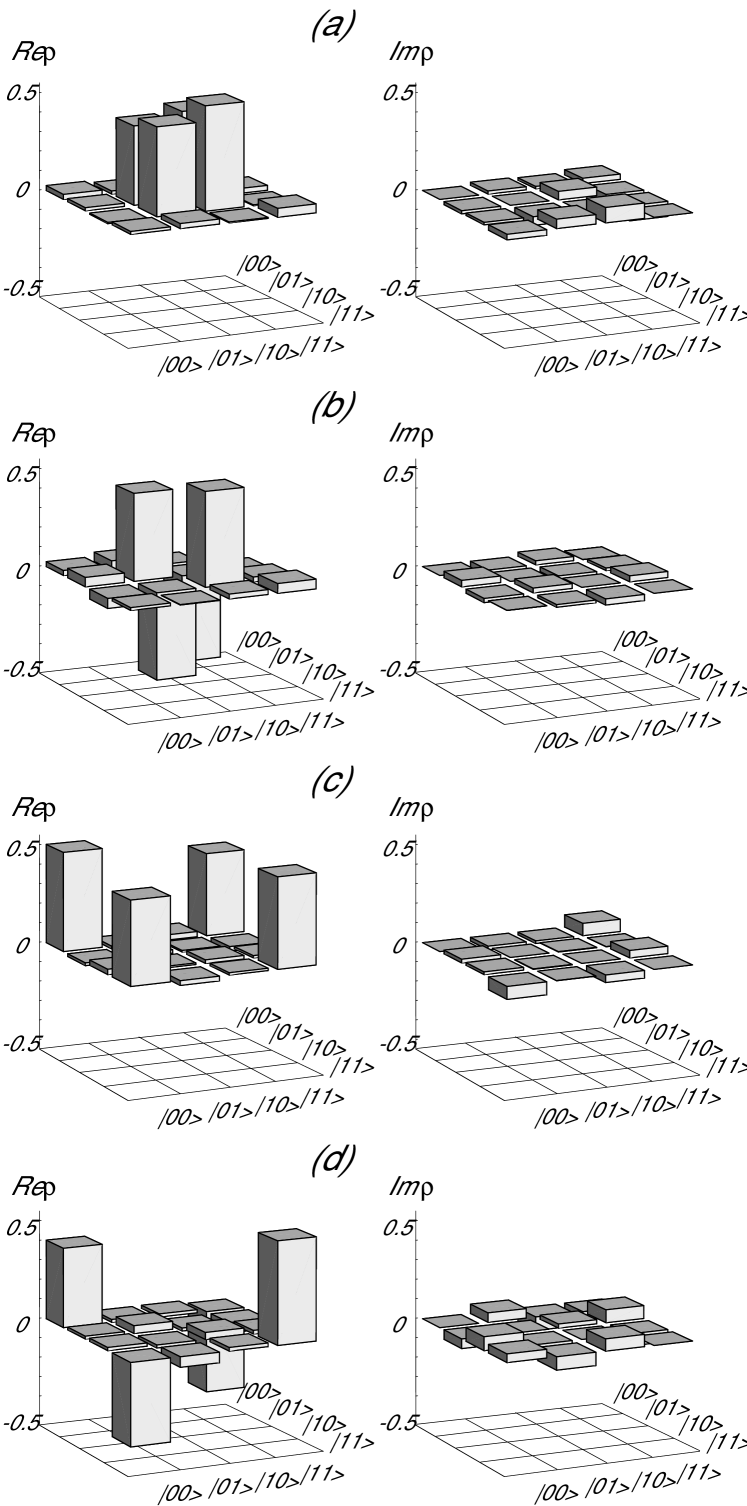
Figure 1: (a): Real and imaginary part of the density matrix $\rho_{\Psi_{+}}$ that approximates $\Psi_{+}=(|10\rangle+|01\rangle)/\sqrt{2}$. The measured fidelity is $F_{\Psi_{+}}=\langle\Psi_{+}|\rho_{\Psi_{+}}|\Psi_{+}\rangle=0.91$. (b): Real and imaginary part of the density matrix $\rho_{\Psi_{-}}$ that approximates $\Psi_{-}=(|10\rangle-|01\rangle)/\sqrt{2}$. The measured fidelity is $F_{\Psi_{-}}=0.90$. (c),(d): Density matrix elements of $\rho_{\Phi_{+}}$ (c) and $\rho_{\Phi_{-}}$ (d). Here, $F_{\Phi_{+}}=0.91$ and $F_{\Phi_{-}}=0.88$.

Having reconstructed a Bell state’s density matrix, we can now check that the two qubits are indeed entangled. It has been shown that a mixed state $\rho$ of two qubits is entangled if and only if its partial transpose $\rho^{PT}$ has a negative eigenvaluePeres ; Horodecki . Not surprisingly, the partial transpose of the density matrix $\rho_{\Psi_{+}}$ (Fig. 1a) has eigenvalues $\{-0.42(2),0.40(2),0.49(2),0.53(3)\}$ close to the values of a maximally entangled state $\{-0.5,0.5,0.5,0.5\}$. Errors in the determination of the density matrix elements and of quantities derived from them occur mainly as a consequence of quantum projection noise. Systematic effects like pulse length errors or addressing errors (coherent excitation of an ion by stray light) play a minor role. We estimate the magnitude of quantum projection noise by a bootstrapping technique Efron where the reconstructed density matrix serves for calculating probability distributions used in a Monte-Carlo simulation of our experiment.

Among the different measures put forward to quantify the entanglement of mixed bipartite states, the entanglement of formation, $E$, has the virtue of being analytically calculable from the density matrix of a two-qubit system. For a separable state, $E=0$, whereas $E=1$ for a maximally entangled state. Using the formula given by WoottersWotters , we find $E(\rho_{\Psi_{+}})=0.79(4)$. For the density matrices that nominally correspond to the Bell states $\Psi_{-}$ and $\Phi_{\pm}$, we measure $E(\rho_{\Psi_{-}})=0.75(5)$, $E(\rho_{\Phi_{+}})=0.76(4)$ and $E(\rho_{\Phi_{-}})=0.72(5)$.

All of these Bell states violate a Clauser-Horne-Shimony-Holt inequality. For the state $\rho_{\Psi_{+}}$, for example, we obtain $|\langle A\rangle|=2.52(6)>2$, where we have introduced the operator $A=\sigma_{x}^{(1)}\otimes\sigma_{x-z}^{(2)}+\sigma_{x}^{(1)}\otimes\sigma_{x+z}^{(2)}+\sigma_{z}^{(1)}\otimes\sigma_{x-z}^{(2)}-\sigma_{z}^{(1)}\otimes\sigma_{x+z}^{(2)}$, with $\sigma_{x\pm z}=(\sigma_{x}\pm\sigma_{z})/\sqrt{2}$.

Once a Bell state has been produced, we monitor its evolution in time by waiting for a time $t$ before doing state tomography. We expect the Bell states $\Psi_{\pm}$ to be immune against collective dephasing due to fluctuations of the magnetic field or the laser frequencyKielpinski . However, they will only be time-invariant if the energy separation $\hbar\omega$ between the qubit states $|0\rangle$ and $|1\rangle$ is the same for both qubits. A magnetic field gradient that gives rise to different Zeeman shifts on qubits 1 and 2 leads to a linear time evolution of the relative phase between the $|01\rangle$ and the $|10\rangle$ component of the $\Psi_{\pm}$ states. This is indeed the case in our experiments. We calculate the maximum overlap $F_{m}=\max_{\beta}(\langle\Psi_{\beta}|\rho_{\Psi_{+}}(\tau)|\Psi_{\beta}\rangle)$ between the density matrix $\rho_{\Psi_{+}}(\tau)$ and the states $\Psi_{\beta}=1/\sqrt{2}(|10\rangle+\exp(i\beta)|01\rangle)$ as a function of time. The phase $\beta_{m}(\tau)$ for which the maximum overlap $F_{m}$ is obtained is drawn in Fig. 2a.

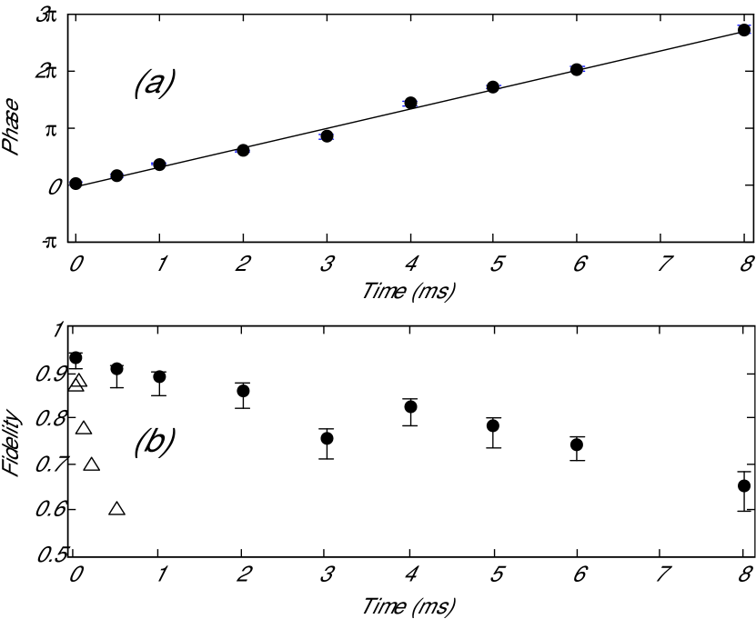
Figure 2: Time evolution of the state $\Psi_{+}=(|10\rangle+|01\rangle)\sqrt{2}$. A magnetic field gradient causes the relative phase between the $|10\rangle$ and the $|01\rangle$ parts to evolve linearly in time. Decoherence leads to a loss of fidelity. (a) Phase $\beta_{m}(t)$ for which the overlap $F_{m}=\max_{\beta}(\langle\Psi_{\beta}|\rho_{\Psi_{+}}(\tau)|\Psi_{\beta}\rangle)$ between $\rho_{\Psi_{+}}(\tau)$ and states of type $\Psi_{\beta}=(|10\rangle+\exp(i\beta)|01\rangle)\sqrt{2}$ is maximized. (b) Fidelity $F=\langle\Psi_{\beta_{L}}(t)|\rho(\tau)|\Psi_{\beta_{L}}(\tau)\rangle)$ of the measured density matrix $\rho(\tau)$ that nominally corresponds to the state $\Psi_{\beta_{L}}(\tau)=(|10\rangle+\exp(i\beta L)|01\rangle)\sqrt{2}$ (filled circles). The state $\Phi_{+}=(|11\rangle+|00\rangle)\sqrt{2}$ (triangles) is sensitive to fluctuations of the laser frequency and the magnetic field. Thus, its decay occurs on a much shorter time scale. Error bars account for quantum projection noise as well as systematic errors in the reconstruction process. They are derived from a Monte-Carlo simulation.

The phase changes linearly with time according to $\beta_{L}=\omega_{\beta}\tau$ with $\omega_{\beta}=(2\pi)170$ Hz, revealing the presence of a field gradient of $dB/dz=0.6$ G/cm in the direction of the ion string that transforms a $\Psi_{+}$ state into a $\Psi_{-}$ state within 3 ms and vice versagradient . The decay of the Bell state into a mixed state leads to a slow decline of the fidelity $F=\langle\Psi_{\beta_{L}}|\rho_{\Psi_{+}}(\tau)|\Psi_{\beta_{L}}\rangle$ over time which is shown in Fig. 2b. We find that the $\Psi_{\pm}$ states decay into a statistical mixture within 5 ms whereas the $\Phi_{\pm}$ states already decay after about 200 $\mu$s to a fidelity of $F=0.75$. That decay can also be seen by drawing the entanglement of formation and the smallest eigenvalue of the partial transpose as a function of time as shown in Fig. 3. In some measurements, we found even longer lifetimes of the $\Psi_{\pm}$ state approaching 20 ms.

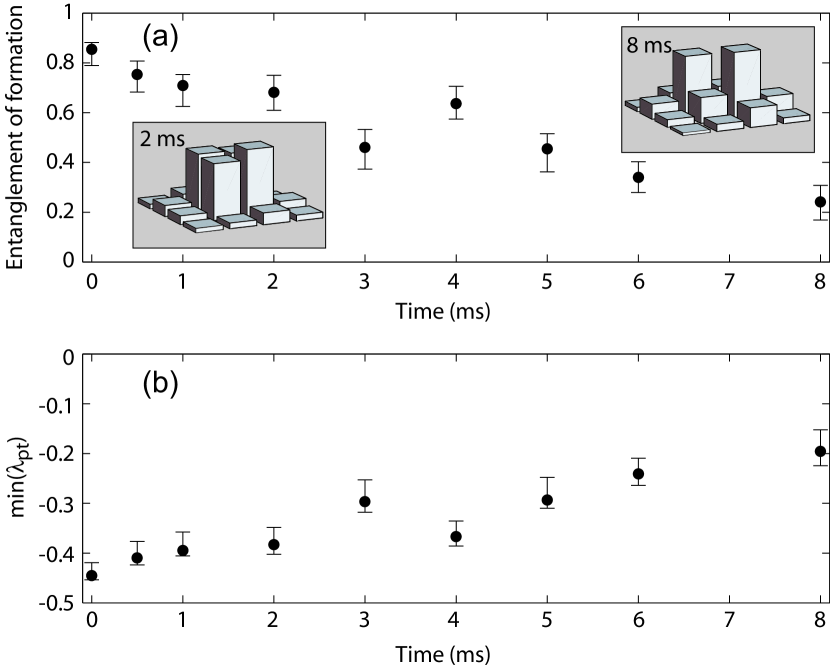
Figure 3: Decay of the Bell state $\Psi_{+}=(|10\rangle+|01\rangle)\sqrt{2}$ into a statistical mixture as a function of time. (a) Entanglement of formation and (b) smallest eigenvalue of the partial transpose of the density matrix. The insets show the magnitude of the density matrix elements measured after a time of 2 ms and 8 ms.

With the methods demonstrated above we have deterministically created all four Bell states. State tomography yielded the complete information about the two-qubit quantum states. In future, this tomographic procedure will provide an efficient tool for evaluating quantum gates and the effect of decoherence in multi-qubit systems. We gratefully acknowledge support by the European Commission (QUEST and QGATES networks), by the Austrian Science Fund (FWF), and by the Institut für Quanteninformation GmbH.

References

- (1) K. Vogel, H. Risken, Phys. Rev. A 40, 2847 (1989).
- (2) D. T. Smithey, M. Beck, M. G. Raymer, A. Faridani, Phys. Rev. Lett. 70, 1244 (1993).
- (3) T. J. Dunn, I. A. Walmsley, S. Mukamel, Phys. Rev. Lett. 74, 884 (1995).
- (4) D. Leibfried, D. M. Meekhof, B. E. King, C. Monroe, W. M. Itano, D. J. Wineland, Phys. Rev. Lett. 77, 4281 (1996).
- (5) Ch. Kurtsiefer, T. Pfau, J. Mlynek, Nature 386, 150 (1997).
- (6) I. L. Chuang, N. Gershenfeld, M. G. Kubinec, D. Leung, Proc. R. Soc. London A 454, 447 (1998).
- (7) A. G. White, D. F. V. James, P. H. Eberhard, P. G. Kwiat, Phys. Rev. Lett 83, 3103-3107 (1999).
- (8) A. G. White, D. F. V. James, W. J. Munro, P. G. Kwiat, Phys. Rev. A 65, 012301 (2001).
- (9) E. Hagley, X. Maître, G. Nogues, C. Wunderlich, M. Brune, J. M. Raimond, S. Haroche, Phys. Rev. Lett. 79, 1 (1997).
- (10) Q. A. Turchette, C. S. Wood, B. E. King, C. J. Myatt, D. Leibfried, W. M. Itano, C. Monroe, D. J. Wineland, Phys. Rev. Lett. 81, 3631 (1998).
- (11) D. Kielpinski, V. Meyer, M. A. Rowe, C. A. Sackett, W. M. Itano, C. Monroe, D. J. Wineland, Science 291, 1013 (2001).
- (12) F. Schmidt-Kaler et al., Nature 422, 408 (2003)
- (13) M. A. Nielsen, I. L. Chuang, Quantum Computation and Quantum Information (Cambridge Univ. Press, Cambridge, 2000).
- (14) Ch. Roos et al., Phys. Rev. Lett. 83, 4713 (1999).
- (15) F. Schmidt-Kaler et al., J. Phys. B: At. Mol. Opt. Phys. 36, 623 (2003).
- (16) H. Häffner et al., Phys. Rev. Lett. 90, 143602 (2003).
- (17) Note that and are eigenvectors of corresponding to the eigenvalues and , respectively.
- (18) U. Fano, Rev. Mod. Phys. 29, 74 (1957).
- (19) Z. Hradil, Phys. Rev. A 55, R1561 (1997).
- (20) K. Banaszek, G. M. D’Ariano, M. G. A. Paris, M. F. Sacchi, Phys. Rev. A 61, 010304 (1999).
- (21) D. F. V. James, P. G. Kwiat, W. J. Munro, A. G. White, Phys. Rev. A 64, 052312 (2001).
- (22) A. Peres, Phys. Rev. Lett. 77, 1413 (1996).
- (23) M. Horodecki, P. Horodecki, R. Horodecki, Phys. Lett. A 223, 1 (1996).
- (24) B. Efron, R. Tibshirani, Stat. Science 1, 54 (1986)
- (25) W. K. Wootters, Phys. Rev. Lett. 80, 2245 (1998).
- (26) The value of the field gradient was confirmed in an independent measurement.