Quasi-paraxial theory for coupled unstable cavities I: formal development

Abstract

We present a formal wave theory for the calculation of the spectrum and the eigenmodes for a certain class of ray-chaotic optical cavities introduced by A. Aiello, M. P. van Exter, and J. P. Woerdman [quant-ph/0307119].

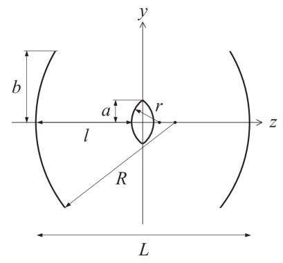
Figure 1: Schematic diagram of the cavity model. Two unstable cavities are coupled to form a single cavity which is globally stable for $L<2R$. The two sub-cavities are unstable for $l<R-r$ and stable for $R-r<l<R$.

In a previous paper Aiello et al. (2003), we presented a theoretical model for a composite optical cavity made of standard laser mirrors; the cavity consists of a suitable combination of stable and unstable cavities as shown in Fig. 1. By using numerical simulation we were able to demonstrate that such a cavity displays classical (ray) chaos, which may be either soft or hard, depending on the cavity configuration. In this paper we want to go a step further by addressing the behavior of the chaotic cavity in a wave regime (or, loosely speaking, in a “quantum” regime H. -J. Stöckmann (1999)). More precisely, in this paper we present a formal theory for two coupled unstable cavities. We show that it is possible to introduce an unitary coupling which accounts both for direct transmission and diffraction (which occurs from the edges of the convex mirrors in our cavity) by using a suitable scattering operator (see Eqs. (5-9) below).

A standard two-mirror stable resonator is a geometrically open system but because of its stability it is closed both from ray Hersch et al. (2000) and wave point of view. In other words, a typical gaussian-beam-like mode in such a resonator is confined both longitudinally (that is along the axis of the resonator) and transversally (that is along the two directions orthogonal to the axis) by the focussing action of the two mirrors. Because of this confinement a stable resonator has a discrete spectrum; in paraxial approximation this spectrum can be classified in a “longitudinal” part which depends only on the length of the cavity and in a “transversal” one which depends also from the radii of curvature of the two mirrors. Here we are interested mainly in the transversal part.
Efficient methods to calculate the spectrum and the eigenmodes of hard-edged unstable cavities were developed in the last 30 years; particularly notable is the asymptotic theory created by Horwitz Horwitz (1973) and Southwell Southwell (1986). However, in spite of this long hystory, surprising properties of these eigenmodes were discovered recently Karman and Woerdman (1998); Karman et al. (1999); Berry (2001); Berry et al. (2001). For instance, the Horowitz-Southwell theory has been exploited and slightly modified by Berry et. al. to investigate both the fractal nature of the cavity eigenmodes Berry et al. (2001) and the occurrence of the Petermann excess-noise factor Berry (2003). In this paper we apply Berry’s theory to our composite cavity, thus generalizing some of the results presented in Berry et al. (2001). From a mathematical point of view, the main difference between the theory for a conventional unstable cavity and our composite system, is that in the former case the operator which accounts for the modes propagation inside the unstable cavity is not unitary because of the losses from the edges of the smallest mirror. As we shall show later, in our case the two round-trip operators describing the mode propagation in the two half cavities shown in Fig. 1 remain non-unitary but the operator describing the motion in the overall cavity is unitary because the whole cavity is stable ($L<2R$).

In this paper we restrict our attention to two-dimensional cavities with one-dimensional mirrors (strip resonators). Following Berry Berry (2003) it is convenient to introduce from the beginning a “quantum-like” vector-space notation writing the modes of the field as kets in a linear space defined by the propagation operator $\hat{K}$ whose coordinate representation is given by the Huygens’ integral in the Fresnel approximation Siegman (1996). Within this formalism, the transversal mode profile $u(y)$ calculated in an arbitrary plane $z=$ const. can be considered as the coordinate representation of a field state $|u\rangle$ depending on the longitudinal coordinate $z$ which is considered as a parameter (exactly as the time in the Scrödinger equation):

$$\langle y|u\rangle\equiv u(y).$$ (1)

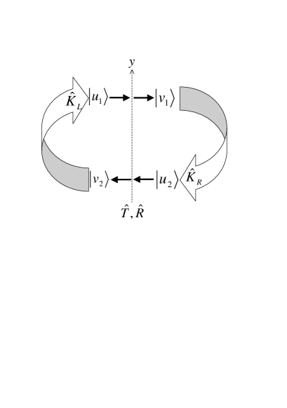
Figure 2: Logical scheme of the propagation process and of the coupling between the two sub-cavities. The dashed line represent the plane $z=0$ where the bi-convex mirror is located. $\hat{K}_{L}$, $\hat{K}_{R}$ are the operators describing the field propagation in the left and right side of the whole cavity while $\hat{T}$ and $\hat{R}$ describe the coupling between the two sub-cavities.

In order to describe the dynamics of each sub-cavity and the coupling between them, we introduce a set of four fields $u_{1},u_{2}$ and $v_{1},v_{2}$ defined in the reference plane $z=0$ following the scheme illustrated in Fig. 2. Then the propagation in the left and right side of the whole cavity can be described by introducing the operators $\hat{K}_{L}$ and $\hat{K}_{R}$ respectively:

$$\begin{array}[]{lcl}|u_{1}\rangle&=&e^{-i\frac{4\pi l_{1}}{\lambda}}\hat{K}_{L}|v_{2}\rangle,\\ |u_{2}\rangle&=&e^{-i\frac{4\pi l_{3}}{\lambda}}\hat{K}_{R}|v_{1}\rangle.\end{array}$$ (2)

At this point the two sub-cavities are still uncoupled. In Eq. (2) $\hat{K}_{L}=\hat{K}(l_{1})$, $\hat{K}_{R}=\hat{K}(l_{3})$, where $l_{1}$ and $l_{3}$ are the lengths of the left and right cavity respectively and the coordinate representation of the paraxial propagator is Siegman (1996)

$$\langle y|\hat{K}(l)|y^{\prime}\rangle=\sqrt{\frac{i}{B\lambda}}\exp\left[-i\frac{\pi}{B\lambda}\left(A{y^{\prime}}^{2}-2yy^{\prime}+Dy^{2}\right)\right].$$ (3)

The three coefficients $A,D,B$ are the corresponding elements of the following $ABCD$ matrix:

$$\mathbf{M}(l)=\left(\begin{array}[]{cc}1-\frac{2l}{R}&2l(1-\frac{l}{R})\\ \frac{2}{R}&1-\frac{2l}{R}\end{array}\right),$$ (4)

where $A=D$.

In order to describe the coupling between the two half cavities we introduce the four scattering operators $\hat{S}_{ij}$ $(i,j=1,2)$

$$\begin{array}[]{lcl}|v_{1}\rangle&=&\hat{S}_{11}|u_{1}\rangle+\hat{S}_{12}|u_{2}\rangle,\\ |v_{2}\rangle&=&\hat{S}_{21}|u_{1}\rangle+\hat{S}_{22}|u_{2}\rangle,\end{array}$$ (5)

where the diagonal operators $\hat{S}_{ii}$ describe the transmission of the field above the central mirror ($|y|>a$) while the off-diagonal operators $\hat{S}_{ij}$ $(i\neq j)$ describe the reflection on the central mirror ($|y|<a$). We require that the coupling between the two half cavities is unitary by imposing:

$$\langle u_{1}|u_{1}\rangle+\langle u_{2}|u_{2}\rangle=\langle v_{1}|v_{1}\rangle+\langle v_{2}|v_{2}\rangle,$$ (6)

from which it follows that:

$$\sum_{j=1}^{2}\hat{S}^{\dagger}_{ij}\hat{S}_{jk}=\hat{1}\delta_{ik},\qquad(i,j,k=1,2),$$ (7)

where $\delta_{ik}$ is the Kroneker tensor. Since the bi-convex optical element in the center of our cavity (see Fig. 1) is invariant with respect to the symmetry $z\rightarrow-z$, we can assume that the coupling is the same going from left to right and viceversa, and put:

$$\hat{S}_{11}=\hat{S}_{22}\equiv\hat{T},\qquad\hat{S}_{12}=\hat{S}_{21}\equiv\hat{R},$$ (8)

from which it follows that the unitarity conditions Eq. (7) become:

$$\begin{array}[]{ccc}\hat{T}^{\dagger}\hat{T}+\hat{R}^{\dagger}\hat{R}&=&1,\\ \hat{T}^{\dagger}\hat{R}+\hat{R}^{\dagger}\hat{T}&=&0.\end{array}$$ (9)

Before investigating the consequences of these relations we collect the four fields $u_{1},u_{2}$ and $v_{1},v_{2}$ in doublets

$$\{u_{1},u_{2}\}\rightarrow\left(\begin{array}[]{c}|u_{1}\rangle\\ |u_{2}\rangle\end{array}\right),\qquad\{v_{1},v_{2}\}\rightarrow\left(\begin{array}[]{c}|v_{1}\rangle\\ |v_{2}\rangle\end{array}\right),$$ (10)

which represent the incoming and outgoing fields in the plane $z=0$ respectively. Alternatively is possible to relate the fields in the left side of the cavity $\{u_{1},v_{2}\}$ with the fields on the right side $\{v_{1},u_{2}\}$ by introducing a set of four transmission operators that are related in a simple way to the scattering operators Spreeuw et al. (1992). However, we prefer to use the scattering formalism. Now we can rearrange the previous Eqs.(2-5) as

$$\begin{array}[]{ccc}\left(\begin{array}[]{c}|u_{1}\rangle\\ |u_{2}\rangle\end{array}\right)&=&\left(\begin{array}[]{cc}0&e^{-i\frac{4\pi l_{1}}{\lambda}}\hat{K}_{L}\\ e^{-i\frac{4\pi l_{3}}{\lambda}}\hat{K}_{R}&0\end{array}\right)\left(\begin{array}[]{c}|v_{1}\rangle\\ |v_{2}\rangle\end{array}\right),\end{array}$$ (11)

and

$$\begin{array}[]{ccc}\left(\begin{array}[]{c}|v_{1}\rangle\\ |v_{2}\rangle\end{array}\right)&=&\left(\begin{array}[]{cc}\hat{T}&\hat{R}\\ \hat{R}&\hat{T}\\ \end{array}\right)\left(\begin{array}[]{c}|u_{1}\rangle\\ |u_{2}\rangle\end{array}\right),\end{array}$$ (12)

respectively. Inserting Eq. (12) in Eq. (11) we obtain, after a few straightforward algebraic manipulation, and assuming the simpler case $l_{1}=l_{3}\equiv l\Rightarrow\hat{K}_{R}=\hat{K}_{L}\equiv\hat{K}$, the eigenvalue equation for the modes of the cavity:

$$\begin{array}[]{ccc}\left(\begin{array}[]{cc}\hat{R}\hat{K}-\gamma\hat{1}&\hat{T}\hat{K}\\ \hat{T}\hat{K}&\hat{R}\hat{K}-\gamma\hat{1}\end{array}\right)\left(\begin{array}[]{c}|v_{1}\rangle\\ |v_{2}\rangle\end{array}\right)&=&0,\end{array}$$ (13)

where we defined the eigenvalue $\gamma$ as: $\gamma=\exp(i\frac{4\pi l}{\lambda})$. By inspecting Eq. (13) we can easily recognize that the product $\hat{R}\hat{K}\equiv\hat{K}_{RT}$ is the well known round-trip propagator Berry (2003) for a single sub-cavity. Moreover we notice that when $\hat{T}=0$ we get two independent eigenvalue equations for the two unstable sub-cavities; in this case $\hat{K}_{RT}$ is not longer unitary and $|\gamma|<1$. With Eq. (13) we have achieved the goal of this paper. This equation can either be solved numerically by diagonalizing the matrix in Eq. (13) or by applying asymptotic methods Berry et al. (2001).
In order to write Eq. (13) in coordinate representation is necessary to write down the explicit form for the transmission $\hat{T}$ and the reflection $\hat{R}$ operators. To this end we first notice that the paraxial propagator which accounts for the reflection by a convex mirror has the following coordinate representation:

$$\langle y|\hat{r}|y^{\prime}\rangle=\exp\left(-\frac{2\pi i}{r\lambda}y^{2}\right)\delta(y-y^{\prime}),$$ (14)

where $r$ is the radius of the convex mirror Siegman (1996). Since the reflection operator is a mathematical representation of the bi-convex mirror whose transverse dimension is $2a$, its coordinate representation must be limited to the region $|y|\leq a$. Analogously it is easy to understand that the transmission operator can only exists in the region $|y|>a$. These physical considerations make it natural to try the following expressions for the transmission and reflection operators:

$$\begin{array}[]{lcl}\langle y|\hat{T}|y^{\prime}\rangle&=&\delta(y-y^{\prime})\Theta(|y|-a),\\ \langle y|\hat{R}|y^{\prime}\rangle&=&\delta(y-y^{\prime})\Theta(a-|y|)\exp\left(-\frac{2\pi i}{r\lambda}y^{2}\right).\end{array}$$ (15)

It is easy to check, by straightforward calculation, that choosing this form for the $\hat{R}$ and $\hat{T}$ operators, Eqs. (9) are automatically satisfied because of the following properties of the $\Theta$ functions:

$$\begin{array}[]{rcl}\Theta(|y|-a)+\Theta(a-|y|)&=&1,\\ \Theta(|y|-a)\Theta(a-|y|)&=&0.\end{array}$$ (16)

In conclusion, we have derived the equations for a pair of coupled unstable cavities. We obtained an eigenvalue equation (13) which can be solved in straightforward way to get the spectrum and the eigenmodes of the whole cavity. The theory in the present form involves some not well defined quantities (as products of distribution functions) which are justified only on a physical basis.

This project is part of the program of FOM and is also supported by the EU under the IST-ATESIT contract.

I Appendix

In this appendix we give some details about practical calculations. We start rewriting Eq. (13) as

$$\begin{array}[]{rcl}\gamma v_{1}(y)&=&\langle y|\hat{R}\hat{K}|v_{1}\rangle+\langle y|\hat{T}\hat{K}|v_{2}\rangle,\\ \\ \gamma v_{2}(y)&=&\langle y|\hat{T}\hat{K}|v_{1}\rangle+\langle y|\hat{R}\hat{K}|v_{2}\rangle.\end{array}$$ (17)

For simplicity we define $\hat{R}\hat{K}\equiv\hat{\rho}$ and $\hat{T}\hat{K}\equiv\hat{\tau}$ and write explicitly Eq. (17) as:

$$\begin{array}[]{rcl}\gamma v_{1}(y)&=&\displaystyle{\int dy^{\prime}\rho(y,y^{\prime})v_{1}(y^{\prime})+\int dy^{\prime}\tau(y,y^{\prime})v_{2}(y^{\prime})},\\ \\ \gamma v_{2}(y)&=&\displaystyle{\int dy^{\prime}\tau(y,y^{\prime})v_{1}(y^{\prime})+\int dy^{\prime}\rho(y,y^{\prime})v_{2}(y^{\prime})},\end{array}$$ (18)

where we have defined $\rho(y,y^{\prime})\equiv\langle y|\hat{\rho}|y^{\prime}\rangle$ and $\tau(y,y^{\prime})\equiv\langle y|\hat{\tau}|y^{\prime}\rangle$. For a symmetrical cavity with $l_{1}=l_{3}$ and we look for a solution such that $v_{1}(y)=v_{2}(y)$, therfore Eqs. (18) reduce to a single equation

$$\begin{array}[]{rcl}\gamma v_{1}(y)&=&\displaystyle{\int dy^{\prime}\left[\rho(y,y^{\prime})+\tau(y,y^{\prime})\right]v_{1}(y^{\prime})},\\ \\ &=&\displaystyle{\left[\Theta(a-|y|)\xi(y)+\Theta(|y|-a)\right]\int dy^{\prime}K(y,y^{\prime})v_{1}(y^{\prime})},\end{array}$$ (19)

where we have defined $\xi(y)\equiv\exp\left(-\frac{2\pi i}{r\lambda}y^{2}\right)$. Here $K(y,y^{\prime})$ is the propagator from a round-trip inside one unstable sub-cavity without accounting for the reflection on the convex mirror. Instead the product $\xi(y)K(y,y^{\prime})\equiv K_{RT}(y,y^{\prime})$ gives us the propagator for a complete round-trip. For computational reasons is more convenient to work with $K_{RT}(y,y^{\prime})$ instead of $K(y,y^{\prime})$ therefore, exploiting the fact that $|\xi(y)|^{2}=1$ we rewrite Eq. (19) as

$$\gamma v_{1}(y)=\displaystyle{\left[\Theta(a-|y|)+\Theta(|y|-a)\xi^{*}(y)\right]\int dy^{\prime}K_{RT}(y,y^{\prime})v_{1}(y^{\prime})}.$$ (20)

After scaling all lengths with $a$, Eq. (20)can be written as

$$\gamma g(y)=\displaystyle{\sqrt{\frac{it}{\pi}}\left[\Theta(1-|y|)+\Theta(|y|-1)\xi^{*}(y)\right]\int_{-\infty}^{\infty}e^{-it\left(x-y/M\right)^{2}}g(x)}dx,$$ (21)

where, following Horwitz Horwitz (1973), we have defined:

$$\begin{array}[]{rcl}M&=&\frac{\left[\sqrt{(l+r)(R-l)}+\sqrt{l(R-r-l)}\right]^{2}}{rR},\\ F&=&\frac{a^{2}}{2l\lambda(1-l/R)},\\ t&=&\pi MF,\\ \gamma&=&\gamma M^{-1/2},\\ g(y)&=&e^{i\pi F(M-M^{-1})/2y^{2}}v(y).\end{array}$$ (22)

The magnification $M$ can be also written in term of $m=(A+D)/2$, the half of the trace of the $ABCD$ matrix, as $M=m+\sqrt{m^{2}-1}$. In practice we have to calculate the asymptotic form of the following three integrals:

$$\begin{array}[]{rcl}I_{1}&=&\displaystyle{\int_{1}^{\infty}e^{-it\left(x-y/M\right)^{2}}g(x)dx},\\ \\ I_{2}&=&\displaystyle{\int_{-1}^{1}e^{-it\left(x-y/M\right)^{2}}g(x)dx},\\ \\ I_{3}&=&\displaystyle{\int_{-\infty}^{-1}e^{-it\left(x-y/M\right)^{2}}g(x)dx}.\end{array}$$ (23)

The value $x=y/M$ (with $M>1$) for which the phase is stationary can be inside or outside the domain of integration depending on the value of $y$ as illustrated in the following table:

Table 1: The real axis $(-\infty<y<\infty)$ has been divided in five subsets. For each of them the letters Y/N indicate if the stationary point is contained/not contained within the domain of integration of the integrals $I_{1},I_{2}$ and $I_{3}$.

	$-\infty<y<-M$	$-M<y<-1$	$-1<y<1$	$1<y<M$	$M<y<\infty$
$I_{1}$	N	N	N	N	Y
$I_{2}$	N	Y	Y	Y	N
$I_{3}$	Y	N	N	N	N

References

Aiello et al. (2003)
A. Aiello,
M. P. van Exter,
and J. P.
Woerdman, quant-ph/0307119
(2003), submitted to Phys. Rev. Lett.
H. -J. Stöckmann (1999)
H. -J. Stöckmann,
Quantum Chaos, An Introduction
(Cambridge University Press, 1999),
1st ed.
Hersch et al. (2000)
J. S. Hersch,
M. R. Haggerty,
and E. J.
Heller, Phys. Rev. E
62, 4873 (2000).
Horwitz (1973)
P. Horwitz, J.
Opt. Soc. Am. 63, 1528
(1973).
Southwell (1986)
W. H. Southwell,
J. Opt. Soc. Am. A 3,
1885 (1986).
Karman and Woerdman (1998)
G. P. Karman and
J. P. Woerdman,
Opt. Lett. 23,
1909 (1998).
Karman et al. (1999)
G. P. Karman,
G. S. McDonald,
G. H. C. New,
and J. P.
Woerdman, Nature
402, 138 (1999).
Berry (2001)
M. Berry, Opt.
Commun. 200, 321
(2001).
Berry et al. (2001)
M. Berry,
C. Storm, and
W. van Saarloos,
Opt. Commun. 197,
393 (2001).
Berry (2003)
M. Berry, J.
Mod. Optics 50, 63
(2003).
Siegman (1996)
A. E. Siegman,
Lasers (University Science
Books, Mill Valley, CA, 1996).
Spreeuw et al. (1992)
R. J. C. Spreeuw,
M. W. Beijersbergen,
and J. P.
Woerdman, Phys. Rev. A
45, 1213 (1992).