Collective vs local measurements in qubit mixed state estimation

Abstract

We discuss the problem of estimating a qubit mixed state. We give the optimal estimation that can be inferred from any given set of measurements. For collective measurements and for a large number, $N$, of copies, we show that the error in the estimation goes as $1/N$. For local measurements, we focus on the simpler case of states lying on the equatorial plane of the Bloch sphere. We show that the error using plain tomography goes as $1/N^{1/4}$, while our approach leads to an error proportional to $1/N^{3/4}$.

I Introduction

Knowing the state of a system is of paramount importance in quantum information. Quantum measurements provide only a partial knowledge of a state. Such a state, can only be reasonably reconstructed if a large number, $N$, of identically prepared copies of the system is available. Since the seminal work of Holevo holevo there has been a lot of research on this subject. Most of the quantitative analysis have mainly focused on pure states, for which the optimal strategies mp ; jones ; pure-states ; us-product ; us-local have been identified. They give the ultimate limits that can be achieved in state reconstruction. However, they involve collective measurements that, although very interesting from the theoretical point of view, are very resource consuming and very difficult to implement in a lab.

In the real world pure states are very scarce and so mixed state estimation is not just an academic issue. For instance, it is important to estimate the purity of a state, since this parameter often determines its utility to perform quantum information tasks. In quantum tomography, a quorum of local observables is measured on a (large) number of copies of a state $\rho$. From the relative frequencies of the outcomes, one then obtains an approximation or guess $\rho_{g}$ to the signal state $\rho$. However, the statistical deviations often yield unphysical states, e.g. ${\rm tr}\,{\rho_{g}}>1$. In this case, one can either discard the results or use a maximum likelihood data analysis likelihood . Using this analysis one infers the physical state that provides the closest theoretical probabilities to the observed frequencies. Many variants of these techniques can be found in the literature tomography ; likelihood , but there is a notorious lack of quantitative results (see though vidal ; density ).

The large numbers law ensures that with an infinite number of copies ($N\to\infty$) and infinite measurements the state could be exactly reconstructed by any sensible method. In practice, however, one has access only to limited resources and the crucial issue is to quantify the quality of the reconstruction procedure. This is the question we address here. We focus on qubit states and use the fidelity as figure of merit. We obtain the best estimate for any given measurement and compute the analytical expressions of the average fidelity for both collective and local (von Neumann) measurements in the asymptotic limit (large $N$).

II Bures Metric

The estimation procedure goes as follows. After we have measured on the $N$ copies of the system, some result is obtained, which we symbolically denote by $x$. Note that $x$ stands for both a single outcome of a collective measurement or a list of $N$ outcomes (one for each individual measurement) in local schemes. Based on $x$, an estimate for $\rho$ can be guessed, $\rho_{g}(x)$. The fidelity is defined as bures

$$f={\rm tr}\,\sqrt{{\rho_{g}^{1/2}(x)}\;\rho\;{\rho_{g}^{1/2}(x)}}.$$ (1)

It determines the maximum distinguishability between $\rho$ and $\rho_{g}(x)$ that can be achieved by any measurement fuchs . For qubits, Eq. 1 reads

$$f(\vec{r},\vec{R}(x))=\frac{1+\vec{r}\cdot\vec{R}(x)+\sqrt{1-r^{2}}\sqrt{1-R(x)^{2}}}{2}.$$ (2)

Here $r=|\vec{r}|$ and $R=|\vec{R}|$, where $\vec{r}$ and $\vec{R}(x)$ are the Bloch vectors of the states $\rho$ and $\rho_{g}(x)$ respectively [$\rho=(1+\vec{r}\cdot\vec{\sigma})/2$; $\vec{\sigma}=(\sigma_{x},\sigma_{y},\sigma_{z})$ are the standard Pauli matrices].

The fidelity can be viewed as a “distance” between two density matrices. The corresponding metric is usually known as Bures metric. From the infinitesimal “distance” $f(\vec{r},\vec{r}+d\vec{r})$ it is easy to obtain the volume element (normalized to unity: $\int\,d\rho=1$)

$$d\rho=\frac{2}{\pi}\frac{r^{2}dr}{\sqrt{1-r^{2}}}dn,\quad dn=\frac{\sin\theta d\theta d\phi}{4\pi},$$ (3)

where $dn$ is the invariant measure in the two-sphere. Eq. 3 is the natural uniform probability distribution function, or the a priori probability distribution for a completely unknown qubit state $\rho$. For our discussion below, we will also need $d\rho$ when the density matrices are known to lie in a great circle of the Bloch sphere. It reads

$$d\rho=\frac{1}{2\pi}\frac{rdr}{\sqrt{1-r^{2}}}d\theta.$$ (4)

Although in Section IV we use (3) and (4), our main results in the following section are independent of any particular choice of the a priori distribution.

III Fidelity and Optimal Guess

The average fidelity, hereafter fidelity in short, is the mean value of (1) over the a priori distribution and over all possible outcomes $x$,

$$F=\sum_{x}\int d\rho\,f(\vec{r},\vec{R}(x))p(x|\vec{r}),$$ (5)

where $p(x|\vec{r})$ is the conditional probability of obtaining outcome $x$ if the signal state has Bloch vector $\vec{r}$. These probabilities are determined by the expectation values of positive operators $O(x)$, such that $\sum_{x}O(x)=\mathbb{I}$, i.e., $p(x|\vec{r})={\rm tr}\,[O(x)\rho]$. Our aim is to maximize (5).

For a given measurement scheme, $\{O(x)\}$, there always exists an optimal guess, as we now show. We first introduce the four dimensional Euclidean vector

$$\mathbf{r}=(\sqrt{1-r^{2}},\vec{r}).$$ (6)

Note that $\mathbf{r}\cdot\mathbf{r}^{\prime}=\sqrt{1-r^{2}}\sqrt{1-r^{\prime 2}}+\vec{r}\cdot\vec{r}\,^{\prime}$ and $|\mathbf{r}|=\sqrt{\mathbf{r}\cdot\mathbf{r}}=1$. With this, the average fidelity reads

$$F=\sum_{x}\int d\rho\,\frac{1+\mathbf{r}\cdot\mathbf{R}(x)}{2}p(x|\vec{r}).$$ (7)

A straightforward use of the Schwarz inequality gives an upper bound of $F$ that is saturated with the choice

$$\mathbf{R}(x)=\frac{\mathbf{V}(x)}{|\mathbf{V}(x)|};\quad\mathbf{V}(x)=\int d\rho\,\mathbf{r}\,p(x|\vec{r}).$$ (8)

Using (8), the maximum fidelity is

$$F=\frac{1}{2}\left(1+\sum_{x}|\mathbf{V}(x)|\right).$$ (9)

Since the guess (8) satisfies $|\mathbf{R}(x)|=1$ and its first component is non-negative, it always gives a physical state. In fact, for any set of measurements and any a priori distribution, (8) is the best state that can be inferred and (9) is the maximum fidelity.

As the number of copies of the system becomes asymptotically large, any reasonable estimation scheme leads to a perfect reconstruction of the state, i.e, $F\to 1$. For a large, but finite $N$, the relevant issue is knowing the rate at which the perfect estimation limit is attained. For pure states, it is well known that the best collective strategy yields $F\sim 1-1/N$ ($F=1-1/(4N)$ for states on the equator of the Bloch sphere) mp . It has also been shown recently that this asymptotic limit can be achieved with local measurements us-local . For mixed states much less is known. Most of the pure state results can not be extrapolated to the mixed case, and some others may look counterintuitive at first sight. Although the space of mixed states seems to be larger, they are less distinguishable than pure states. The fidelity (2) has a minimum value $(1-r)/2$ which is never zero but for pure states ($r=1$). Thus the average fidelity could, in principle, be larger than that of pure states alone. Note that any estimated mixed state $\rho_{g}$ has some overlap with the signal state $\rho$. To be more concrete, imagine one does random guessing, without performing any measurement at all, i.e., $p(x|\vec{r})$ is uniform. Then, using Bures volume element (3), the average fidelity is $F_{\rm rand}=1/2+8/(9\pi^{2})$, which is larger than the random value ($F=1/2$) for pure states.

IV Results

IV.1 Collective measurements

As a first application of the results of the previous section, let us obtain the asymptotic behavior of the fidelity with the optimal collective measurement scheme. The main results are contained in vidal , where an optimal (and minimal) generalised measurement was obtained for qubit density matrices and generic isotropic probability distributions. However no definite form for this distribution was assumed and no explicit results were obtained. Our approach enables us to cast the expressions in vidal in a more transparent way as well as to simplify some of the derivations there. The optimal measurement is represented by a set of positive operators and conditional probabilities that can be labelled by two indices $x=(k,\vec{m})$. The discrete index $k$ labels the representations of the symmetric space spanned by $\{\rho^{\otimes N}\}$ onto which the positive operators of the measurement project, whereas the unit vector $\vec{m}$ labels a continuous set of outcomes in the two-sphere comentari . We have

$$p(k,\vec{m}|\vec{r})=c_{k}\left(\frac{1-r^{2}}{4}\right)^{N/2-k}\left(\frac{1+\vec{r}\cdot\vec{m}}{2}\right)^{2k},$$ (10)

where

$$c_{k}=\left(\begin{array}[]{c}N\\ N/2+k\end{array}\right)\frac{(2k+1)^{2}}{N/2+k+1}.$$ (11)

From (8) and (9) we obtain

$$F=\frac{1}{2}+\frac{1}{2}\sum_{k}\int dm\,|\mathbf{V}(k,\vec{m})|.$$ (12)

The sum in (12) runs from $k=0$ ($k=1/2)$ for $N$ even (odd) to $k=N/2$. Taking advantage of the rotational invariance, the integrals in (12) can be evaluated exactly. The computation of the asymptotic limit is rather lengthy and will not be reproduced here prep . The final result is

$$F=1-\left(\frac{3}{4}+\frac{4}{3\pi}\right)\frac{1}{N}+\cdots\ .$$ (13)

Note that this fidelity is only slightly worse than that of pure states: $3/4+4/(3\pi)=1.17\gtrsim 1$.

The expression (13) also gives us important information about the optimal fidelity when the a priori probability distribution corresponds to states known to lie in the equator plane of the Bloch sphere (4). Since in this situation we have more information about the states, the fidelity cannot be worse than (13), i.e. the error, defined as $E=1-F$, must satisfy $E\leq\xi/N$, where $\xi$ is a constant.

IV.2 Local measurements

Let us now tackle the problem of reconstructing a qubit state $\rho$ from local measurements. The analytical expressions turn out te be rather difficult to obtain and for simplicity only the case of states that are known to lie on the equator plane of the Bloch sphere (4) will be considered in this note. This is a non trivial case that can be relevant for quantum optics (e.g., for polarization states of photons). We will only sketch our main results. The techniques we have used are essentially contained in us-product ; us-local . Full details of the calculations will be presented elsewhere prep .

Consider $N=2{\mathscr{N}}$ copies of the state $\rho$. Quantum state tomography tells us that von Neumann measurements along two fixed orthogonal directions, $x$ and $y$, are sufficient to reconstruct the state. After the measurements, we obtain a set of outcomes $+1$ and $-1$ with relative frequencies $\alpha_{i}$ and $1-\alpha_{i}$, respectively ($i=x,y$). This occurs with probability

$$p(\vec{\alpha}|\vec{r})=\prod_{i}\left(\begin{array}[]{c}{\mathscr{N}}\\ {\mathscr{N}}\alpha_{i}\end{array}\right)\left(\frac{1+r_{i}}{2}\right)^{{\mathscr{N}}\alpha_{i}}\!\!\left(\frac{1-r_{i}}{2}\right)^{{\mathscr{N}}(1-\alpha_{i})}\kern-20.00003pt.$$ (14)

In quantum tomography the guess is given by

$$\mathbf{R}_{\rm T}(\vec{\alpha})=(\sqrt{1-R^{2}},R\cos\gamma,R\sin\gamma),$$ (15)

$$R\cos\gamma=2\alpha_{x}-1,\ \ \ \ \ R\sin\gamma=2\alpha_{y}-1.$$

In many instances, however, the statistical fluctuations produce an unphysical guess (the square root term becomes imaginary). If one discards these cases, the asymptotic behavior of the fidelity can be shown to be: $F=1-\xi_{\rm T}/N^{1/4}+\cdots$, where $\xi_{\rm T}$ is a constant. Although plain tomography yields a perfect reconstruction of the state in the asymptotic limit, it is much worse than the optimal collective scheme (note the power 1/4 of $N$ as compared to the power 1 in Eq. 13). One may suspect that the culprit of this behavior is the number of copies discarded, but we now show that it is not entirely so.

Within the maximum likelihood framework likelihood all available data is used. If $R\leq 1$, the guess is the tomographic one: $\mathbf{R}_{\rm ML}=\mathbf{R}_{\rm T}$ (see Eq. 15), and

$$\mathbf{R}_{\rm ML}=\left(0,\cos(\Phi),\sin(\Phi)\right)$$ (16)

if $R>1$, where $\Phi$ is the solution of the equation $\cos(2\Phi)=R\cos(\gamma+\Phi)$. In the asymptotic limit one can expand this equation as a power series in $(R-1)$, $\Phi=\gamma-(R-1)\cot 2\gamma+\cdots$. In fact only the first term is necessary for our calculation. After some effort one gets

$$F=1-\frac{\xi_{\rm ML}}{N^{3/4}}+\cdots;\quad\xi_{\rm ML}=\frac{\Gamma(1/4)^{3}}{2^{5/4}9\pi^{2}}\simeq 0.2256.$$ (17)

Notice the significant increase in the rate at which the fidelity approaches unity as compared to plain tomography.

Finally, we have computed the fidelity for the optimal guess (9). Here again, all available data is used to produce a reconstruction of the state. In Fig. 1 we compare the optimal guess and maximum likelihood methods for up to $N=20$ copies of a state. It is clear that the optimal guess strategy always performs better. We have also obtained the asymptotic limit. The fidelity reads in this case

$$F=1-\frac{\xi_{\rm O}}{N^{3/4}}+\cdots;\quad\xi_{\rm O}\simeq 0.1708,$$ (18)

where $\xi_{\rm O}$ can be computed analytically (see appendix). Notice that this fidelity approaches unity at a rate similar to the maximum likelihood one (17), but the coefficient of the first correction is lower ($\xi_{\rm O}<\xi_{\rm ML}$), as it should. The most important parameter is the exponent of the $1/N$ term in (18). It shows that, there is a gap in the quality of the reconstruction process between fixed local measurements and optimal collective schemes (recall Eq. 13). One may argue that we have not exploited classical communication, i.e, we have not designed each individual measurement according to the outcomes of the previous ones. We have also explored this possibility numerically and observed that the fidelity is almost identical to that obtained from the optimal guess with measurements along two fixed orthogonal directions. Therefore, we are led to conjecture that an error rate $E\sim 1/N^{3/4}$ is the lowest that can be achieved using any local scheme.

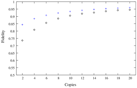
Figure 1: Average fidelities in terms of the number of copies. The diamonds (crosses) correspond to the maximum likelihood (optimal) guess.

V Conclusions

We have obtained the optimal reconstruction of a general qubit state for any given set of measurements and have illustrated our results in some interesting cases. We have computed the asymptotic expression of the fidelity for the optimal collective scheme. For local measurements we have considered the simpler but important case of states lying on the equator plane of the Bloch sphere. We have shown that the performance of plain tomography is very poor, with an error that goes as $E\sim 1/N^{1/4}$ for large $N$. We have shown that maximum likelihood does provide a much better estimation: $E\sim 1/N^{3/4}$. Using the same data, the optimal guess analysis gives the best reconstruction of the signal state. Despite this improvement, the asymptotic behavior of the fidelity does not saturate the optimal collective bound. This is in contrast to pure state estimation, where local measurements can perform optimally in the asymptotic regime. Although we have mainly focussed on measurements along fixed orthogonal directions, we have also analysed the most general local strategy, in which one is entitled to change these directions after each individual measurement. Our results strongly suggest that for mixed states the asymptotic behavior of the optimal collective schemes cannot be attained by any local strategy.

Appendix A

The $\xi_{\rm O}$ constant in (18) is the sum of three terms that can be written as

$$\xi_{\rm O} = \frac{\Gamma(1/4)^{2}}{48\pi}(4b_{1}+b_{2}-\sqrt{2}b_{3});$$

$$b_{1} = \int_{0}^{\infty}dx\left(\frac{e^{x}}{x^{3/4}{\rm Im}[K_{1/4}(-x)]}+\frac{\sqrt{2}}{\sqrt{\pi}x^{1/4}}\right),$$

$$b_{2} = \int_{0}^{\infty}dx\frac{e^{x}[{\rm erfc}(\sqrt{2x})-4]{\rm erfc}(\sqrt{2x})}{x^{3/4}{\rm Im}[K_{1/4}(-x)]},$$

$$b_{3} = \int_{0}^{\infty}dx\frac{e^{x}{\rm erfc}^{2}(\sqrt{2x})}{x^{3/4}K_{1/4}(x)},$$

where $K_{\nu}$ and ${\rm erfc}$ are the modified Bessel function and complementary error function respectively abramowitz . The integrals can be evaluated numerically: $b_{1}=0.197241$, $b_{2}=1.61451$ and $b_{3}=0.31400$. With these numbers we have $\xi_{\rm O}\simeq 0.17083$.

References

- (1) A.S. Holevo, Probabilistic and Statiscal Aspects of Quantum Theory (North Holland, Amsterdam, 1982).
- (2) S. Massar and S. Popescu, Phys. Rev. Lett. 74, 1259 (1995); R. Derka, V. Buzek and A. K. Ekert, Phys. Rev. Lett. 80, 1571 (1998).
- (3) K. R. W. Jones, Phys. Rev. A 50, 3682 (1994).
- (4) J. I. Latorre, P. Pascual and R. Tarrach, Phys. Rev. Lett. 81, 1351 (1998); N. Gisin and S. Popescu, Phys. Rev. Lett. 83, 432 (1999); E. Bagan et al., Phys. Rev. Lett. 85, 5230 (2000); ibid. Phys. Rev. A 63, 052309 (2001); D. G. Fischer, S. H. Kienle and M. Freyberger, Phys. Rev. A 61, 032306 (2000); R. D. Gill and S. Massar, Phys. Rev. A 61, 042312 (2000); A. Peres and P. F. Scudo, Phys. Rev. Lett. 86, 4160 (2001); Th. Hannemann et al., Phys. Rev. A 65, 050303 (2002).
- (5) E. Bagan, M. Baig and R. Munoz-Tapia, Phys. Rev. A 64, 022305 (2001).
- (6) E. Bagan, M. Baig and R. Munoz-Tapia, Phys. Rev. Lett. 89, 277904 (2002).
- (7) Z. Hradil, Phys. Rev. A 55, 1561 (1997); K. Banaszek, et al., Phys. Rev. A 61, 010304 (2000).
- (8) G. M. D’Ariano and M. G. A. Paris, Phys. Rev. A 60, 518 (1999); D. F. V. James, et al., Phys. Rev. A 64, 052312 (2001); R. T. Thew, et al., Phys. Rev. A 66, 012303 (2002); G. M. D’Ariano, L. Maccone and M. Paini, J. Opt B 5, 77 (2003).
- (9) G. Vidal, et al., Phys. Rev. A 60, 126 (1999).
- (10) J. I. Cirac, A. K. Ekert and C. Macchiavello, Phys. Rev. Lett. 82, 4344 (1999); D. G. Fischer and M. Freyberger, Phys. Lett. A 273, 293 (2000); M. Keyl and R. F. Werner, Phys. Rev. A 64, 052311 (2001).
- (11) M. Huebner, Phys. Lett. A 163, 239 (1992); R. Josza, J. Mod. Opt. 41, 2315 (1994).
- (12) C. A. Fuchs, PhD Dissertation (University of New Mexico, 1995); quant-ph/9601020.
- (13) In Ref. vidal the authors use a discrete set of directions instead of the continuous set considered here.
- (14) E. Bagan, et al., in preparation.
- (15) M. Abramowitz and I.A. Stegun, Handbook of Mathematical Functions (Dover, New York 1970).