Nonrelativistic system of interacting particles in the model
of the noncommutative operators of coordinates and momenta
of different particles

Abstract

It is shown that the Schrödinger equation for a system of interacting particles whose Compton wavelengths are of the same order of magnitude as the system size is contradictory and is not strictly nonrelativistic, because it is based on the implicit assumption that the velocity of propagation of interactions is finite. In the framework of the model of the noncommutative operators of coordinates and momenta of different particles, the equation for a wave function which has no above-mentioned drawbacks is deduced. The significant differences from solutions of the nonrelativistic Schrödinger equation for large values of the interaction constant are found, and the comparison of analogous results for hydrogenlike atoms with experimental data is carried out.

I Introduction

All the known relativistic and quasirelativistic quantum descriptions of systems of interacting particles are constructed, as a rule, so that they are reduced to the well-known Schrödinger equation in the nonrelativistic limit. Therefore, there arises the question about the correctness of the Schrödinger equation in the description of a nonrelativistic system of particles interacting with one another through various potentials with any admissible parameters. The present work is devoted to the study of this question.

As known, the Compton wavelength $\hbar/mc$ Landau and Peierls (1931) is the limit, up to which one can comprehensively introduce the notion of coordinate for a nonrelativistic particle with mass $m$. Here, $\hbar=h/2\pi$, where $h$ is the Planck constant, and $c$ is the velocity of light in vacuum. That is, the coordinate of a nonrelativistic particle cannot be measured with higher accuracy than its Compton wavelength:

$$\Delta x>\frac{\hbar}{mc}\;.$$ (1)

Therefore, for the system of two nonrelativistic interacting particles with masses $m_{1}$ and $m_{2}$, respectively, the mean distance between the particles cannot be measured with higher accuracy than

$$\Delta_{12}=\sqrt{\left(\frac{\hbar}{m_{1}c}\right)^{2}+\left(\frac{\hbar}{m_{2}c}\right)^{2}}=\frac{\hbar}{\mu c}\sqrt{1-\frac{2\mu}{M}}\;,$$ (2)

where $\mu$ is the reduced mass of the system, $\mu^{-1}=m_{1}^{-1}+m_{2}^{-1}$, and $M=m_{1}+m_{2}$ is the total mass of the system of two particles. Here, we assume that $\hbar/m_{1}c$ ($\hbar/m_{2}c$) is the root-mean-square deviation upon the measurement of the independent coordinate of the first (second) particle. Then $\Delta_{12}$ in Eq. (2) is the root-mean-square deviation upon the measurement of the distance between the particles J.R.Taylor (1982). Therefore, there is no sense in the saying about the mean distance between the particles which is less than $\Delta_{12}$.

On the other hand, the mean distance between particles in the Schrödinger theory of a hydrogenlike atom in the ground state is equal to

$$\left\langle\left|{\bf r}_{2}-{\bf r}_{1}\right|\right\rangle=\frac{3}{2}\,\frac{\hbar}{\mu c}\,\frac{1}{\alpha Z}\;.$$ (3)

Here, $Z$ is the atomic nucleus charge and $\alpha$ is the fine structure constant. It is clear that we can get $\left\langle\left|{\bf r}_{2}-{\bf r}_{1}\right|\right\rangle\ll\hbar/{\mu c}$ (for a hydrogenlike atom, $\mu/M\ll 1$) for sufficiently large $Z$. In this case, we do not consider the question about the rightfulness of the nonrelativistic approximation.

These contradictions indicate that the Schrödinger equation for a system of nonrelativistic interacting particles is not fully correct because the mean distance between particles can be significantly less than $\Delta_{12}$.

The probabilistic treatment of the squared modulus of a wave function is possible only under the assumption that the measurements of coordinates or momenta of different particles do not basically perturb each other even in the presence of any interaction forces between particles W.Pauli (1958). This means that the operators of coordinates or momenta of two particles commute with each other. In addition, the operators of coordinates and momenta of different particles commute with one another in the Schrödinger theory, which means the absence of mutual interferences upon the measurements of a coordinate of one particle and a momentum of the other. The last assertion is true if the time of measurement of the coordinate of a particle is considerably less than the time of propagation of a light signal across the distance equal to the system size or, which is the same, if the Compton wavelengths of particles are considerably less than the system size. Therefore, the Schrödinger equation works very well in atomic physics and solid state physics. However, the application of the Schrödinger equation to atomic nuclei seems to be not exactly correct, because the Compton wavelength of a nucleon is comparable with the size of an atomic nucleus itself. In addition, the strict nonrelativistic formulation requires to consider the interaction propagation velocity to be infinite, which forces us to consider the operators of coordinates and momenta of different particles to be noncommutative with one another Kuzmenko (2000). This noncommutativity leads to the existence of a critical value of the interaction constant for the Coulomb potential such that the ground state of a hydrogenlike atom cannot exist for its larger values. Work Kuzmenko (2000) is phenomenological to a certain extent, because the choice of the parameter inherent in the theory is ambiguous. The present work develops the ideas put forth in the previous one Kuzmenko (2000). We propose to choose the parameter inherent in our theory in such a way that the least average distance between particles in the ground state in the Coulomb field be equal to $\Delta_{12}$. For other potentials, especially short-range ones of the Yukawa or Hulthén type, the use of this parameter leads to average distances being at least $\Delta_{12}$.

II Two-body problem in the framework of the model of the noncommutative operators of coordinates and momenta of different particles.

As known, the classical equations of motion for a particle of mass $m$ in the external field $V\left({\bf r}\right)$ are derived from the Hamilton function

$$H\left({\bf r},{\bf p}\right)=\frac{{\bf p}^{2}}{2m}+V\left({\bf r}\right)$$ (4)

which depends on the coordinates of a particle ${\bf r}$ and the corresponding momentum ${\bf p}$. The total energy of the system is

$$E=H\left({\bf r},{\bf p}\right)\;.$$ (5)

With this classical system, we associate a quantum system whose dynamical state is represented by a wave function $\Psi\left({\bf r},t\right)$ defined in the configurational space. The wave equation is constructed by the formal substitution of the quantities $E$, ${\bf r}$, and ${\bf p}$ on both sides of relation (5) by the relevant operators Messiah (1961)

$$E\to\hat{E}=i\hbar\frac{\partial}{\partial t}\;,$$ (6)

$${\bf r}\to{\bf\hat{r}}={\bf r}\;,$$ (7)

$${\bf p}\to{\bf\hat{p}}=-i\hbar\bm{\nabla}\;.$$ (8)

It is implied that the results of action of both sides of equality (5) considered as operators on $\Psi\left({\bf r},t\right)$ are identical. In view of this fact, we get the nonrelativistic Schrödinger equation for a particle in the external field $V\left({\bf r}\right)$:

$$i\hbar\frac{\partial}{\partial t}\Psi\left({\bf r},t\right)=\left[-\frac{\hbar^{2}}{2m}\Delta+V\left({\bf r}\right)\right]\Psi\left({\bf r},t\right)\;.$$ (9)

We emphasize that the operators ${\bf\hat{r}}$ and ${\bf\hat{p}}$ in Eqs. (7) and (8) are written in the configurational space and ${\bf r}$ is the vector of a position of the particle in a rectangular coordinate system.

The operators of coordinate and momentum are noncommutative,

$$\left[{\hat{x}\,,\,\hat{p}_{x}}\right]=i\hbar\;,\quad\left[{\hat{y}\,,\,\hat{p}_{y}}\right]=i\hbar\;,\quad\left[{\hat{z}\,,\,\hat{p}_{z}}\right]=i\hbar\;,$$ (10)

which yields the Heisenberg uncertainty relations

$$\Delta x\Delta p_{x}\geq\hbar/2\;,\;\Delta y\Delta p_{y}\geq\hbar/2\;,\;\Delta z\Delta p_{z}\geq\hbar/2\;,$$ (11)

where the quantities $\Delta x$, $\Delta p_{x}$, $\Delta y$, $\Delta p_{y}$, $\Delta z$, and $\Delta p_{z}$ are directly connected with relevant measurements and are the root-mean-square deviations from the mean value. For example, for the coordinate $x$, we have

$$\Delta x=\sqrt{\langle\hat{x}^{2}\rangle-\langle\hat{x}\rangle^{2}}\;,$$ (12)

where $\langle\hat{A}\rangle$ is the mean value of the operator $\hat{A}$ on the wave function $\Psi\left({\bf r},t\right)$.

Relations (11) state that a particle cannot be in the states where its coordinate and momentum take simultaneously quite definite, exact values. In addition, quantum theory states that the unpredictable and uncontrolled disturbance undergone by the physical system in the process of measurement is always finite and such that the Heisenberg uncertainty relations (11) are satisfied Messiah (1961). Hence, none experiment can realize the simultaneous exact measurement of the coordinate and momentum of a particle. For example, the measurement of the coordinate $x$ with accuracy $\Delta x$ in the well-known experiment with the use of a Heisenberg microscope is accompanied by the uncontrolled momentum transfer to the particle which is characterized by the uncertainty

$$\Delta p_{x}\approx\frac{\hbar}{2\Delta x}\;.$$ (13)

In this case, the limits of exactness in the determination of a position are always set by optical resolving power conditioned by the effects of diffraction according to classical wave optics.

If the system size is such that the characteristic time of flight with the velocity of light across the system exceeds considerably the duration of the process of measurement of a position $\Delta t$, then we may say that the process of measurement of the coordinate of a particle with accuracy $\Delta x$ is accompanied by a blow against the particle with the force

$$F_{x}\approx\frac{\Delta p_{x}}{\Delta t}\approx\frac{\hbar c}{2(\Delta x)^{2}}\;.$$ (14)

Here, we assume that the momentum transferred to the particle under measurement of its coordinate is of the same order as the root-mean-square deviation $\Delta p_{x}$.

In the measurement of the momentum of a particle with accuracy $\Delta p_{x}$, it undergoes a blow with the force

$$F_{x}\approx\frac{2c}{\hbar}(\Delta p_{x})^{2}\;.$$ (15)

Analogously to Eq. (9), one can deduce the Schrödinger nonrelativistic equation for a system of two interacting particles whose Hamilton function is

$$H=\frac{{\bf p}_{1}^{2}}{2m_{1}}+\frac{{\bf p}_{2}^{2}}{2m_{2}}+V\left(\left|{\bf r}_{2}-{\bf r}_{1}\right|\right)\;.$$ (16)

Here, ${\bf r}_{1}$ and ${\bf r}_{2}$ are the Cartesian coordinates of a position of two particles with masses $m_{1}$ and $m_{2}$, ${\bf p}_{1}$ and ${\bf p}_{2}$ are their relevant momenta, and the potential energy depends only on the distance between the particles.

With this classical system, we associate a quantum system whose dynamical state is represented by a wave function $\Psi({\bf r}_{1},{\bf r}_{2},t)$ defined in the configurational space. The wave equation is derived by means of the formal substitution of the quantities $E$, ${\bf r}_{1}$, ${\bf r}_{2}$, ${\bf p}_{1}$, and ${\bf p}_{2}$ on both sides of the relation analogous to Eq. (5) by the corresponding operators:

$$E\to\hat{E}=i\hbar\frac{\partial}{\partial t}\;,$$ (17)

$${\bf r}_{1}\to{\bf\hat{r}}_{1}={\bf r}_{1}\;,$$ (18)

$${\bf r}_{2}\to{\bf\hat{r}}_{2}={\bf r}_{2}\;,$$ (19)

$${\bf p}_{1}\to{\bf\hat{p}}_{1}=-i\hbar\bm{\nabla}_{1}\;,$$ (20)

$${\bf p}_{2}\to{\bf\hat{p}}_{2}=-i\hbar\bm{\nabla}_{2}\;.$$ (21)

Then the well-known Schrödinger nonrelativistic equation for a system of two interacting particles reads

$$i\hbar\frac{\partial}{\partial t}\Psi=\left[-\frac{\hbar^{2}}{2m_{1}}\Delta_{1}-\frac{\hbar^{2}}{2m_{2}}\Delta_{2}+V\left(\left|{\bf r}_{2}-{\bf r}_{1}\right|\right)\right]\Psi\;.$$ (22)

The operators ${\bf\hat{r}}_{1}$, ${\bf\hat{r}}_{2}$, ${\bf\hat{p}}_{1}$, and ${\bf\hat{p}}_{2}$ satisfy the following commutation relations:

$$\left[{\hat{x}_{k},\hat{p}_{kx}}\right]=i\hbar,\,\left[{\hat{y}_{k},\hat{p}_{ky}}\right]=i\hbar,\,\left[{\hat{z}_{k},\hat{p}_{kz}}\right]=i\hbar,\;k=1,2.$$ (23)

All the rest possible commutation relations are zero including such as

$$\left[{\hat{x}_{k},\hat{p}_{lx}}\right]=0,\,\left[{\hat{y}_{k},\hat{p}_{ly}}\right]=0,\,\left[{\hat{z}_{k},\hat{p}_{lz}}\right]=0,\;(k\neq l).$$ (24)

Equalities (24) are based on the assumption that the measurements of coordinates and momenta of different particles do not basically disturb one another even in the presence of any interaction forces between particles W.Pauli (1958). That is, it is assumed that a change of the force action of one particle on the other one induced by the measurement of the coordinate of the former is propagated with finite velocity.

Thus, in the derivation of the Schrödinger nonrelativistic equation for a system of two particles, one uses, on the one hand, a Hamilton nonrelativistic classical function and, on the other hand, the implicit assumption that the interaction propagation velocity is finite.

Within the fully nonrelativistic quantum theory, we must consider the interaction propagation velocity to be infinite, which forces us to refuse the fulfillment of the commutation relations (24). From this viewpoint, we will consider that, under the measurement of the coordinate of the first particle, the uncontrolled momentum transfer to not only this particle, but to the whole system, occurs since the particles are bound with each other by the interaction potential whose propagation velocity is infinite. Therefore, it is natural to require that the commutator of the coordinate operator of the first particle and the operator of the total momentum of the system be equal to $i\hbar$:

$$\left[{\hat{x}_{1}\,,\,\hat{P}_{x}}\right]=i\hbar\,,\,\left[{\hat{y}_{1}\,,\,\hat{P}_{y}}\right]=i\hbar\,,\,\left[{\hat{z}_{1}\,,\,\hat{P}_{z}}\right]=i\hbar\;.$$ (25)

Here, ${\bf\hat{P}}={\bf\hat{p}}_{1}+{\bf\hat{p}}_{2}$ is the operator of the total momentum of the system. The same should be true for the second particle:

$$\left[{\hat{x}_{2}\,,\,\hat{P}_{x}}\right]=i\hbar\,,\,\left[{\hat{y}_{2}\,,\,\hat{P}_{y}}\right]=i\hbar\,,\,\left[{\hat{z}_{2}\,,\,\hat{P}_{z}}\right]=i\hbar\;.$$ (26)

We note that relations (25) and (26) are satisfied also for the Schrödinger nonrelativistic equation, and just they allow one to construct the operator of coordinates of the center of masses of the system whose commutator with the operator of the total momentum of the system is equal to $i\hbar$. On the contrary, the fulfillment of relations (23) is not obligatory for a system of interacting particles, and we intend to refuse it.

Of course, under the measurement of the coordinate of some particle with accuracy $\Delta x$, the system undergoes a blow with the force $\approx{\hbar c}/{2(\Delta x)^{2}}$. For example, the measurement of the coordinate of a nonrelativistic electron with the maximally possible accuracy of order of the Compton wavelength $\hbar/m_{e}c=3.86\times 10^{-11}\mathop{\rm cm}$ is accompanied by a blow with the force $F_{e}\approx 6.62\times 10^{9}\mathop{\rm MeV}/\mathop{\rm cm}$. For a proton, the Compton wavelength is about $2.10\times 10^{-14}\mathop{\rm cm}$, and the blow force equals $F_{p}\approx 2.24\times 10^{16}\mathop{\rm MeV}/\mathop{\rm cm}$. The mean interaction force between the particles in a hydrogen atom in the ground state $F_{H}\approx 1.03\times 10^{4}\mathop{\rm MeV}/\mathop{\rm cm}$, and $F_{D}\approx 4.50\times 10^{14}\mathop{\rm MeV}/\mathop{\rm cm}$ for a bound state of a deuterium nucleus. Therefore, we can neglect the interaction force between the particles in a hydrogen atom under the measurement of their coordinates because $F_{H}/F_{e}\approx 1.56\times 10^{-6}$ and consider the operators of coordinates and momenta of different particles to be commutative. But the situation is different in atomic nuclei, because the ratio of the interparticle interaction force to the blow force is $F_{D}/F_{p}\approx 0.02$.

In the general case, we take

$$\left[{\hat{x}_{1}\,,\,\hat{p}_{2x}}\right]=i\hbar\hat{\varepsilon}_{12}\;,$$ (27)

where $\hat{\varepsilon}_{12}$ is some dimensionless Hermitian operator. Then Eq. (25) yields that

$$\left[{\hat{x}_{1}\,,\,\hat{p}_{1x}}\right]=i\hbar(1-\hat{\varepsilon}_{12})\;.$$ (28)

Analogously, if

$$\left[{\hat{x}_{2}\,,\,\hat{p}_{1x}}\right]=i\hbar\hat{\varepsilon}_{21}\;,$$ (29)

then

$$\left[{\hat{x}_{2}\,,\,\hat{p}_{2x}}\right]=i\hbar(1-\hat{\varepsilon}_{21})\;.$$ (30)

The dimensionless Hermitian operators $\hat{\varepsilon}_{12}$ and $\hat{\varepsilon}_{21}$ depend in the general case on the interparticle interaction force ${\bf F}_{12}$ and on masses $m_{1}$ and $m_{2}$. The operators $\hat{\varepsilon}_{12}$ and $\hat{\varepsilon}_{21}$ cannot depend on the direction of the vector ${\bf F}_{12}$, because the commutation relations for the $x$, $y$, and $z$ components must be identical analogously to Eqs. (27)-(30), because the system has no distinguished directions and the independent variables are fully equivalent in a rectangular coordinate system. Therefore, the operators $\hat{\varepsilon}_{12}$ and $\hat{\varepsilon}_{21}$ are functions of the force modulus, i.e. of $\left|{\bf F}_{12}\right|$:

$$\hat{\varepsilon}_{12}\equiv\hat{\varepsilon}_{12}\left(m_{1},m_{2},\left|{\bf F}_{12}\right|\right),\,\hat{\varepsilon}_{21}\equiv\hat{\varepsilon}_{21}\left(m_{1},m_{2},\left|{\bf F}_{12}\right|\right).$$ (31)

For the operators $\hat{x}_{1}$ and $\hat{p}_{2x}$ which do not commute with each other, the uncertainty relation looks de Broglie (1982) as

$$\Delta x_{1}\Delta p_{2x}\geq\frac{\hbar}{2}\left|{\langle\hat{\varepsilon}_{12}\rangle}\right|\;,$$ (32)

where $\langle\hat{\varepsilon}_{12}\rangle$ is the quantum-mechanical mean in the state $\Psi({\bf r}_{1},{\bf r}_{2},t)$. In the general case, the right-hand side of the uncertainty relation (32) takes different values for every quantum state, which hampers significantly the derivation of a wave equation. The problem can be considerably simplified if the operator $\hat{\varepsilon}_{12}$ in Eq. (27) is substituted by the modulus of its quantum-mechanical mean $\left|{\left\langle{\hat{\varepsilon}_{12}}\right\rangle}\right|$ in the ground state of the system. In this case, the right-hand side of relation (32) takes the value which is maximum of all the possible ones, because the mean interparticle interaction force in the ground state is maximum and therefore the momentum transferred to the second particle under the measurement of the coordinate of the first one is maximum. It is worth noting that, in such a statement, the uncertainty relation (32) is not changed in the ground state of the system. A similar simplification can be made also for the operator $\hat{\varepsilon}_{21}$, which allows us to eventually deduce a nonrelativistic wave equation for a system of two particles.

The commutation relations for the operators of coordinates or momenta of different particles remain the same as in the Schrödinger theory,

$$\left[{\hat{x}_{1}\,,\,\hat{x}_{2}}\right]=0\;,\quad\left[{\hat{p}_{1x}\,,\,\hat{p}_{2x}}\right]=0\;,$$ (33)

which allows one to use these operators as independent variables.

Below, we write the commutation relations for all the operators of coordinates and momenta of the two-body problem:

$$\left[{\hat{x}_{1}\,,\,\hat{p}_{1x}}\right]=i\hbar(1-\varepsilon_{12})\;,$$ (34)

$$\left[{\hat{x}_{2}\,,\,\hat{p}_{2x}}\right]=i\hbar(1-\varepsilon_{21})\;,$$ (35)

$$\left[{\hat{x}_{1}\,,\,\hat{p}_{2x}}\right]=i\hbar\varepsilon_{12}\;,$$ (36)

$$\left[{\hat{x}_{2}\,,\,\hat{p}_{1x}}\right]=i\hbar\varepsilon_{21}\;,$$ (37)

$$\left[{\hat{x}_{1}\,,\,\hat{x}_{2}}\right]=0\;,$$ (38)

$$\left[{\hat{p}_{1x}\,,\,\hat{p}_{2x}}\right]=0\;.$$ (39)

Analogous relations hold for the $y$ and $z$ components. We recall that $\varepsilon_{12}$ and $\varepsilon_{21}$ are the moduli of the quantum-mechanical means of the operators $\hat{\varepsilon}_{12}$ and $\hat{\varepsilon}_{21}$ in the ground state $\Psi_{0}({\bf r}_{1},{\bf r}_{2},t)$ of the system:

$$\varepsilon_{12}=\left|\frac{\left\langle\Psi_{0}\right|\hat{\varepsilon}_{12}(m_{1},m_{2},\left|{\bf F}_{12}\right|)\left|\Psi_{0}\right\rangle}{\left\langle\Psi_{0}\left|\right.\Psi_{0}\right\rangle}\right|\;,$$ (40)

$$\varepsilon_{21}=\left|\frac{\left\langle\Psi_{0}\right|\hat{\varepsilon}_{21}(m_{1},m_{2},\left|{\bf F}_{12}\right|)\left|\Psi_{0}\right\rangle}{\left\langle\Psi_{0}\left|\right.\Psi_{0}\right\rangle}\right|\;.$$ (41)

We estimate now the quantities $\varepsilon_{12}$ and $\varepsilon_{21}$. We assume that the momentum transferred to a particle is of order of the root-mean-square deviation $\Delta p$. Then Eq. (34) and Eq. (36) yield

$$\Delta x_{1}\Delta p_{1x}\approx\frac{\hbar}{2}(1-\varepsilon_{12})\;,$$ (42)

$$\Delta x_{1}\Delta p_{2x}\approx\frac{\hbar}{2}\varepsilon_{12}\;.$$ (43)

Whence we get

$$\varepsilon_{12}=\frac{\Delta p_{2x}}{\Delta p_{1x}}\left(1+\frac{\Delta p_{2x}}{\Delta p_{1x}}\right)^{-1}\;.$$ (44)

Here, $\Delta p_{2x}$ is the momentum transferred to the second particle under the measurement of the coordinate of the first one, and $\Delta p_{1x}$ is the momentum transferred to the first particle under the measurement of its coordinate. We assume further that the coordinate of the first particle is measured with the highest possible accuracy, i.e., $\Delta x_{1}=\hbar/m_{1}c$. In this case, the momentum transferred to the second particle can be estimated as

$$\Delta p_{2x}=\left\langle\left|{\bf F}_{12}\right|\right\rangle\Delta t=\left\langle\left|{\bf F}_{12}\right|\right\rangle\frac{\Delta x_{1}}{c}=\left\langle\left|{\bf F}_{12}\right|\right\rangle\frac{\hbar}{m_{1}c^{2}}\;.$$ (45)

Here, $\left\langle\left|{\bf F}_{12}\right|\right\rangle$ is the mean value of the force in a given quantum state, $\Delta t$ is the duration of measurement of the coordinate of the first particle. We assume that the momentum transferred to the second particle, Eq. (45), is small. Then the momentum which will be transferred to the first particle can be estimated as

$$\Delta p_{1x}=\frac{\hbar}{2\Delta x_{1}}=\frac{m_{1}c}{2}$$ (46)

and $\Delta p_{2x}/{\Delta p_{1x}}$ can be written as

$$\frac{\Delta p_{2x}}{\Delta p_{1x}}=\xi\frac{m_{2}^{2}}{M^{2}}\;,$$ (47)

where $\xi=2\hbar\left\langle\left|{\bf F}_{12}\right|\right\rangle/{\mu^{2}c^{3}}$. In what follows, we assume that the functional dependence on the mean interaction force $\left\langle\left|{\bf F}_{12}\right|\right\rangle$ in Eq. (47) is preserved, and a more exact dependence on the masses of interacting particles is taken into account by the introduction of a constant $\Omega$ which will be defined by the requirement that the least mean distance between particles in the ground state of a hydrogenlike atom be equal to $\Delta_{12}$. By running ahead, we note that $\Omega$ depends only on the ratio $\mu/M$. Finally, we get the following expression for the noncommutativity parameter $\varepsilon_{12}$:

$$\varepsilon_{12}=\Omega\xi\frac{m_{2}^{2}}{M^{2}}\left(1+\Omega\xi\frac{m_{2}^{2}}{M^{2}}\right)^{-1}\;.$$ (48)

The noncommutativity parameter $\varepsilon_{21}$ can be derived analogously as

$$\varepsilon_{21}=\Omega\xi\frac{m_{1}^{2}}{M^{2}}\left(1+\Omega\xi\frac{m_{1}^{2}}{M^{2}}\right)^{-1}\;.$$ (49)

Now we can construct one of the possible representations for the operators of coordinates and momenta of a system of two particles:

$${\bf\hat{r}}_{1}={\bf r}_{1}\;,$$ (50)

$${\bf\hat{r}}_{2}={\bf r}_{2}\;,$$ (51)

$${\bf\hat{p}}_{1}=-i\hbar(1-\varepsilon_{12})\bm{\nabla}_{1}-i\hbar\varepsilon_{21}\bm{\nabla}_{2}\;,$$ (52)

$${\bf\hat{p}}_{2}=-i\hbar\varepsilon_{12}\bm{\nabla}_{1}-i\hbar(1-\varepsilon_{21})\bm{\nabla}_{2}\;.$$ (53)

It is easy to verify that operators (50)-(53) satisfy the commutation relations (34)-(39).

The operator of the total momentum of the system

$${\bf\hat{P}}={\bf\hat{p}}_{1}+{\bf\hat{p}}_{2}=-i\hbar\bm{\nabla}_{1}-i\hbar\bm{\nabla}_{2}\;.$$ (54)

By substituting the quantities in the Hamilton function (16) by operators (50)-(53), we get the nonrelativistic wave equation for a system of two particles as

$$i\hbar\frac{\partial}{\partial t}\Psi\left({\bf r}_{1},{\bf r}_{2},t\right)=H\Psi\left({\bf r}_{1},{\bf r}_{2},t\right)\;,$$ (55)

with the Hamiltonian of the system

$$H=-{A}_{1}\Delta_{1}-{A}_{2}\Delta_{2}-{A}_{12}(\bm{\nabla}_{1}\cdot\bm{\nabla}_{2})+V\left(\left|{\bf r}_{1}-{\bf r}_{2}\right|\right)\;,$$ (56)

where $A_{1}={\hbar^{2}}(1-\varepsilon_{12})^{2}/{2m_{1}}+{\hbar^{2}}\varepsilon_{12}^{2}/{2m_{2}}$, $A_{2}={\hbar^{2}}(1-\varepsilon_{21})^{2}/{2m_{2}}+{\hbar^{2}}\varepsilon_{21}^{2}/{2m_{1}}$, and $A_{12}={\hbar^{2}}\varepsilon_{21}(1-\varepsilon_{12})/m_{1}+{\hbar^{2}}\varepsilon_{12}(1-\varepsilon_{21})/m_{2}$.

Consider the Hamiltonian of an isolated system which does not depend on time, and therefore the energy of the system is the integral of motion. By using the substitution

$$\Psi=\psi\exp\left(-i\frac{E_{0}t}{\hbar}\right)\;,$$ (57)

where $\psi$ depends on coordinates of the configurational space but is independent of time, we get the equation for the stationary states of a system of two particles $H\psi=E_{0}\psi$. Here, $E_{0}$ is the total energy of the two-particle system. If we use the substitution of variables

$${\bf r}={\bf r}_{1}-{\bf r}_{2}\;,$$ (58)

$${\bf R}=\frac{m_{1}}{M}{{\bf r}_{1}}+\frac{m_{2}}{M}{{\bf r}_{2}}+\frac{m_{1}\varepsilon_{12}-m_{2}\varepsilon_{21}}{M\beta}\left({\bf r}_{1}-{\bf r}_{2}\right)\;,$$ (59)

the equation for the wave function admits the separation of variables after the substitution $\psi({\bf r},{\bf R})=\Phi({\bf R})\phi({\bf r})$. In this case, the Hamiltonian of the system takes the following form:

$$H=-\frac{\hbar^{2}}{2M}\Delta_{\bf R}-\frac{\hbar^{2}\beta^{2}}{2\mu}\Delta_{\bf r}+V\left(\left|{\bf r}\right|\right)\;.$$ (60)

Here, $\beta=1-\varepsilon_{12}-\varepsilon_{21}$. In this case, we get the quantum-mechanical description of two noninteracting fictitious particles, the first of which represents a free motion of a particle with mass equal to the sum of masses of the particles and with momentum equal to the total momentum of the system (${\bf\hat{P}}={\bf\hat{p}}_{1}+{\bf\hat{p}}_{2}=-i\hbar\bm{\nabla}_{1}-i\hbar\bm{\nabla}_{2}=-i\hbar\bm{\nabla}_{\bf R}$). The position of this particle is set by the vector ${\bf R}$ which does not define the coordinate of the center of masses in the general case, whereas this is true for the Schrödinger equation, but only in the case of identical particles. The second fictitious particle with mass $m=\mu\beta^{-2}$ moves in the field $V\left(\left|{\bf r}\right|\right)$ and represents the relative motion of two particles with energy $E$.

Since no external fields act on the system, its Hamiltonian must be invariant with respect to both a parallel translation of the coordinate system in space and a rotation of the coordinate axes. In addition, the equations of motion do not vary under a uniform and rectilinear motion of the system (the Galilei invariance).

The operator of the total momentum of the system ${\bf\hat{P}}={\bf\hat{p}}_{1}+{\bf\hat{p}}_{2}=-i\hbar\bm{\nabla}_{1}-i\hbar\bm{\nabla}_{2}$ is connected with the operator of the infinitesimal translation transforming the function $\Psi({\bf r}_{1},{\bf r}_{2})$ into $\Psi({\bf r}_{1}+\delta{\bf r},{\bf r}_{2}+\delta{\bf r})$,

$$1+\delta{\bf r}\cdot\sum\limits_{i=1}^{2}\bm{\nabla}_{i}=1+\frac{i}{\hbar}\delta{\bf r\cdot\hat{P}}\;,$$ (61)

and commutes with Hamiltonian (60),

$$\left[H\,,\,{\bf\hat{P}}\right]=0\;,$$ (62)

where $\delta{\bf r}$ is the vector of an infinitesimal parallel translation of all the radius-vectors of the particles by the same value, ${\bf r}_{i}\to{\bf r}_{i}+\delta{\bf r}$, and the operator of the total momentum looks as ${\bf\hat{P}}=-i\hbar\bm{\nabla}_{\bf R}$ in variables (58) and (59). Thus, three components of the total momentum are the integrals of motion, and the total momentum of the system of two particles is preserved.

By virtue of isotropy of the space, the Hamiltonian of a closed system must be invariant under a rotation of the whole system by an arbitrary angle around any axis. It suffices to require the fulfillment of this condition for any infinitesimal rotation whose vector $\delta\bm{\varphi}$ has the modulus equal to the rotation angle $\delta\varphi$ and is directed along the rotation axis. The operator of the infinitesimal rotation transforming the function $\Psi({\bf r}_{1},{\bf r}_{2})$ into $\Psi({\bf r}_{1}+[\delta\bm{\varphi}\times{\bf r}_{1}],\,{\bf r}_{2}+[\delta\bm{\varphi}\times{\bf r}_{2}])$ is connected with the operator of the total angular momentum of the system

$$1+\delta\bm{\varphi}\cdot\sum\limits_{i=1}^{2}\left[{\bf r}_{i}\times\bm{\nabla}_{i}\right]=1+\frac{i}{\hbar}\delta\bm{\varphi}\cdot{\bf\hat{L}}$$ (63)

and commutes with Hamiltonian (60) of the system. Thus, the total angular momentum ${\bf\hat{L}}=-i\hbar\sum\limits_{i=1}^{2}\left[{\bf r}_{i}\times\bm{\nabla}_{i}\right]=-i\hbar\left[{\bf r}\times\bm{\nabla}_{\bf r}\right]-i\hbar\left[{\bf R}\times\bm{\nabla}_{\bf R}\right]$ of the system of two particles is preserved.

It is important to note the following fact. By writing formally the operators ${\bf\hat{l}}_{1}=\left[{\bf\hat{r}}_{1}\times{\bf\hat{p}}_{1}\right]$ and ${\bf\hat{l}}_{2}=\left[{\bf\hat{r}}_{2}\times{\bf\hat{p}}_{2}\right]$ for each particle, we can easily prove that they and their sum are not angular momenta, because they do not satisfy the standard commutation relations intrinsic to the angular momentum:

$$\left[{\hat{L}_{x},\hat{L}_{y}}\right]=i\hbar\hat{L}_{z},\;\left[{\hat{L}_{y},\hat{L}_{z}}\right]=i\hbar\hat{L}_{x},\;\left[{\hat{L}_{z},\hat{L}_{x}}\right]=i\hbar\hat{L}_{y}\;.$$ (64)

However, from the operators ${\bf\hat{r}}_{i}$ and ${\bf\hat{p}}_{j}$, we can construct an operator which will possess the above-mentioned properties of the total angular momentum:

$${\bf\hat{L}}=\sum\limits_{i,j}{C_{ij}}\left[{\bf\hat{r}}_{i}\times{\bf\hat{p}}_{j}\right]=-i\hbar\sum\limits_{i=1}^{2}\left[{\bf r}_{i}\times\bm{\nabla}_{i}\right]\;.$$ (65)

For a system of two particles, the coefficients $C_{ij}$ read

$$C_{11}=(1-\varepsilon_{21})\beta^{-1}\;,$$ (66)

$$C_{22}=(1-\varepsilon_{12})\beta^{-1}\;,$$ (67)

$$C_{12}=-\varepsilon_{21}\beta^{-1}\;,$$ (68)

$$C_{21}=-\varepsilon_{12}\beta^{-1}\;.$$ (69)

We should like to emphasize that the noncommutativity parameters of the operators of coordinates and momenta of different particles, $\varepsilon_{12}$ and $\varepsilon_{21}$, depend on the mean value of the modulus of the interaction force between two particles in the ground state (i.e., on the distance between the particles). On the motion of two reference systems relatively each other with constant velocity ${\bf v}$, the operators ${\bf\hat{r}}_{i}$ and ${\bf\hat{p}}_{i}$ are transformed, respectively, into ${\bf\hat{r}}_{i}-{\bf v}t$ and ${\bf\hat{p}}_{i}-m_{i}{\bf v}$. Such a Galilei transformation of a system of particles is described by the operator Messiah (1961)

$$\hat{G}({\bf v},t)=\exp\left[{i{\bf v}(M{\bf\hat{R}}-{\bf\hat{P}}t)/\hbar}\right]\;,$$ (70)

where $M$ and ${\bf\hat{P}}$ are the mass and the operator of the total momentum of the system of two particles and ${\bf\hat{R}}$ is vector (59) of a position of the fictitious free particle. It is easy to show that the condition for the equation of motion (55) to be Galilei-invariant,

$$\hat{G}^{\dagger}({\bf v},t)\left[i\hbar\frac{\partial}{\partial t}-H\right]\hat{G}({\bf v},t)=\left[i\hbar\frac{\partial}{\partial t}-H\right]\;,$$ (71)

is satisfied for Hamiltonian (60).

For the wave function of relative motion of the particles, we get the following equation:

$$\left[-\frac{\hbar^{2}\beta^{2}}{2\mu}\Delta_{\bf r}+V\left(\left|{\bf r}\right|\right)\right]\phi\left({\bf r}\right)=E\phi\left({\bf r}\right)\;,$$ (72)

where

$$\beta=\frac{1-\Omega^{2}\xi^{2}\mu^{2}M^{-2}}{1+\Omega^{2}\xi^{2}\mu^{2}M^{-2}+\Omega\xi\left(1-2\mu/M\right)}\;,$$ (73)

$$\xi=\frac{2\hbar}{\mu^{2}c^{3}}\left\langle\phi_{0}\right.\left|\left|{\bf F}_{12}\right|\right|\left.\phi_{0}\right\rangle/\left\langle\phi_{0}\left|\phi_{0}\right.\right\rangle\;.$$ (74)

The total energy of the system is $E_{0}=E+E_{\bf R}$, where $E_{\bf R}$ is the energy of free motion of the first fictitious particle.

Similarly to the Schrödinger nonrelativistic theory, the wave function $\phi({\bf r})$ should be continuous together with its partial derivatives of the first order in the entire space. In addition, the wave function $\phi({\bf r})$ should be a bounded and one-valued function of its arguments.

Similarly to the Schrödinger theory for particles interacting through a centrally symmetric potential which depends only on the distance between particles, the wave function $\phi({\bf r})$ can be represented as

$$\phi({\bf r})=\frac{1}{r}\chi_{l}(r)Y_{lm}\left(\frac{\bf r}{r}\right)\;,$$ (75)

where $Y_{lm}\left({\bf n}\right)$ are the orthonormalized spherical functions. Then the function $\chi_{l}(r)$ satisfies the equation

$$\left[-\frac{\hbar^{2}\beta^{2}}{2\mu}\left(\frac{d^{2}}{dr^{2}}-\frac{l(l+1)}{r^{2}}\right)+V\left(r\right)\right]\chi_{l}(r)=E\chi_{l}(r)$$ (76)

which has solutions for a system of two interacting particles at definite values of the energy $E$.

The constant $\Omega$ can be determined by considering the ground state of the discrete spectrum of a hydrogenlike atom. Let two particles with masses $m_{1}$ (atomic nucleus) and $m_{2}$ (electron) be bound by the Coulomb potential $V(r)=-Ze^{2}/r$, where $Z$ is the atomic nucleus charge. The equation for bound states can be written as

$$\left[-\frac{\hbar^{2}\beta^{2}}{2\mu}\left(\frac{d^{2}}{dr^{2}}-\frac{l(l+1)}{r^{2}}\right)-\frac{Ze^{2}}{r}\right]\chi_{nl}(r)=E_{nl}\chi_{nl}(r)\;.$$ (77)

Here, we took into account that $m_{1}\gg m_{2}$ and then $\beta=(1+\Omega\xi_{0})^{-1}$ and wrote the index 0 to the parameter $\xi$ by emphasizing the fact that it is defined by the ground quantum state. Equation (77) is the equation for the radial functions of a hydrogenlike atom by the Schrödinger theory whose normed solutions are well known for bound states (see, e.g., Bethe and Salpeter (1957)):

$$\chi_{nl}(r)=N_{nl}\,r^{l+1}F\left(-n+l+1,2l+2,\frac{2Zr}{na_{0}\beta^{2}}\right)$$

$$\times\exp\left(-\frac{Zr}{na_{0}\beta^{2}}\right)\;,$$ (78)

where

$$N_{nl}=\frac{1}{(2l+1)!}\left[\frac{(n+l)!}{2n(n-l-1)!}\right]^{1/2}\left(\frac{2Z}{na_{0}\beta^{2}}\right)^{l+3/2}\;.$$ (79)

Here, $a_{0}=\hbar^{2}/\mu e^{2}$ is the Bohr radius and $F$ is a confluent hypergeometric function. The eigenvalues of the energy of bound states are

$$E_{nl}=-\frac{\mu c^{2}}{2}\frac{(\alpha Z)^{2}}{n^{2}}\left(1+\Omega\xi_{0}\right)^{2}\;.$$ (80)

Here, $l=0,1,\dots,n-1$ and $n=1,2,\dots,\infty$.

By substituting $\chi_{10}(r)$ into Eq. (74), we obtain the nonlinear equation for the determination of $\xi_{0}$:

$$\frac{\eta_{0}}{(1+\eta_{0})^{4}}=4\Omega(\alpha Z)^{3};\;\;\;\;\eta_{0}=\Omega\xi_{0}\;.$$ (81)

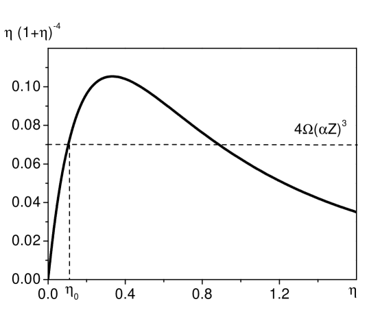
Figure 1: Graphical solution of Eq. (81) for $\eta_{0}$ at various values of the parameter $4\Omega(\alpha Z)^{3}$ for the ground state of a hydrogenlike atom.

The nonlinear equation (81) for $\eta_{0}$ has solutions under the condition $4\Omega(\alpha Z)^{3}\leq 27/256$, which is shown in Fig. 1. From two solutions, suitable is a solution which is positioned nearer to zero. The second solution should be omitted since it corresponds to the case where the binding energy increases with decrease in the parameter $\alpha Z$. For $4\Omega(\alpha Z)^{3}>27/256$, Eq. (81) has no solutions, which means the impossibility for a given bound state to exist. The critical value of the interaction constant $Z=Z_{C}$ is reached at $\eta_{0}=1/3$. In this case, the mean distance between particles attains the minimum value

$$\left\langle\left|{\bf r}_{2}-{\bf r}_{1}\right|\right\rangle=\frac{3}{2}\frac{\hbar}{\mu c}\frac{1}{\alpha Z_{C}}\frac{1}{(1+\eta_{0})^{2}}\;.$$ (82)

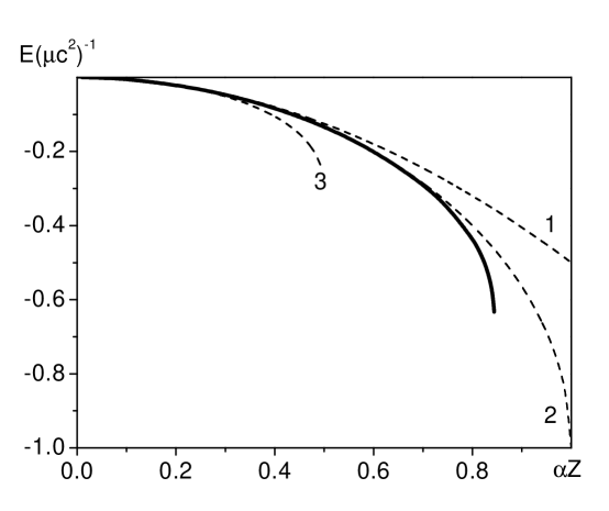
Figure 2: Binding energy of the ground state of a hydrogenlike atom vs the parameter $\alpha Z$. For the sake of comparison, we present the corresponding dependences according to the equations of Schrödinger (1), Dirac (2), and Klein-Gordon (3).

By requiring that this least value be equal to $\hbar/\mu c$, we determined the parameter $\Omega$ whose value is $32/729$. In this case, the critical value of $Z_{C}$ equals $115.6\;\;\left(\alpha Z_{C}=27/32\right)$. The binding energy for the ground state of a hydrogenlike atom, which is calculated by using the parameter $\Omega$ determined in such a way, is displayed in Fig. 2, where the analogous dependences of the binding energies within the Schrödinger, Dirac, and Klein-Gordon theories are also presented. As seen, the energy levels of the ground state are positioned below the Schrödinger levels and above those calculated by the Dirac theory in a rather wide interval of values of the interaction constant ($0<\alpha Z<0.685$). Excited states of a hydrogenlike atom are positioned below relevant Schrödinger levels.

The noncommutativity parameters of the operators of coordinates and momenta of different particles $\varepsilon_{12}$ and $\varepsilon_{21}$ for a hydrogenlike atom can be estimated as follows:

$$\varepsilon_{12}=\Omega\xi_{0}\frac{m_{2}^{2}}{M^{2}}=\eta_{0}\frac{m_{2}^{2}}{M^{2}}\;,$$ (83)

$$\varepsilon_{21}=\frac{\Omega\xi_{0}}{1+\Omega\xi_{0}}=\frac{\eta_{0}}{1+\eta_{0}}\;.$$ (84)

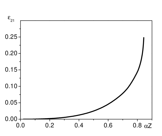
Figure 3: Dependence of the noncommutativity parameter $\varepsilon_{21}$ on the interaction constant for a hydrogenlike atom.

The last dependence is shown in Fig. 3. For a hydrogen atom, the noncommutativity parameters are $\varepsilon_{12}=2.0\times 10^{-14}$ and $\varepsilon_{21}=6.8\times 10^{-8}$.

Of significant interest is the comparison of the obtained results with the available experimental data and the consequences of the Schrödinger nonrelativistic theory because the high-precision experimental measurements of the energy levels of a hydrogen atom  Udem et al. (1997), light hydrogenlike atoms (see the review  Eides et al. (2001)), and heavy ions ${}^{92}U$ with one Stohlker et al. (2000) or several electrons Schweppe et al. (1991); Beiersdorfer et al. (1993) have been recently performed.

Table 1 presents the ground state energies of some hydrogenlike atoms together with experimental data and the results following from the Schrödinger equation. The experimental data for $Z=6-42$ and $Z=92$ are taken, respectively, from NIST Atomic Spectra Databases (http://physics.nist.gov) and Stohlker et al. (2000). The last two columns, in which the differences of the theoretical energy levels by Schrödinger and by Eq. (80) with experimental data are given, demonstrate the advantage of the proposed nonrelativistic quantum-mechanical method of description of hydrogenlike atoms at great interaction constants $\alpha Z$. Indeed, the difference between the theoretical and experimental values of the ground state energy of a hydrogenlike atom for middle values of $Z$ is approximately twice less than that by Schrödinger. The very good agreement with the experimental value of the ground state energy is obtained for hydrogenlike uranium, which corresponds to the region of intersection ($Z=94$) of the theoretical curve of the ground state energy versus $\alpha Z$ and the relevant curve (Fig. 2) for the Dirac equation. In the region of the critical value of the interaction constant ($Z=115$), the significant role is played by relativistic effects. Therefore, in this case, one should expect a worse agreement with experimental data. In addition, the consideration of relativistic effects can change the critical value of the interaction constant in the direction of its growth. Analogous conclusions can be drawn from Table 2 which gives the theoretical, experimental, and Schrödinger-equation-based values of the gap between levels 1s and 2s.

Table 1: Binding energy of the ground state $E$ (see Eq. (80)) for certain hydrogenlike atoms as compared to the experimental data $E_{\rm{EXP}}$ and those by the Schrödinger equation $E_{S}$. All values are given in $\mathop{\rm eV}$.

$Z$	$E$	$E_{\rm{EXP}}$	$E_{S}-E_{\rm{EXP}}$	$E-E_{\rm{EXP}}$
6	$-489.8193$	$-489.9933$	$0.1884$	$0.1740$
12	$-1959.682$	$-1962.665$	$3.445$	$2.983$
18	$-4411.759$	$-4426.224$	$17.980$	$14.465$
24	$-7851.73$	$-7894.80$	$57.92$	$43.07$
30	$-12290.62$	$-12388.93$	$143.81$	$98.31$
36	$-17746.88$	$-17936.21$	$303.23$	$189.33$
42	$-24248.77$	$-24572.23$	$571.79$	$323.46$
92	$-131726.$	$-131812.$	$16653.$	$86.$

Table 2: Gaps between levels 1s and 2s for certain hydrogenlike atoms calculated in this work $\Delta=E(2s)-E(1s)$ as compared to the experimental data $\Delta_{\rm{EXP}}$ and those by the Schrödinger equation $\Delta_{S}$. All values are given in $\mathop{\rm eV}$.

$Z$	$\Delta$	$\Delta_{\rm{EXP}}$	$\Delta_{\rm{EXP}}-\Delta_{S}$	$\Delta_{\rm{EXP}}-\Delta$
6	$367.3645$	$367.4774$	$0.1237$	$0.1129$
12	$1469.761$	$1471.729$	$2.314$	$1.968$
18	$3308.819$	$3318.338$	$12.155$	$9.519$
24	$5888.794$	$5916.929$	$39.270$	$28.135$
30	$9217.96$	$9281.538$	$97.696$	$63.578$
36	$13310.16$	$13431.01$	$206.28$	$120.85$
42	$18186.58$	$18389.67$	$389.34$	$203.09$

The constant $\Omega=32/729$ is derived under the condition $\mu/M\ll 1$. For another relation between the masses of interacting particles, it is necessary to use the complete expression for $\beta$ [ Eq. (73)] to derive the constant $\Omega$ from the condition that the minimum mean distance between particles reaches $\Delta_{12}$. This dependence is shown in Fig. 4. The good approximation of the dependence of $\Omega$ on $\mu/M$ is attained by the expression $\Omega=32(1-2\mu M^{-1})/729$ shown in Fig. 4 by the dotted line. This approximation is convenient for a quantum system composed of several particles with different masses. Of great interest is the situation with two identical particles. In this case, $\mu/M=0.25$, $\beta=\left(1-\Omega\xi_{0}/4\right)/\left(1+\Omega\xi_{0}/4\right)$, and $\Omega=0.0211547$.

For other interaction potentials between particles, we may take the parameter $\Omega$ which was derived for a hydrogenlike atom. We note that even the potentials with a singularity at zero (those of the Yukawa or Hulthén type) lead to the mean distance between particles which is at least $\Delta_{12}$ given by Eq. (2).

Below, we give the values of the Poisson quantum brackets proposed by Dirac Dirac (1958):

$$\left\{\hat{x}_{1}\,,\hat{p}_{1x}\right\}=1-\varepsilon_{12}\;,$$ (85)

$$\left\{\hat{x}_{2}\,,\hat{p}_{2x}\right\}=1-\varepsilon_{21}\;,$$ (86)

$$\left\{\hat{x}_{1}\,,\hat{p}_{2x}\right\}=\varepsilon_{12}\;,$$ (87)

$$\left\{\hat{x}_{2}\,,\hat{p}_{1x}\right\}=\varepsilon_{21}\;,$$ (88)

$$\left\{\hat{x}_{1}\,,\hat{x}_{2}\right\}=0\;,$$ (89)

$$\left\{\hat{p}_{1x}\,,\hat{p}_{2x}\right\}=0.$$ (90)

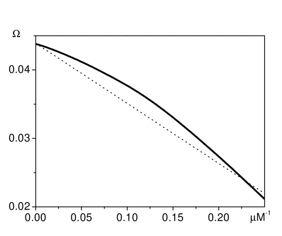
Figure 4: Parameter $\Omega$ vs $\mu/M$ in the two-body problem.

For $\varepsilon_{12},\varepsilon_{21}\to 0$, these brackets are transformed into the classical Poisson ones, i.e., we have the full analogy between classical mechanics and quantum one in this case. As seen in Fig. 3, $\varepsilon_{21}$ differs considerably from zero in the systems whose sizes are of order of the Compton wavelengths of the particles composing a system. In this case, the analogy with classical mechanics is absent.

III Nonrelativistic system of $N$ interacting particles

The above results can be easily generalized for a system consisting of $N$ particles which are bound with one another by two-particle forces.

Let the operators of coordinates and momenta of $N$ particles be ${\bf\hat{r}}_{1}$, ${\bf\hat{r}}_{2}$, $\dots$ , ${\bf\hat{r}}_{N}$, ${\bf\hat{p}}_{1}$, ${\bf\hat{p}}_{2}$, $\dots$ , ${\bf\hat{p}}_{N}$. We define the operator of the total momentum of the system as

$${\bf\hat{P}}=\sum\limits_{k=1}^{N}{\bf\hat{p}}_{k}\;.$$ (91)

Analogously to the two-particle problem, we require that the commutator of the coordinate operator of any particle with the operator of the total momentum of the system be equal to $i\hbar$:

$$\left[{\bf\hat{r}}_{i}\,,{\bf\hat{P}}\right]=i\hbar\;,\;\;\;i=1,2,\dots,N\;.$$ (92)

Then if

$$\left[{\bf\hat{r}}_{i}\,,{\bf\hat{p}}_{k}\right]=i\hbar\varepsilon_{ik}\;,\;\;\;i\neq k\;,$$ (93)

we get

$$\left[{\bf\hat{r}}_{i}\,,{\bf\hat{p}}_{i}\right]=i\hbar\left[1-\sum\limits_{k=1}^{N}\varepsilon_{ik}\right]\;,\;\;\;i=1,2,\dots,N\;.$$ (94)

Here, the noncommutativity parameter of the operators of coordinates and momenta of different particles $\varepsilon_{ik}$ equals zero for $i=k$ ($\varepsilon_{ii}=0$), which was made for the sake of convenience to write the further formulas. In addition,

$$\left[{\bf\hat{r}}_{i}\,,{\bf\hat{r}}_{k}\right]=0\;,\quad\left[{\bf\hat{p}}_{i}\,,{\bf\hat{p}}_{k}\right]=0\;.$$ (95)

One of the possible representations of the operators of coordinates and momenta of particles can be written as

$${\bf\hat{r}}_{i}={\bf r}_{i}\;,$$ (96)

$${\bf\hat{p}}_{i}=-i\hbar\left[1-\sum\limits_{s=1}^{N}\varepsilon_{is}\right]\bm{\nabla}_{i}-i\hbar\sum\limits_{k=1}^{N}\varepsilon_{ki}\bm{\nabla}_{k}\;,$$ (97)

where $i=1,2,\dots,N$. Here, we use the coordinates of particles as independent variables, because the relevant operators are commutative.

In this case, the equation for the nonrelativistic $N$-particle problem takes the form

$$\left\{-\frac{\hbar^{2}}{2}\sum\limits_{i=1}^{N}\left[\frac{A_{i}}{m_{i}}\Delta_{i}+\sum\limits_{k>i}^{N}2B_{ik}\left(\bm{\nabla}_{i}\cdot\bm{\nabla}_{k}\right)\right]\right.$$

$$+\left.\sum\limits_{j>i}^{N}V\left(\left|{\bf r}_{i}-{\bf r}_{j}\right|\right)\right\}\Psi=E\Psi\;,$$ (98)

where

$$A_{i}=\left(1-\sum\limits_{s=1}^{N}\varepsilon_{is}\right)^{2}+\sum\limits_{s=1}^{N}\frac{m_{i}}{m_{s}}\varepsilon_{is}^{2}\;,$$ (99)

$$B_{ik}=\frac{\varepsilon_{ki}}{m_{i}}+\frac{\varepsilon_{ik}}{m_{k}}+\sum\limits_{s=1}^{N}\left(\frac{\varepsilon_{ks}\varepsilon_{is}}{m_{s}}-\frac{\varepsilon_{ki}\varepsilon_{is}}{m_{i}}-\frac{\varepsilon_{ik}\varepsilon_{ks}}{m_{k}}\right).$$ (100)

By using the transformation

$${\bf R}_{1}=\frac{m_{1}{\bf r}_{1}}{m_{1}}-{\bf r}_{2}\;,$$ (101)

$${\bf R}_{2}=\frac{m_{1}{\bf r}_{1}+m_{2}{\bf r}_{2}}{m_{1}+m_{2}}-{\bf r}_{3}\;,$$ (102)

$${\bf R}_{N-1}=\frac{m_{1}{\bf r}_{1}+\dots+m_{N-1}{\bf r}_{N-1}}{m_{1}+\dots+m_{N-1}}-{\bf r}_{N}\;,$$ (103)

$${\bf R}_{N} = \frac{m_{1}{\bf r}_{1}+\dots+m_{N}{\bf r}_{N}}{m_{1}+\dots+m_{N}}-(a_{1}+\dots+a_{N-1}){\bf r}_{N}$$ (104)

$$+a_{1}{\bf r}_{1}+\dots+a_{N-1}{\bf r}_{N-1}\;,$$

we can separate the free motion of some fictitious particle whose mass is equal to the mass of all the system, $M=\sum\limits_{k=1}^{N}{m_{k}}$. The first $N-1$ equations correspond to the well-known Jacobi transformation of coordinates. Besides the coordinate of the center of masses of the system, the last equation includes the additional terms with $N-1$ unknown parameters whose values can be determined from the condition that the coefficients of mixed derivatives in the operator of kinetic energy, $\left(\bm{\nabla}_{{\bf R}_{1}}\cdot\bm{\nabla}_{{\bf R}_{N}}\right)$, $\left(\bm{\nabla}_{{\bf R}_{2}}\cdot\bm{\nabla}_{{\bf R}_{N}}\right)$, $\dots$ , $\left(\bm{\nabla}_{{\bf R}_{N-1}}\cdot\bm{\nabla}_{{\bf R}_{N}}\right)$, are equal to zero, i.e., $N-1$ equations allow one to determine $N-1$ unknown parameters. In the general case, the expressions for the parameters $a_{1}$, $a_{2}$, $\dots$, $a_{N-1}$ are cumbersome. Therefore, in addition to formulas (58) and (59) of the two-body problem, we present only the values of parameters for the three-body problem:

$$a_{1}=\frac{m_{1}}{Md}\left[\varepsilon_{13}(1-\varepsilon_{21}-\varepsilon_{23}-\varepsilon_{32})\right]$$

$$+\frac{m_{1}}{Md}\left[\varepsilon_{12}(1-\varepsilon_{23}-\varepsilon_{31}-\varepsilon_{32})\right]$$

$$+\frac{m_{2}}{Md}\left[\varepsilon_{21}(-1+\varepsilon_{31}+\varepsilon_{32})+\varepsilon_{23}\varepsilon_{31}\right]$$

$$+\frac{m_{3}}{Md}\left[\varepsilon_{31}(-1+\varepsilon_{21}+\varepsilon_{23})+\varepsilon_{21}\varepsilon_{32}\right]\;,$$ (105)

$$a_{2}=\frac{m_{2}}{Md}\left[\varepsilon_{21}(1-\varepsilon_{31}-\varepsilon_{32}-\varepsilon_{13})\right]$$

$$+\frac{m_{2}}{Md}\left[\varepsilon_{23}(1-\varepsilon_{31}-\varepsilon_{12}-\varepsilon_{13})\right]$$

$$+\frac{m_{1}}{Md}\left[\varepsilon_{13}\varepsilon_{32}+\varepsilon_{12}(-1+\varepsilon_{31}+\varepsilon_{32})\right]$$

$$+\frac{m_{3}}{Md}\left[\varepsilon_{32}(-1+\varepsilon_{13}+\varepsilon_{12})+\varepsilon_{12}\varepsilon_{31}\right]\;.$$ (106)

Here, $d=(-1+\varepsilon_{21}+\varepsilon_{23})(-1+\varepsilon_{31}+\varepsilon_{13})+\varepsilon_{32}(-1+\varepsilon_{21}+\varepsilon_{13})+\varepsilon_{12}(-1+\varepsilon_{23}+\varepsilon_{31}+\varepsilon_{32})$.

The system of equations (98)-(100) takes the especially simple form in the important case of identical particles ($m_{i}=m$, $\varepsilon_{ij}=\varepsilon$, $i,j=1,\dots,N$, $i\neq j$) after the introduction of normed Jacobi coordinates

$${\bf q}_{k}=\sqrt{\frac{k}{k+1}}\left(\frac{1}{k}\sum\limits_{s=1}^{k}{\bf r}_{s}-{\bf r}_{k+1}\right)\;,\;1\leq k\leq(N-1)\;,$$ (107)

$${\bf q}_{N}=\frac{1}{\sqrt{N}}\sum\limits_{s=1}^{N}{\bf r}_{s}\;.$$ (108)

In this case, after the separation of the free motion of a fictitious particle whose mass is equal to the mass of the whole system, we get

$$\left\{-\frac{\hbar^{2}(1-N\varepsilon)^{2}}{2m}(\Delta_{{\bf q}_{1}}+\dots+\Delta_{{\bf q}_{N-1}})\right.$$

$$+\left.V({\bf q}_{1},\dots,{\bf q}_{N-1})\right\}\phi=E\phi\;,$$ (109)

$$\varepsilon=\frac{\kappa}{1+\kappa}\;,\;\;\;\kappa=\frac{2\hbar\Omega\left(0.25\right){\left\langle\phi_{0}\left|\left|{\bf F}_{12}\right|\right|\phi_{0}\right\rangle}}{m^{2}c^{3}\left\langle\phi_{0}\left|\right.\phi_{0}\right\rangle}\;.$$ (110)

Here, $V({\bf q}_{1},{\bf q}_{2},\dots,{\bf q}_{N-1})$ is the potential energy of the $N$-particle system.

IV Conclusion

The Schrödinger equation for a system of interacting particles is not strictly nonrelativistic since it is based on the implicit assumption that the interaction propagation velocity is finite. The last means that, if the commutator of the operators of the coordinate and the relevant momentum of a free particle is

$$\left[{\hat{x}\,,\;\hat{p}_{x}}\right]=i\hbar\;,$$ (111)

then this commutator takes the same value $i\hbar$ for a system of bound particles. However, in a nonrelativistic quantum system, the total momentum transferred is distributed upon the measurement of the coordinate of a particle over all the particles rather than it is transferred to the measured particle. Therefore, in a system of interacting particles, this commutator must have the form

$$\left[{\hat{x}\,,\,\hat{p}_{x}}\right]=i\hbar\delta\;,$$ (112)

where $0<\delta<1$.

The refusal of the implicit assumption about the finiteness of the interaction propagation velocity leads to the noncommutativity of the operators of coordinates and momenta of different particles. However, the operators of coordinates of all the particles as well as the operators of momenta of all the particles are commutative, which allows one to use these collections as independent variables.

The properties of solutions of the proposed equation differ considerably from those of the Schrödinger solutions for the systems in which the Compton wavelengths of particles are comparable with the system size. That is, the consideration of the noncommutativity of the operators of coordinates and momenta of different particles is important for the quantum mechanics of atoms with large charge of a nucleus ($\alpha Z\approx 1$) and for the phenomena of nuclear physics where the size of a system is of order of the Compton wavelengths of particles composing the system.