Characterizing entanglement with global and marginal entropic measures

Abstract

We qualify the entanglement of arbitrary mixed states of bipartite quantum systems by comparing global and marginal mixednesses quantified by different entropic measures. For systems of two qubits we discriminate the class of maximally entangled states with fixed marginal mixednesses, and determine an analytical upper bound relating the entanglement of formation to the marginal linear entropies. This result partially generalizes to mixed states the quantification of entaglement with marginal mixednesses holding for pure states. We identify a class of entangled states that, for fixed marginals, are globally more mixed than product states when measured by the linear entropy. Such states cannot be discriminated by the majorization criterion.

I Introduction and Basic Notations

The modern developments in quantum information theory NilsChu have highlighted the key role played by entanglement in the fields of quantum communication Commun , quantum computation Comput , quantum cryptography Crypto and teleportation Telep . While a comprehensive theory for the qualification and the quantification of the entanglement of pure states is well established, even for two qubits, the smallest nontrivial bipartite quantum system, the relation between entanglement and mixedness remains a fascinating open question Zyczkowski ; MaxMix ; Munro ; Nemoto . The degree of mixedness is a fundamental property because any pure state is induced by environmental decoherence to evolve in a generally mixed state. There are two measures suited to quantify the mixedness or the disorder of a state: the Von Neumann entropy $S_{V}$ which has close connections with statistical physics and quantum probability theory, and the linear entropy $S_{L}$ which is directly related to the purity $\mu$ of a state. For a quantum state $\rho$ in a $D-$dimensional Hilbert space $\mathcal{H}$ they are defined as follows

$$S_{V}(\rho) \equiv -\textrm{Tr}\,\left[\rho\log_{D}\rho\right]\,,$$ (1)

$$S_{L}(\rho) \equiv \frac{D}{D-1}\left[1-\textrm{Tr}\,\rho^{2}\right]\equiv\frac{D}{D-1}\left[1-\mu(\rho)\right]\,,$$ (2)

where $\mu\equiv\textrm{Tr}\,\rho^{2}$ is the purity of the state $\rho$. For pure states $\rho_{p}=|\psi\rangle\!\langle\psi|$, $\mu=1$; for mixed states $\mu<1$, and it acquires its minimum $1/D$ on the maximally mixed state $\rho=\mathbb{I}_{D}/D$. The entropies Eqs. (1)-(2) range from 0 (pure states) to 1 (maximally mixed states), but they are in general inequivalent in the sense that the ordering of states induced by each measure is different Nemoto . For a state $\rho$ of a bipartite system with Hilbert space $\mathcal{H}\equiv\mathcal{H}_{1}\otimes\mathcal{H}_{2}$ the marginal density matrices of each subsystem are obtained by partial tracing $\rho_{1,2}=\textrm{Tr}_{2,1}\,\rho$.

Any state $\rho$ is said to be separable Werner89 if it can be written as a convex combination of product states $\rho_{S}=\sum_{i}p_{i}\rho_{1}^{i}\otimes\rho_{2}^{i},\,\rho_{1,2}^{i}\in\mathcal{H}_{1,2}$, with $p_{i}$ positive weights such that $\sum_{i}p_{i}=1$. Otherwise the state is entangled. For pure states of a bipartite system, the entanglement $E(\rho_{p})$ is properly quantified by any of the marginal mixednesses as measured by the Von Neumann entropy (entropy of entanglement) Noteentpure :

$$E(\rho_{p})\equiv S(\rho_{p_{1}})\equiv S(\rho_{p_{2}})\,.$$ (3)

Concerning mixed states, there is a weak qualitative correspondence between mixedness and separability, in the sense that all states sufficiently close to the maximally mixed state are necessarily separable Zyczkowski . On the other hand, due to the existence of the so-called isospectral states Nielsen , i.e. states with the same global and marginal spectra but with different entanglement properties, only sufficient conditions for entanglement, based on the global and marginal mixednesses, can be given. In particular, entangled states share the unique feature that their individual components may be more disordered than the system as a whole. Because this does not happen for correlated states in classical probability theory and for separable quantum states, this property can be quantified to provide sufficient conditions for entanglement, such as the entropic criterion Entropic , and the majorization criterion Nielsen .

In this work we present numerical studies and analytical bounds that discriminate separable and entangled states in the three-dimensional manifold spanned by global and marginal entropic measures. We study the behavior of entanglement with varying global and marginal mixednesses and identify the maximally entangled states for fixed marginal mixednesses (MEMMS). Knowledge of these states provides an analytical upper bound relating the entanglement of formation and the marginal linear entropies. We then compare the Von Neumann and linear entropies, finding that, with respect to the latter, there exist separable and entangled states that for given marginal purities $\mu_{1,2}$ are less pure than product states (LPTPS). We provide an analytical characterization of the entangled LPTPS, showing that they can never satisfy the majorization criterion.

To be specific, let us consider a two-qubit system defined in the $4$-dimensional Hilbert space $\mathcal{H}=\mathbb{C}^{2}\otimes\mathbb{C}^{2}$. The entanglement of any state $\rho$ of such a system is completely qualified by the Peres-Horodecki criterion of positive partial transposition (PPT) Peres , stating that $\rho$ is separable if and only if $\rho^{T_{1}}\geq 0$, where $\rho^{T_{1}}$ is the partial transpose of the density matrix $\rho$ with respect to the first qubit, $(\rho^{T_{1}})_{m\mu,n\nu}=(\rho)_{n\mu,m\nu}$. As a measure of entanglement for mixed states, we consider the entanglement of formation Bennett , which quantifies the amount of entanglement necessary to create an entangled state,

$$E_{F}(\rho)\equiv\min_{\{p_{i},\psi_{i}\}}\sum_{i}p_{i}E(|\psi_{i}\rangle\!\langle\psi_{i}|)\,,$$ (4)

where the minimization is taken over those probabilities $\{p_{i}\}$ and pure states $\{\psi_{i}\}$ that realize the density matrix $\rho=\sum_{i}p_{i}|\psi_{i}\rangle\!\langle\psi_{i}|.$ For two qubits, the entanglement of formation can be easily computed Wootters , and reads

$$E_{F}(\rho) = \mathcal{F}(\mathcal{C}(\rho))\,,$$ (5)

$$\mathcal{F}(x) \equiv H\left(\frac{1}{2}\left(1+\sqrt{1-x^{2}}\right)\right)\,,$$ (6)

$$H(x) = -x\log_{2}x-(1-x)\log_{2}(1-x)\,.$$ (7)

The quantity $\mathcal{C}(\rho)$ is called the concurrence of the state $\rho$ and is defined as $\mathcal{C}(\rho)\equiv\max\{0,\sqrt{\lambda_{1}}-\sqrt{\lambda_{2}}-\sqrt{\lambda_{3}}-\sqrt{\lambda_{4}}\}\,,$ where the $\{\lambda_{i}\}$’s are the eigenvalues of the matrix $\rho(\sigma_{y}\otimes\sigma_{y})\rho^{\ast}(\sigma_{y}\otimes\sigma_{y})$ in decreasing order, $\sigma_{y}$ is the Pauli spin matrix and the star denotes complex conjugation in the computational basis $\{|ij\rangle\equiv|i\rangle\otimes|j\rangle,\;i,j=0,1\}$. Because $\mathcal{F}(x)$ is a monotonic convex function of $x\in[0,\,1]$, the concurrence $\mathcal{C}(\rho)$ and its square, the tangle $\tau(\rho)\equiv\mathcal{C}^{2}(\rho)$, can be used to define a proper measure of entanglement. All the three quantities $E_{F}(\rho)$, $\mathcal{C}(\rho)$, and $\tau(\rho)$ take values ranging from zero (separable states) to one (maximally entangled states).

II Characterizing Entanglement in the Space of Von Neumann Entropies

To unveil the connection between entanglement, global, and marginal mixednesses, let us first consider the three-dimensional space ${\mathcal{E}}_{V}\equiv\left\{S_{V1}\equiv S_{V}(\rho_{1}),\,S_{V2}\equiv S_{V}(\rho_{2}),\,S_{V}\equiv S_{V}(\rho)\right\}$ spanned by the global and marginal Von Neumann entropies. We randomly generate several thousands density matrices Noterandom , and plot them as points in the space ${\mathcal{E}}_{V}$ as shown in Fig. 1(a). We assign to each state a different color according to the value of its entanglement of formation $E_{F}$. Red points denote separable states ($E_{F}=0$). Entangled states fall in four bundles with increasing $E_{F}$: green points denote states with $0<E_{F}\leq 1/4$; cyan points are states with $1/4<E_{F}\leq 1/2$; blue points are states with $1/2<E_{F}\leq 3/4$; and magenta points denote states with $3/4<E_{F}\leq 1$. We find a qualitative behavior, according to which the entanglement tends to increase with decreasing global mixedness and with increasing marginal mixednesses. Qualitatively, more global mixedness means more randomness and then less correlations between the subsystems. One then expects that by keeping the marginal mixednesses fixed, the maximally mixed states must be those with the least correlation between subsystems, i.e. they must be product states. This is in fact the case: product states are “maximal” states in the space ${\mathcal{E}}_{V}$. In Fig. 1(a) they lie on the yellow plane $S_{V}=(S_{V1}+S_{V2})/2$. Proceeding downward through Fig. 1(a), we first find a small region containing only separable states lying above the horizontal red-orange plane $S_{V}=(\log_{4}12)/2$ Nemoto . Below this plane there is a “region of coexistence” in which both separable and entangled states can be found. Going further down one identifies an area of lowest global and largest marginal mixednesses that contains only entangled states. Pure states are obviously located at $S_{V}=0$ on the line $S_{V1}=S_{V2}$, while for $S_{V}=0$ there cannot be states for $S_{V1}\neq S_{V2}$. This qualitative behavior is reflected in some analytical properties. Firstly, the Von Neumann entropy satisfies the triangle inequality Wehrl

$$\left|S_{V1}-S_{V2}\right|\leq 2S_{V}\leq S_{V1}+S_{V2}\,.$$ (8)

The leftmost inequality is saturated for pure states, while the rightmost one for product states $\rho^{\otimes}=\rho_{1}\otimes\rho_{2}$. This means that, for any state $\rho$ with reduced density matrices $\rho_{1,2}$,  $S_{V}(\rho)\leq S_{V}(\rho^{\otimes})$, so that product states are indeed maximally mixed states with fixed given marginals. The lower boundary to the region of coexistence is determined by the entropic criterion, stating that for separable states $2S_{V}\geq\max\{S_{V1},\,S_{V2}\}$. As soon as this inequality is violated, only entangled states can be found. The structure of the bundles identified in the space ${\mathcal{E}}_{V}$ and depicted in Fig. 1(a) shows that the most entangled states fall in the region of largest marginals, and yields the following numerical upper bound:

$$E_{F}(\rho)\leq\min\{S_{V1},\,S_{V2}\}\;.$$ (9)

This bound is obviously very loose since it can be saturated only for $S_{V1}=S_{V2}$, and then only by pure states. Pure states can thus be viewed as maximally entangled states with equally distributed marginals. This naturally leads to the question of identifying the maximally entangled mixed states with fixed, arbitrarily distributed marginal mixednesses. We will name these states “maximally entangled marginally mixed states” (MEMMS). MEMMS should not be confused with the “maximally entangled mixed states” (MEMS) introduced in Ref. Munro , which are maximally entangled states with fixed global mixedness.

III MEMMS: Maximally Entangled States with Fixed Marginal Mixednesses

In order to determine the MEMMS, we begin by reminding that both the entanglement and the mixednesses are invariant under local unitary transformations. Without loss of generality, we can then consider in the computational basis density matrices of the following form:

$$\rho=\left(\begin{array}[]{cccc}x&0&0&e\\ 0&y&f&0\\ 0&f&w&0\\ e&0&0&z\\ \end{array}\right),$$

with $\left|e\right|\leq\sqrt{xz},\,\left|f\right|\leq\sqrt{yw}$ for the positivity of $\rho$. The PPT criterion entails $\rho$ entangled if and only if $\left|e\right|>\sqrt{yw}$ or $\left|f\right|>\sqrt{xz}$. We can always choose $e$ and $f$ to be real and positive from local invariance. The concurrence of such a state reads $\mathcal{C}(\rho)=2\max\{f-\sqrt{xz}\,,e-\sqrt{wy},\,0\}$. The role of the first two terms can be interchanged by local unitary operations, so, in order to obtain maximal concurrence, we can equivalently annihilate one of the four parameters $\{x,\,y,\,w,\,z\}$. We choose to set $y=0$, so that entanglement arises as soon as $e>0$. This implies $f=0$; exploiting then the constraint of normalization $\textrm{Tr}\,\rho=1$, we arrive at the following form of the state

$$\left(\begin{array}[]{cccc}x_{1}&0&0&c/2\\ 0&0&0&0\\ 0&0&1-x_{1}-x_{2}&0\\ c/2&0&0&x_{2}\\ \end{array}\right),$$ (10)

with $x_{1}+x_{2}\leq 1,\,c\leq 2\sqrt{x_{1}x_{2}}$. This form is particularly useful because every parameter has a definite meaning: $c\equiv\mathcal{C}(\rho)$ is the concurrence and it regulates the entanglement of formation Eq. (5), while the reduced density matrices are simply $\rho_{1}=diag\{x_{1},\,1-x_{1}\},\,\rho_{2}=diag\{1-x_{2},\,x_{2}\}$. The problem of maximizing $c$ (or ${E_{F}}$) keeping $\{x_{1},\,x_{2}\}$ fixed is then trivial and leads to $c=2\sqrt{x_{1}x_{2}}$. Let us mention that, to gain maximal concurrence while assuring $\rho\geq 0$, in our parametrization $x_{1}$ must be identified with the greatest eigenvalue of the less pure marginal density matrix, and $x_{2}$ with the lowest of the more pure one (or vice versa).

The MEMMS, up to local unitary operations, have thus the simple form

$$\rho_{m}=\left(\begin{array}[]{cccc}x_{1}&0&0&\sqrt{x_{1}x_{2}}\\ 0&0&0&0\\ 0&0&1-x_{1}-x_{2}&0\\ \sqrt{x_{1}x_{2}}&0&0&x_{2}\\ \end{array}\right).$$ (11)

Let us remark that these states are maximally entangled with respect to any entropic measure of marginal mixedness (either Von Neumann, or linear, or generalized entropies) because the eigenvalues of $\rho_{1,2}$ are kept fixed. Their global Von Neumann entropy is limited by $1/2$, and they reduce to pure states for $x_{1}=1-x_{2}$. Notice that density matrices of the form Eq. (11) have at most rank two. The entanglement of formation of MEMMS is $E_{F}(\rho_{m})=\mathcal{F}(2\sqrt{x_{1}x_{2}})$. Unfortunately, it cannot be expressed analytically as a function of the marginal entropies $S_{V}(\rho_{m_{i}})=H(x_{i})$ due to transcendence of the binary entropy function $H(x)$ Eq. (7).

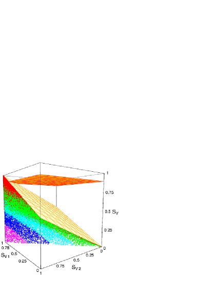
(a)

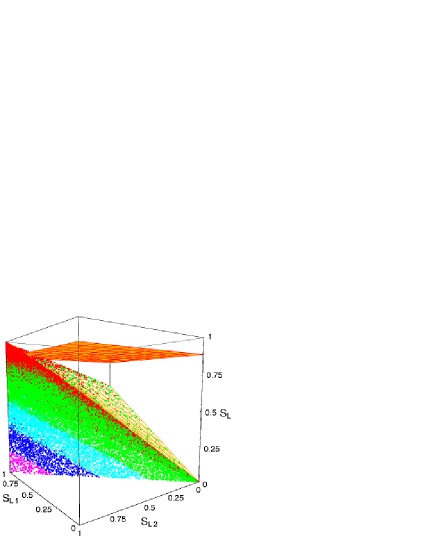
(b)

Figure 1: Plots of 60,000 randomly generated physical states of two qubits in the space of global and marginal mixednesses, as quantified by Von Neumann entropy (a), or linear entropy (b). Red dots indicate separable states; green, cyan, blue, and magenta dots denote nonseparable states. The entanglement of formation (a), or tangle (b), grows going from the green to the magenta zone (see text for details). In both plots, the yellow surfaces represent product states, while above the red-orange planes no entangled states can be found. All quantities plotted are dimensionless.

IV Characterizing Entanglement in the Space of Linear Entropies

We now consider the linear entropy as a measure of mixedness. The advantage of using the linear entropy is that it is directly related to the purity of the state by Eq. (2), and its definition does not involve any transcendental function. In this case the entanglement is properly quantified by the tangle $\tau(\rho)\equiv\mathcal{C}^{2}(\rho)$ because the linear entropy of entanglement for pure states is related to the Von Neumann entropy of entanglement Eq. (3) by the same relationship that connects the tangle to the entanglement of formation. We again randomly generate some thousands density matrices $\rho$ of two qubits and plot them as points in the three-dimensional space ${\mathcal{E}}_{L}\equiv\left\{S_{L1}\equiv S_{L}(\rho_{1}),\,S_{L2}\equiv S_{L}(\rho_{2}),\,S_{L}\equiv S_{L}(\rho)\right\}$, as shown in Fig. 1(b). The distribution of colored bundles is analogous to that of the previous case Fig. 1(a), but with the linear entropies and the tangle replacing, respectively, the Von Neumann entropies and the entanglement of formation.

A comparison with the previous case shows some prima facie analogies and some remarkable differences. We find again a general trend of increasing entanglement with decreasing global and increasing marginal mixednesses. Product states lie on the yellow surface of equation $S_{L}=2(S_{L1}+S_{L2})/3-(S_{L1}S_{L2})/3$. With respect to the linear entropy, taken as a measure of mixedness, they are not maximally mixed states with fixed marginals. This fact has deep consequences that we will explore in Sec. VI. Going downward through Fig. 1(b) we find a small region of only separable states above the horizontal red-orange plane $S_{L}=8/9$ Nemoto . Below this plane there is again the region of coexistence of separable and entangled states, while in the region of lowest global and largest marginal mixednesses we find only entangled states. Pure states are always located at $S_{L}=0$ on the line $S_{L1}=S_{L2}$, and again, there are no states for $S_{L}=0$ and $S_{L1}\neq S_{L2}$. Qualitatively, the structure is very similar to that obtained in the space ${\mathcal{E}}_{V}$ of Von Neumann entropies. Some numerics changes due to different definitions, in particular the lower boundary of the region of coexistence is now determined by the entropic criterion for the linear entropies: if a state is separable, then $S_{L}\geq 2(\max\{S_{L1},\,S_{L2}\})/3$, or, equivalently, $\mu\leq\min\{\mu_{1},\,\mu_{2}\}$. A state violating these inequalities must necessarily be entangled. The tangle satisfies a numerical upper bound analogous to Eq. (9) for the entanglement of formation,

$$\mathcal{C}^{2}(\rho)\leq\min\{S_{L1},\,S_{L2}\}\;.$$ (12)

V MEMMS in the Space of Linear Entropies: Analytical Bounds

Obviously, states of the form Eq. (11) are MEMMS in the space ${\mathcal{E}}_{L}$ as well. The relation between the eigenvalues $x_{i}$ of the reduced density matrices $\rho_{m_{i}}$ and the tangle is $\mathcal{C}^{2}(\rho_{m})=4x_{1}x_{2}$, while for the marginal linear entropies we have $S_{Li}=2[x_{i}^{2}+(1-x_{i})^{2}]$. This time we can straightforwardly invert these relations to obtain the following analytical upper bound on the tangle of any mixed state of two qubits (see Fig. 2)

$$\mathcal{C}^{2}(\rho)\leq\left(1\mp\sqrt{1-S_{L1}}\right)\left(1\pm\sqrt{1-S_{L2}}\right)\,,$$ (13)

where the minus sign must be associated with the lowest marginal linear entropy. For equal marginals this bound reduces simply to $\mathcal{C}^{2}(\rho)\leq S_{L1}=S_{L2}$ and the equality is reached for pure states. The bound Eq. (13) bears some remarkable consequences. In particular, it entails that maximal entanglement decreases at a very fast rate with increasing difference of marginal linear entropies, as can be seen in Fig. 2. In fact, it introduces the following general rule: in order to obtain maximally entangled states one needs to have the lowest possible global mixedness, the largest possible marginal mixednesses, and the smallest possible difference between the latter. That the marginals should be as close as possible is intuitively clear, because if the two subsystems have strong quantum correlations between them, they must carry about the same amount of information. For instance, the MEMS defined in Ref. Munro have always the same marginal spectra. The marginals should be large as well: in particular, if the mixedness of one of the subsystems is zero, then the state of the total system is not entangled. Finally, from Eqs. (5) and (13) it immediately follows that the entanglement of formation satisfies the following bound:

$$E_{F}(\rho)\leq{\mathcal{F}}\left(\sqrt{\left(1\mp\sqrt{1-S_{L1}}\right)\left(1\pm\sqrt{1-S_{L2}}\right)}\right)\,.$$ (14)

This bound establishes a relation between the entanglement of a mixed state and its marginal mixednesses. Although the entanglement of formation for systems of two qubits is known Wootters , our inequality Eq. (14) provides a generalization to mixed states of the equality $E_{F}(\rho_{p})=\mathcal{F}\left(\sqrt{S_{L}(\rho_{p_{1,2}})}\right)$ holding for pure states.

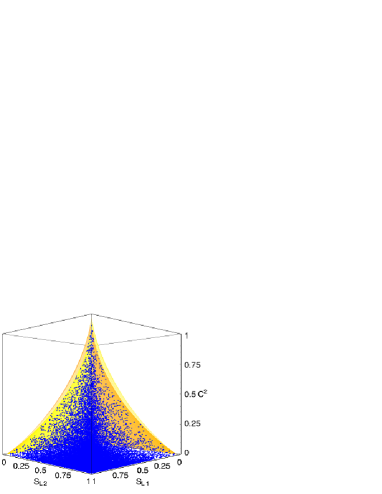
Figure 2: Plot of the tangle $\mathcal{C}^{2}(\rho)$ as a function of the marginal linear entropies for 30,000 randomly generated entangled states of two qubits. The yellow shaded surface represents the maximally entangled states for fixed marginal mixednesses (MEMMS) defined by Eq. (11). They saturate the inequality Eq. (13). All quantities plotted are dimensionless.

VI LPTPS: Entangled States that are Less Pure than Product States

Unlike the Von Neumann entropy, the linear entropy is not additive on product states, and does not satisfy the triangle inequality. As mentioned above, with respect to the linear entropy, product states are not maximally mixed states with fixed marginal mixednesses (see Fig. 1(b)), and this entails the existence of states (separable or entangled) that are less pure than product states (LPTPS). We wish to characterize the entangled LPTPS and to study their tangle as a function of their “distance in purity” from product states. Because for the latter $\mu=\mu_{1}\mu_{2}$, then for any state $\rho$ to be a LPTP state (separable or entangled) the following condition must hold:

$$\Delta\mu\equiv\mu_{1}\mu_{2}-\mu\geq 0\;,$$ (15)

where $\Delta\mu$ defines the natural distance from the purity of product states. The LPTPS that saturate inequality Eq. (15) are isospectral to product states. We are looking for entangled LPTPS, and we can then exploit again the form Eq. (10) of the density matrix, and impose the condition Eq. (15) to obtain the following constraints:

$$\left\{\begin{array}[]{ll}1-2x_{1}-2x_{2}+2x_{1}x_{2}\geq 0\\ c^{2}\leq 4x_{1}x_{2}(1-2x_{1}-2x_{2}+2x_{1}x_{2})\;.\end{array}\right.$$ (16)

For all entangled LPTPS this implies that

$$S_{L1,2}\leq\frac{4\sqrt{1-S_{L2,1}}}{\left(1+\sqrt{1-S_{L2,1}}\right)^{2}}\;,$$ (17)

which simply means that no entangled states can exist too close to the maximally mixed state, as shown in Fig. 3(a). In the range of parameters $\{c,x_{1},x_{2}\}$ constrained by Eq. (16), it is immediately verified that the largest eigenvalue of the density matrix Eq. (10) is always smaller than the largest eigenvalues of the marginals $\rho_{1,2}$ so that entangled LPTPS are never detected by the majorization criterion. We now wish to determine the maximally entangled LPTPS with fixed $\Delta\mu$. This problem can be easily recast as a constrained maximization of $\Delta\mu=x_{1}x_{2}(1-2x_{1}-2x_{2}+2x_{1}x_{2})/2-c^{2}$ with fixed $c$. Its solution yields a class of states with $x_{1}=x_{2}=(3-\sqrt{5})/4$, and a linear relation between the distance $\Delta\mu$ and the tangle $c^{2}$:

$$c^{2}=2(\Delta\mu_{\max}-\Delta\mu)\;,$$ (18)

where $\Delta\mu_{\max}=(5\sqrt{5}-11)/8\simeq 0.0225$. The tangle of maximally entangled LPTPS decreases linearly with increasing $\Delta\mu$ from the maximum value $c^{2}_{\max}=2\Delta\mu_{\max}$ at $\Delta\mu=0$, and vanishes beyond the critical value $\Delta\mu_{\max}$ (See Fig. 3(b)). When the mixednesses are measured using the Von Neumann entropy, one finds that all LPTPS lie below the plane of product states in the space ${\mathcal{E}}_{V}$ (See Fig. 1(a)). Therefore, in this case, the lack of precision with which the linear entropy characterizes the Von Neumann entropy turns out to be an useful resource to detect a class of entangled states that could not be otherwise discriminated by the entropic and majorization criteria.

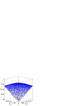
(a)

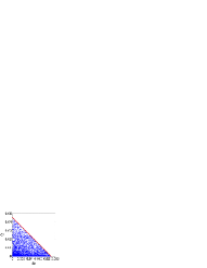
(b)

Figure 3: Entangled LPTPS. (a) Plot of 10,000 numerically generated entangled LPTPS in the space ${\mathcal{E}}_{L}$ of global and marginal linear entropies. As in Fig. 1(b), the yellow surface represents product states. (b) Plot of the tangle $\mathcal{C}^{2}(\rho)$ of LPTPS as a function of the distance $\Delta\mu$ from the purity of product states. The red line represents the maximally entangled LPTPS given by Eq. (18). All quantities plotted are dimensionless.

VII Concluding Remarks and Outlook

In conclusion, we explored and characterized qualitatively and quantitatively the entanglement of physical states of two qubits by comparing their global and marginal mixednesses, as measured either by the Von Neumann or the linear entropy. We found that entanglement generally increases with decreasing global mixedness and with increasing local mixednesses, and we provided several numerical bounds. We determined the class of maximally entangled states with fixed marginal mixednesses (MEMMS). They allow to obtain an analytical upper bound for the entanglement of formation of generic mixed states in terms of the marginals. This provides a partial generalization to mixed states of the exact equalities holding for pure states. We may reasonably expect that similar bounds and inequalities can be determined for more complex systems that do not allow for a direct computation of entanglement measures.

The difference between linear and Von Neumann entropies allows to detect a class of states that are less pure than product states with fixed marginal mixednesses (LPTPS). We characterized the entangled LPTPS and showed that their maximal entanglement decreases with decreasing purity. Finally, we singled out in both spaces ${\mathcal{E}}_{V}$ and ${\mathcal{E}}_{L}$ a large region of coexistence of separable and entangled states with the same global and marginal mixednesses. In this region a complete characterization of entanglement can be achieved only once the amount of classical correlations in a quantum state has been properly quantified. This problem awaits further study, as well as the question of characterizing entanglement with global and marginal mixednesses for higher–dimensional and continuous variable systems.

- (1) M. A. Nielsen and I. L. Chuang, Quantum Computation and Quantum Information (Cambridge University Press, Cambridge, 2000); Fundamentals of Quantum Information, D. Heiss Ed. (Springer–Verlag, Berlin, 2002).
- (2) B. Schumacher, Phys. Rev. A 54, 2614 (1996).
- (3) S. Lloyd, Science 261, 1589 (1993); D. P. DiVincenzo, ibid. 270, 255 (1995).
- (4) A. K. Ekert, Phys. Rev. Lett. 67, 661 (1991).
- (5) C. H. Bennett, G. Brassard, C. Crépeau, R. Jozsa, A. Peres, and W. K. Wootters, Phys. Rev. Lett. 70, 1895 (1993).
- (6) K. Życzkowski, P. Horodecki, A. Sanpera, and M. Lewenstein, Phys. Rev. A 58, 883 (1998).
- (7) S. Ishizaka and T. Hiroshima, Phys. Rev. A 62, 022310 (2000); F. Verstraete, K. Audenaert, and B. De Moor, Phys. Rev. A 64, 012316 (2001).
- (8) W. J. Munro, D. F. V. James, A. G. White, and P. G. Kwiat, Phys. Rev. A 64, 030302 (2001).
- (9) T.-C. Wei, K. Nemoto, P. M. Goldbart, P. G. Kwiat, W. J. Munro, and F. Verstraete, Phys. Rev. A 67, 022110 (2003).
- (10) R. F. Werner, Phys. Rev. A, 40, 4277 (1989).
- (11) Regarding the entropy of entanglement of pure states in two–qubit systems, the Von Neumann and the linear entropy are equivalent because , where the convex monotonic function is defined by Eq. (6).
- (12) M. A. Nielsen and J. Kempe, Phys. Rev. Lett. 86, 5184 (2001).
- (13) R. Horodecki, P. Horodecki, and M. Horodecki, Phys. Lett. A 210, 377 (1996); R. Rossignoli and N. Canosa, Phys. Rev. A 66, 042306 (2002).
- (14) A. Peres, Phys. Rev. Lett. 77, 1413 (1996); M. Horodecki, P. Horodecki, and R. Horodecki, Phys. Lett. A 223, 1 (1996).
- (15) C. H. Bennett, D. P. DiVincenzo, J. A. Smolin, and W. K. Wootters, Phys. Rev. A 54, 3824 (1996).
- (16) W. K. Wootters, Phys. Rev. Lett. 80, 2245 (1998).
- (17) We generate the eigenvalues of each density matrix randomizing in under the constraint . Then we rotate the matrix back in the computational basis with a random unitary transformation.
- (18) H. Araki and E. H. Lieb, Comm. Math. Phys. 18 160 (1970); A. Wehrl, Rev. Mod. Phys. 50, 221 (1978).