Dipolar Relaxation in an ultra-cold Gas of magnetically trapped chromium atoms

Abstract

We have investigated both theoretically and experimentally dipolar relaxation in a gas of magnetically trapped chromium atoms. We have found that the large magnetic moment of 6 $\mu_{B}$ results in an event rate coefficient for dipolar relaxation processes of up to $3.2\cdot 10^{-11}$ cm³s^-1 at a magnetic field of 44 G. We present a theoretical model based on pure dipolar coupling, which predicts dipolar relaxation rates in agreement with our experimental observations. This very general approach can be applied to a large variety of dipolar gases.

1 Introduction

Recently, the dipole-dipole interaction in Bose-Einstein condensates has generated significant theoretical interest Baranov2002 . It has been shown that the long-range character and the anisotropic nature of the interaction between magnetic or electric dipoles will lead to many interesting new phenomena like novel quantum phase transitions Goral2002 , dipolar order Pu2001 and spin tunnelling Pu2002 in the condensate. New questions concerning stability Goral2000 ; Yi2001 and tunability of the interaction Giovanazzi2002 of such a condensate arise. In most of the recent work, the interaction between dipoles is treated as completely elastic. However, in a typical experiment aimed at the creation of a Bose-Einstein condensate, the atoms are held in a magnetic trap in the energetically highest magnetic sub-level. Therefore, inelastic dipolar relaxation processes in which the atomic spin flips and the Zeeman energy is released cannot a priori be neglected.

Most of the above proposals require a large dipole moment like the one of a polar molecule in an electric field. In this paper, we show theoretically and experimentally that already for chromium with a magnetic moment of 6 $\mu_{B}$ heating and atom loss due to dipolar relaxation is so significant that it is impossible to reach Bose-Einstein condensation by the standard procedure of rf-evaporation in a magnetic trap.

Using a simple model which only takes into account the dipolar interaction and neglects all other aspects of the molecular interaction on the scattering process we are able to explain the observed dipolar relaxation rate in ultra-cold ⁵²Cr. Qualitatively, we find the same behavior for ⁵⁰Cr. This gives strong evidence that, in the absence of resonant behavior, inelastic collisions due to dipolar relaxation can be treated in a very general way.

2 Dipolar Relaxation: Theory

As a consequence of Maxwell’s equations it is impossible to create a maximum of a static magnetic field in a region where external currents are absent. For this reason atoms are usually magnetically trapped in the energetically highest Zeeman sub-level (weak-field-seeking state). The trap lifetime of these atoms is mainly limited by collisions. Aside from background gas collisions and three-body recombination, the atoms undergo spin-exchange and dipolar relaxation collisions. In contrast to spin-exchange collisions, where the total spin is conserved, the spin is flipped in a dipolar relaxation process since dipole-dipole interaction does not preserve the total spin, but rather the total angular momenta. Therefore, if one considers a cloud of fully polarized atoms in the energetically highest state, only spin relaxation which does not conserve the total spin leads to atom loss from the magnetic trap.

Here, we estimate the inelastic cross sections for spin-flip transitions due to the magnetic spin-dipole spin-dipole interaction using Fermi’s Golden rule. A similar form of this approximation, equivalent to the Born approximation, has already been considered in Shlyapnikov1994 ; Fedichev1996 , for calculating the dipolar relaxation rates of meta-stable triplet helium. In particular, in Fedichev1996 it is shown that the bare Born approximation is reasonably consistent with the distorted-wave approximation which is a true first order calculation. Because of the small dipole-dipole coupling in polarized triplet helium ($S=1$), the latter is considered to be an almost exact approach.

For chromium, the situation is slightly different because the magnetic coupling is larger. A first order calculation, in the form of the Born approximation, provides us with an approximate analytical tool for the interpretation of the experimental results, but may not be expected to be as accurate as in the case of metastable helium.

We consider for simplicity the case of two identical atoms trapped in the energetically highest sub-level of the Zeeman manifold. Moreover, we consider the case of zero electronic angular momenta $L=0$ such that the magnetic interaction solely arises from the electronic spin. The long range part of the interaction between two atomic magnetic dipole moments $\vec{\mu}_{1}=g_{S}\mu_{B}\vec{S}_{1}$ and $\vec{\mu}_{2}=g_{S}\mu_{B}\vec{S}_{2}$ located at ${\bf r}_{1}$ and ${\bf r}_{2}$, where $\vec{S}_{1}$ and $\vec{S}_{2}$ are the two spin matrices, reads

$$U_{\mathrm{dd}}(\vec{r})=\mu_{0}(g_{S}\mu_{B})^{2}\,{(\vec{S}_{1}\cdot\vec{S}_{2})-3\,(\vec{S}_{1}\cdot\hat{\vec{r}})\,(\vec{S}_{2}\cdot\hat{{\bf r}})\over 4\pi r^{3}}.$$ (1)

Here we have introduced the interatomic separation $\vec{r}=\vec{r}_{2}-\vec{r}_{1}$ with $\hat{\vec{r}}=\vec{r}/r$ and the magnetic permeability of the vacuum $\mu_{0}$. The tensorial part of the dipolar interaction (1), namely $(\vec{S}_{1}\cdot\vec{S}_{2})-3\,(\vec{S}_{1}\cdot\hat{\vec{r}})\,(\vec{S}_{2}\cdot\hat{\vec{r}})$ can be rewritten in terms of spin-flip operators:

$$S_{1z}\cdot S_{2z}+{1\over 2}\left(S_{1+}\cdot S_{2-}+S_{1-}\cdot S_{2+}\right)$$

$$-{3\over 4}\left(2\;\hat{z}S_{1z}+\hat{r}_{-}S_{1+}+\hat{r}_{+}S_{1-}\right)$$ (2)

$$\times\left(2\;\hat{z}S_{2z}+\hat{r}_{-}S_{2+}+\hat{r}_{+}S_{2-}\right)$$

where

$$\hat{z}={z\over r},\;\;\;\;\;\hat{r}_{+}={x+iy\over r},\;\;\;\;\;\hat{r}_{-}={x-iy\over r},$$ (3)

and where $S_{+}=(S_{x}+iS_{y})/\sqrt{2}$ and $S_{-}=(S_{x}-iS_{y})/\sqrt{2}$ are ladder operators of the spin operators. From the above expression (2) it can be seen that in first order Born approximation each single atom can flip at most one spin ($\Delta m_{S}=1$) and in total for the two-atoms system $\Delta m_{S}=2$.

In the Born approximation the total cross section for two identical colliding atoms in the same internal state can be expressed in the following form

$$\sigma=\left(\frac{m}{4\pi\hbar^{2}}\right)^{2}{1\over kk_{f}}\left[\int|\tilde{U}_{\mathrm{dd}}(\vec{k}-\vec{k}^{\prime})|^{2}\delta(|\vec{k}^{\prime}|-k_{f})\,d\vec{k}^{\prime}\right.$$

$$\left.\pm\int\tilde{U}_{\mathrm{dd}}(\vec{k}-\vec{k}^{\prime})\tilde{U}_{\mathrm{dd}}^{*}(-\vec{k}-\vec{k}^{\prime})\delta(|\vec{k}^{\prime}|-k_{f})\,d\vec{k}^{\prime}\right]\,$$ (4)

where $\vec{k}$ and $\vec{k}^{\prime}$ are the initial and final wave vectors, respectively, $k_{f}$ is the modulus of the final state wave vector. $\tilde{U}_{\mathrm{dd}}(\vec{q})$ is the Fourier transform of the dipole-dipole interaction (1) already contracted between the (symmetric) spin (or internal state) functions of initial and final states. The sign $\pm$ of the second term in the square bracket, the ”exchange” term, depends on particle’s symmetry: $+$ holds for bosons and $-$ for fermions. When the two colliding atoms are not in the same internal state a generalization of (4) with both signs should be used.

2.1 Dipolar transitions in a dipolar Bose gas

We have in mind the specific case of ⁵²Cr atoms in the electronic ground state, magnetically trapped in the highest Zeeman sub-level. For ⁵²Cr, both the nuclear spin and the electron orbital momentum vanish (I=0, L=0), and only the electron spin is finite ($S=3$). The degeneracy of the 2S+1 atomic ground state sub-levels is lifted by a magnetic field $B$. The Zeeman splitting is given by

$$\Delta E=g_{S}\mu_{B}B$$ (5)

where $\mu_{B}$ is the Bohr magneton and $g_{S}$ is the Land$\acute{e}$ factor ($g_{S}=2$). The magnetic field is chosen along the $z$ direction and determines the quantization axis. We label the internal states via the $z$-component of the total internal angular momentum (in this specific case only the electronic spin), like $|m_{S}\rangle$.

We consider specifically the case in which both atoms are prepared in the stretched state, i.e $|m_{S}=s\rangle$. The total spin function of the two colliding particles is already symmetric and will be denoted as $|s;s\rangle$. The possible final internal states of the two colliding atoms are

$$|f_{0}\rangle = |s;s\rangle$$ (6)

$$|f_{1}\rangle = {\left(|s;s-1\rangle+|s-1;s\rangle\right)\over\sqrt{2}}$$ (7)

$$|f_{2}\rangle = |s-1;s-1\rangle$$ (8)

where the subscripts $0,1,2$ refer to the number of spins that are flipped. For dipolar scattering, the total cross section will depend on the relative orientation of the initial relative momentum ${\bf k}$ and the polarization axes. The averaged cross sections over all possible orientations for the $0$, $1$ and $2$ spin-flip processes reads

$$\sigma_{0} = {16\pi\over 45}S^{4}\left(\frac{\mu_{0}(g_{S}\mu_{B})^{2}m}{4\pi\hbar^{2}}\right)^{2}\left[1+h(1)\right]$$ (9)

$$\sigma_{1} = {8\pi\over 15}S^{3}\left(\frac{\mu_{0}(g_{S}\mu_{B})^{2}m}{4\pi\hbar^{2}}\right)^{2}\left[1+h(k_{f}/k_{i})\right]{k_{f}\over k_{i}}$$ (10)

$$\sigma_{2} = {8\pi\over 15}S^{2}\left(\frac{\mu_{0}(g_{S}\mu_{B})^{2}m}{4\pi\hbar^{2}}\right)^{2}\left[1+h(k_{f}/k_{i})\right]{k_{f}\over k_{i}}.$$ (11)

While $\sigma_{1}$ and $\sigma_{2}$ are the cross sections for dipolar relaxation, $\sigma_{0}$ is the contribution to the elastic cross section due to the dipole-dipole interaction. Here

$$h(x)=-{1\over 2}-{3\over 8}{(1-x^{2})^{2}\over x(1+x^{2})}\log\left({(1-x)^{2}\over(1+x)^{2}}\right)$$ (12)

represents the ratio of the exchange contribution to the direct one of Eq. (4). The function $h$ (see Fig 1) is defined in the interval (1,$\infty$) and exhibits a monotonic increase from h(1)=-1/2 to $h(\infty)=1$. (For large values of the argument $h(x)\approx 1-4/x^{2}$.)

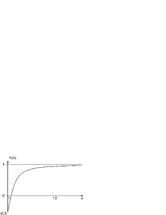
Figure 1: Function h(x); h(x) is a monotonically increasing function which asymptotically approaches 1.

Note, that the term in brackets in Eq. (11) can be expressed in terms of the classical electron radius $r_{0}$, atomic mass $m$ and electronic mass $m_{e}$:

$$\left(\frac{\mu_{0}(g_{S}\mu_{B})^{2}m}{4\pi\hbar^{2}}\right)^{2}=\left(\frac{m}{m_{e}}\right)^{2}r_{0}^{2}\,.$$ (13)

One can see that the explicit dependence on $\hbar$ disappears.

The factor ${k_{f}\over k_{i}}$ accounts for the different density of final states in the inelastic process ($\Delta E\neq 0$). The ratio between final and initial wave-vectors is $k_{f}/k_{i}=\sqrt{1+{m\Delta E\over\hbar^{2}k_{i}^{2}}}$ for a one spin-flip transition and $k_{f}/k_{i}=\sqrt{1+{2m\Delta E\over\hbar^{2}k_{i}^{2}}}$ for a two spin-flip transition. If the Zeeman energy is larger than the initial kinetic energy it exhibits a characteristic $\sqrt{B}$ dependence. The expressions in Eq. (11) for one and two spin flip processes can also be applied to meta-stable helium ($S=1$). For $B=0$ we recover the result of Shlyapnikov1994 ; Fedichev1996 for one and two spin-flip process (using $\langle v_{rel}\rangle=\sqrt{16k_{B}T/\pi m}$ ). Our method yields an analytical solution for all values of the magnetic field which reproduces the magnetic-field dependence found in Shlyapnikov1994 ; Fedichev1996 at very small and large magnetic field.

3 Experiments

3.1 Dipolar relaxation in chromium

The magnetically trappable substates in the ${}^{7}S_{3}$ ground state of chromium are the low-field seeking states $m_{S}=1,2,3$. In a polarized sample of atoms in the energetically highest state ($m_{S}=3$), there are two possible decay channels due to dipolar relaxation:

$$|3;3\rangle,|3;3\rangle \rightarrow |3;3\rangle,|3;2\rangle+\Delta E$$

$$|3;3\rangle,|3;3\rangle \rightarrow |3;2\rangle,|3;2\rangle+2\Delta E.$$ (14)

In these processes either one or both colliding atoms change their state to the $m_{S}=2$ state and release a Zeeman-energy of $\Delta E$ or $2\Delta E$, respectively. The energy is equally distributed among the colliding atoms. In a single spin flip transition the increase in temperature which corresponds to the released Zeeman energy $\left(3k_{B}\Delta T\right.=\left.\Delta E/2\right)$ is 250$\,\mu$K for an offset field of$B_{0}$=$10$ G. This is generally not high enough to eject the atoms from the trap. As a consequence thermalization leads to heating of the trapped cloud (see Fig. 2(a)). The increasing population of the $m_{S}=2$ state opens additional collision channels due to spin exchange collisions and dipolar relaxation between identical and different states. The sample becomes more and more depolarized and only collisions with a final state of $m_{S}<1$ lead to atom loss. In this paper, we concentrate on dipolar relaxation of $m_{S}=3$ state atoms in an almost spin-polarized sample.

3.2 Methods to determine the dipolar relaxation rate

In the following, we present three experimental methods from which we obtain the dipolar relaxation coefficient $\beta_{dr}$ for the $m_{S}=3$ state. It can be determined by measuring either the decreasing population (method (i), (ii)) of this state or the heating of the atom cloud in the trap (method (iii)) over time. Methods (i) and (iii) have also been used in Guery-Odelin1998 to determine the dipolar relaxation rate of Cs in the F=3 ground state.

The atom loss from the $m_{S}=3$ state of an initially polarized sample of $N_{3}$ atoms is described by

$$\frac{dN_{3}(t)}{dt}=-\int{\Gamma(\vec{r},t)n_{3}(\vec{r},t)\>d^{3}r},$$ (15)

where $n_{3}(\vec{r},t)$ and $\Gamma(\vec{r},t)$ are the position and time-dependent atom density and loss rate, respectively. $\Gamma(\vec{r},t)$ can be written as

$$\Gamma(\vec{r},t)=\gamma_{bg}+\beta_{dr}n_{3}(\vec{r},t)+\widetilde{\Gamma}(\vec{r},t).$$ (16)

Here background gas collisions with a rate coefficient $\gamma_{bg}$ are represented by the first term and the density-dependent dipolar relaxation with a rate constant $\beta_{dr}$ by the second term. Other collisional losses e.g. three-body recombination, relaxation and spin-exchange processes which involve states other than the $m_{S}=3$ state are included in $\widetilde{\Gamma}(\vec{r},t)$. For low densities and small populations in these other states, this term can be neglected.

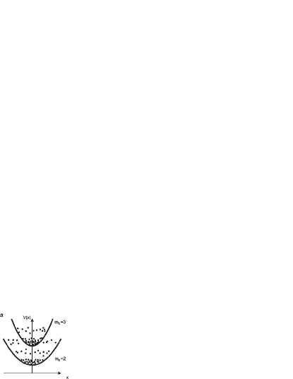
Figure 2: a) Dipolar relaxation in a magnetic trap. Atoms initially prepared in the $m_{S}=3$ state undergo dipolar relaxation and fill the $m_{S}=2$ state. Indicated is the energy gain of a colliding atom of $\Delta$E/2 and $\Delta$E of single and double spin flip transition, respectively. Thermalization of the released Zeeman energy leads to heating in the trap. b) If a rf-shield is applied, the collisional products leave the trap. Thus, the collision process is turned into a real loss process.

The first method (i) takes advantage of the Zeeman-energy gain during a relaxation process. The energetic collisional products are selectively removed by a radio-frequency (rf) shield with frequency $\nu_{\mathit{rf}}$ as depicted in Fig. 2. Thus, dipolar relaxation is turned into a real loss process and can directly be measured by monitoring the remaining atoms. The decay is fitted to the solution of the differential equation:

$$\frac{dN_{3}(t)}{dt}=-\gamma_{bg}N_{3}(t)-{\beta}^{\circ}_{dr}\frac{N_{3}^{2}(t)}{\overline{V}(t)}.$$ (17)

Where $\overline{V}=\sqrt{8}(2\pi)^{3/2}\sigma_{x}\sigma_{y}\sigma_{z}$ is the mean volume of an atomic cloud with a Gaussian density distribution with 1/$\sqrt{e}$ widths $\sigma_{x,y,z}$. To remove the collisional products the rf-frequency of the shield has to be chosen such that $m_{J}(h\nu_{\mathit{rf}}-\Delta E)<\Delta E/2$. In this case $\beta^{\circ}_{dr}$ is an event rate which contains single and double spin flip transitions. $\beta^{\circ}_{dr}$ can be calculated from the thermal average over both inelastic collision channels:

$$\beta^{\circ}_{dr}=2\cdot\langle(\sigma_{1}+\sigma_{2})v_{rel}\rangle_{{}_{therm}}.$$ (18)

The factor of $2$ accounts for two removed atoms per collision event. At the same time, the rf-frequency has to be adjusted to a sufficiently high value, such that the initial $m_{S}=3$ cloud is not significantly evaporated ($h\nu_{\mathit{rf}}\gg\Delta E+k_{B}T$, where T is the initial temperature of the cloud). From the above considerations it becomes clear that for a given temperature this method is only applicable for offset fields $B_{0}\gg 3k_{B}T/\mu_{B}$.

For smaller magnetic offset fields, we use a second method (ii). The initially polarized cloud evolves in the magnetic trap for a certain time $t$. By applying a strong magnetic field gradient after switching off the trap, the magnetically trapped atoms can be spatially separated with respect to their substates before imaging. This is equivalent to a Stern-Gerlach experiment. A series of these images yields the time evolution of the population of the trappable sub-levels. From the initial decay of the $m_{S}=3$ we obtain the loss rate $\widetilde{\beta}_{dr}$.

$$\frac{dN_{3}(t)}{dt}=-\gamma_{bg}N_{3}(t)-\widetilde{\beta}_{dr}\frac{N_{3}^{2}(t)}{\overline{V}(t)}.$$ (19)

It is not possible to distinguish between single (one atom lost from $m_{S}=3$)and double (two atoms lost from $m_{S}=3$) spin flip transitions with this method. Hence the relation between $\widetilde{\beta}_{dr}$ and the cross sections changes to

$$\widetilde{\beta}_{dr}=\langle(\sigma_{1}+2\cdot\sigma_{2})v_{rel}\rangle_{{}_{therm}}.$$ (20)

The practicability of this method is limited by the magnitude of the magnetic field gradient which can be applied to separate the expanding thermal clouds before imaging.

The third method (iii) measures the heating of the atomic cloud due to the energy released by dipolar relaxation processes. The evolution of the temperature is given by

$$\frac{dT(t)}{dt}=\widetilde{\beta}_{dr}\frac{N_{3}(t)}{\overline{V}(t)}\Delta T.$$ (21)

Since a two spin flip transition yields twice the energy of a single spin flip transition the obtained value is $\widetilde{\beta}_{dr}$ as in method (ii) (Eq.20). This method requires that the cloud is in thermal equilibrium, i.e. that rethermalization by elastic collisions is faster than the dipolar relaxation process itself. As the velocity of atoms which have undergone a dipolar relaxation event and the volume which is occupied by the collisional products increases with increasing offset field, the elastic collision rate drops and impairs the measured result.

3.3 Preparation of the sample and experimental methods

The basic setup used in our experiments has been described previously Schmidt20031 ; Schmidt20033 and is only briefly summarized in the following. Zeeman-slowed ⁵²Cr atoms are magneto-optically trapped in the magnetic field configuration of a Ioffe–Pritchard trap in the cloverleaf configuration using the ⁷S₃-⁷P₄ transition. Since this transition is not closed, we populate the metastable ⁵D₄ state via the weak ⁷P₄-⁵D₄ intercombination line. In this state the atoms are decoupled from the trapping light and can be magnetically trapped because of the high magnetic moment ($6\mu_{B}$). We load about $2\cdot 10^{8}$ atoms continuously in the Ioffe–Pritchard type trap (”CLIP”–trap Schmidt20032 ). After switching off the trapping light, we optically transfer (using light at 658 nm) the atoms back to the ⁷S₃ ground state, which possesses the same magnetic moment($\mu=6\mu_{B}$). Subsequently, we compress the sample and perform Doppler cooling in the magnetic trap. Using this method, we obtain a nearly polarized ($m_{S}=3$) atomic ensemble with an initial density of about $10^{11}$ atoms/cm³ and a temperature of $275\pm 25\,\mu$K.

This is the starting point for most of our measurements of dipolar relaxation at high magnetic offset fields ($17-44$ G) using method (i). However, for smaller offset fields ($<$25 G), it was necessary to reduce the temperature further by rf-evaporation to realize a cut-off parameter for the rf-shield of $\eta\geq 5$ Masuhara1988 . After preparation, the rf-shield is applied and the atomic ensemble is allowed to evolve in the trap for a variable time $t$. The rf-frequency is set to $1$ MHz below $7\Delta E/6h$. Subsequently, the shadow of the atoms is imaged onto a CCD-camera by illuminating the atoms for $100\,\mu$s with a circularly polarized beam after $5$ ms of free ballistic expansion in a homogenous magnetic field.

The number of remaining atoms $N_{3}(t)$ and the mean volume $\overline{V}(t)$ are extracted from a 2D-Gauss fit to absorption images using the separately measured trap frequencies (at $27$ G offset field: $\nu_{radial}=120$ Hz, $\nu_{axial}=73$ Hz). A series of these measurements with different evolution times $t$ yields $N_{3}(t)$. The temperature $T(t)$ is obtained by recording the ballistic expansion of the atom cloud at different evolution times.

For measurements at low offset fields ($<$2 G), we use the second approach (ii). Since the temperature obtained after Doppler cooling is too high to separate the atoms with the available field gradient, we reduce the temperature of the sample to $50\,\mu$K by rf-evaporative cooling at an offset field of 0.7 G (trap frequencies for this configuration are typically $\nu_{radial}=806$ Hz, $\nu_{axial}=42$ Hz). Subsequently, we turn off the rf-frequency and change the offset field for a free evolution time $t$ to the desired value. Shortly (10 ms) before the Stern-Gerlach sequence, the field is changed back to 0.7 G.

The separation of the substates is accomplished by switching off the axially confining pinch and bias fields of our clover-leaf trap and simultaneously applying a homogenous field in the imaging direction which is perpendicular to the offset field direction and diagonal to the leaf position of our trap. By this means the center of the trap is displaced radially and the atoms get accelerated in the gradient field of the leaves ($170$ G/cm) along an axis perpendicular to the imaging direction. After a $1.7$ ms acceleration phase, all magnetic fields are turned off and the atoms expand freely for another $5$ ms before the spatially separated clouds are imaged on the CCD camera by illuminating them for $1$ ms with a calibrated light field. The data analysis is perform by averaging three pictures taken under identical experimental conditions for each evolution time. An example for such an image taken at $0.3$ G is depicted in Fig. 3.

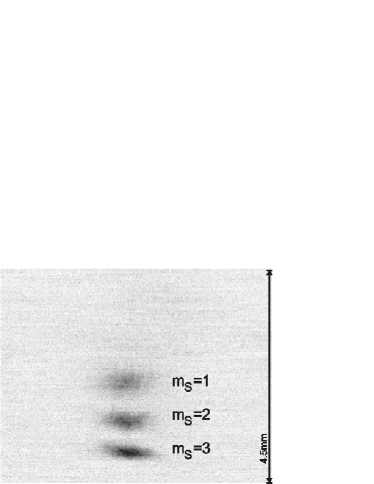
Figure 3: Typical fluorescence picture taken after separation of the sub-levels in a Stern-Gerlach type experiment and $5$ ms time of flight. The sub-levels have been accelerated downwards.

The clouds have been accelerated downwards. The cloud containing atoms in the energetically highest state ($m_{S}=3$) therefore appears at the lowest position.

The number of atoms in each substate are obtained by 2D-Gauss fits within an equally sized rectangular area around each cloud. Because of the long exposure time and the trap geometry being changed while switching off the trap, temperature and volume were obtained in separate measurements where we record the free expansion of the whole cloud at different evolution times with a exposure time of $200\,\mu$s.

We determine the offset field by probing the minimum of the trapping field via rf removal of trapped atoms. The achieved accuracy of the values is about 300 mG for measurements at high offset values and 100 mG for the measurements at low offset fields. The background gas collision rate $\gamma_{bg}=1/200$ s is obtained from a separate measurement with a low density atomic sample. This reduces the fitting parameters to the initial number of atoms and $\beta_{dr}$. The increasing volume due to heating during the measurement was included in the fit. The errors in the determination of the number of atoms is about 30%. The error bars shown in the figures are the square root of the diagonal elements of the covariance matrix for the fitting parameters obtained from a least-squares fit.

3.4 Results

We have performed measurements using the first method (i) for different magnetic offset fields ranging from $17$ to $52$ G. An example of a typical decay curve of the population $N_{3}(t)$ of the $m_{S}=3$ level, taken at an offset field of $27$ G, is plotted in Fig. 4.

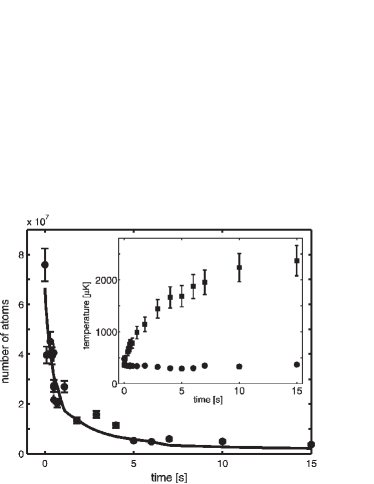
Figure 4: Decay measurement using method (i). The number of atoms $N_{3}$(t) remaining in the $m_{S}=3$ state after a variable free evolution time in the trap at an offset field of $27$ G is depicted. The curve represents a fit using the solution of Eq. 17. The inset provides the temperature evolution with (bullets) and without (squares) rf-shield.

The fit to a two body decay using the solution of Eq. (17) yields $\beta_{dr}=(2.5\,\pm\,0.5)\cdot 10^{11}\,cm^{3}/s$ and is indicated by the black curve in the figure. The inset to this figure demonstrates the evolution of the temperature with (bullets) and without (squares) rf-shield. Hereby, the temperature is derived from the width of the cloud. Without rf-shield, strong heating with an initial rate of more than 600 $\mu$K/s is observed. With rf-shield, the temperature remains constant.

The results of the decay measurements are summarized in Fig. 5. The scatter of the data for a given offset field indicates the uncertainty in our measurement. As expected, the loss coefficient increases with increasing field. Each bullet represents a separate decay measurement. Also included are two values (depicted by open squares), which were measured in a different experimental setup using the same method. The diamonds which are linked by a straight lines to guide the eye, represent the results obtained from the theoretical model using Eq. (18) and the experimental parameters $T$ and $B_{0}$. Though there is a slight discrepancy between the data and the model calculation, the experimental values are reproduced within a factor of two.

Figure 5: Dependence of the dipolar rate constant $\beta^{\circ}_{dr}$ on the offset field $B_{0}$. Depicted are $\beta^{\circ}_{dr}$ (bullets), the calculated values (diamonds, connected by straight lines to guide the eye) and values obtain from a different setup (open squares). The calculated values are obtained by using Eq. (18) and the experimental parameters $T$ and $B_{0}$

.

The deviation between the two experimental data sets is attributed to systematic errors in the determination of the density in these experiments.

Measurements of the dipolar relaxation rate at low offset fields have been performed using method (ii). Fig. 6 shows a typical result of a Stern-Gerlach Experiment at an offset field of $0.7$ G. The figure contains the evolution of the number of atoms in each sub-level and the total number of atoms ($N_{tot}(t)=N_{1}(t)+N_{2}(t)+N_{3}$(t)) during the first $15$ s. While the total number of trapped atoms (circles) stays approximately constant, about 35% of the atoms initially in the $m_{S}=3$ state (squares) get redistributed among the other trapped states.

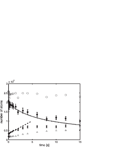
Figure 6: Redistribution among the sub-levels. While the total number of atoms ($N_{tot}$)(circles) stays constant, the population of the initially almost polarized sample gets redistributed by dipolar relaxation and spin exchange collisions. The population $N_{mS}$ of each sub-levels $m_{S}=1,2$ and $3$ is indicated by triangles, diamonds and squares, respectively. Also shown are the fitting curves to the decay of the $m_{S}=3$ (dotted line) and loading of the $m_{S}=2$ state (dashed line).

The initially prepared atomic cloud is not fully polarized even at $t=0$ s. We observe a small fraction of the cloud (about 20%) in the $m_{S}=1,2$ states (triangles, diamonds). The origin of this population remains unclear and might either be caused by incomplete rf evaporation or by Majorana spin flips Petrich1995 during switching of the magnetic fields. An indication that evaporative cooling populates these states is the slightly decreasing number of atoms which can be observed in the first few hundred ms in the $m_{S}=1,2$ states in samples with lower densities.

The decay of the $m_{S}=3$ population is non-exponential. The dynamics is described by two coupled, non-linear differential Eqs. (19) and (21) (where $\overline{V}(t)\propto\linebreak T^{3/2}(t)$). By assuming a linear increase in the volume which is describing by our data well, we obtain a solution for Eq. (19). A fit to data for which the population of the $m_{S}=2$ state is below $25\%$ yields a dipolar relaxation rate constant of $\widetilde{\beta}_{dr}=(3.1\,\pm\,0.4)\cdot 10^{-12}$ cm³s^-1. The fit to N₃(t) is illustrated by a dotted curve. We repeated this measurement for 5 different offset fields ranging from $0.15$ to $1.7$ G. The dependence of the measured values on the offset field is shown in Fig. 7. Again, the diamonds which are connected by straight lines to guide the eye are obtained from Eq. (20) using the measured experimental parameters $B_{0}$ and $T$ with no other adjustable parameter.

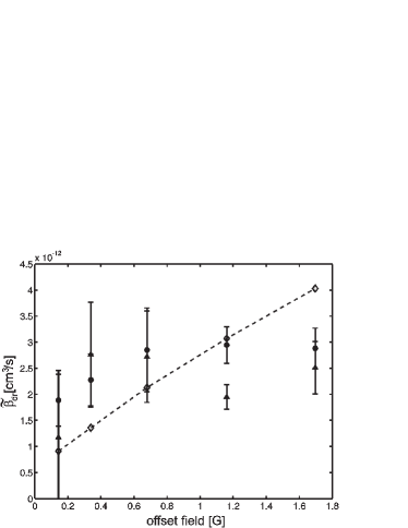
Figure 7: Dependence of the dipolar relaxation rate $\widetilde{\beta}_{dr}$ on the offset field $B_{0}$ at low magnetic fields. The experimental values obtained by method (ii) are indicated by bullets. The diamonds connected by straight lines to guide the eye are calculated using Eq. (20) and experimental parameters $B_{0}$ and T. Also included are the values (triangles) obtained from the temperature increase of the sample.

The agreement of the calculated values with the experimental data is reasonable, although the square root dependence of the decay rate on the magnetic field is not exactly reproduced.

We have also investigated the loading process of the $m_{S}=2$ state in order to deduce the two body-loss coefficient $\beta_{2}$ of this state. For short lifetimes, the loading rate into the $m_{S}=2$ state can be exclusively attributed to the loss out of the $m_{S}=3$ state. Neglecting background gas collisions, we obtain the following rate equation:

$$\frac{dN_{2}(t)}{dt}=-\frac{dN_{3}(t)}{dt}-\beta_{2}\frac{N_{2}^{2}(t)}{\overline{V}_{2}(t)}$$ (22)

where $\overline{V}_{2}=(3/2)^{3/2}\overline{V}_{3}$ is the mean volume of the thermalized $m_{S}=2$ cloud. As spin exchange collisions and dipolar relaxation are possible in this state, $\beta_{2}$ contains both processes. Assuming a constant volume, the equation can be solved. A fit of the first order power series expansion of the solution to our data yields a value of $\beta_{2}=(1.1\,\pm\,0.2)\,\cdot\,10^{-10}\,cm^{3}s^{-1}$, where we have taken the average of the measurements between $0.1$ and $1.7$ G. The fit is indicated in Fig. 6 by a dashed curve. The obtained values are shown in the inset of Fig. 7. The values of the coefficients are about a factor 50 higher than the dipolar relaxation coefficient of the $m_{S}=3$ state. This can probably be attributed to the additional decay channels mentioned in Sec.2.

We observe that the population in the $m_{S}=1$ state increases initially much slower than the population in the $m_{S}=2$ state. This indicates that $m_{S}=3$ state does not directly decay to the $m_{S}=1$ state via dipoar relaxation. The almost constant total number of atoms gives further evidence that the observed loss from the $m_{S}=3$ state involves mainly spin-flips with $\Delta m_{S}=1$. Thus, the first order Born approximation is a valid approach to describe dipolar relaxation in our system.

An example for the time evolution of the mean temperature is depicted in Fig. 8. Even at a rather low offset field of $0.7$ G the temperature of initially at $50$ $\mu$K increases rapidly with an approximate rate of $3\,\mu$K s^-1.

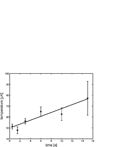
Figure 8: Heating due to dipolar relaxation at a low offset field (0.7 G). The solid line is a linear fit to the data.

We estimate the dipolar relaxation rate constant using method (iii) by solving Eq. (21) using the solution for the number of atoms in the $m_{S}=3$ state obtained above. The results of a fit to the linearized solution are included in Fig. 7 (triangles) and are in agreement with the results using method (ii).

The dipolar relaxation rate is calculated supposing that the inelastic process is dominated by the dipole-dipole interaction. Details of the molecular interaction are not taken into account. We have tested this assumption by comparing the heating of the atomic cloud due to dipolar relaxation for the two isotopes ⁵²Cr and ⁵⁰Cr. The temperature evolution of the atomic clouds at an offset field of $B_{0}=20$ G is shown in Fig. 9.

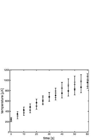
Figure 9: Heating rate due to dipolar relaxation at $20$ G offset field for the two isotopes ⁵²Cr (open circles) and ⁵⁰Cr (squares). The initial density for both isotopes is roughly $n_{0}=10^{10}$ cm^-3.

Here, the temperature was derived from the $1/\sqrt{e}$ width $\sigma_{y}$ of the cloud. Equally high heating rates ($13$ $\mu$Ks^-1) yielding the same loss coefficient can be observed for both clouds prepared with the same initial atom number density of $10^{10}$ atoms/cm³. The data shown in Fig. 9 indicate that the loss due to dipolar relaxation is independent of the details of the interatomic potential. Since the scattering length for $a(^{50}Cr)=50\,a_{0}$ and $a(^{52}Cr)=170\,a_{0}$ differs significantly Schmidt20033 one would expect that any effect due to the ’molecular’ interaction also differs for the two isotopes.

4 Conclusion

We have presented three different methods to obtain the dipolar relaxation rate constant in magnetically trapped clouds of chromium atoms. Using these methods we have measured the dependence of the rate constant on the magnetic offset field of the trapping potential. We find a typical dipolar relaxation rate constants of $\widetilde{\beta}_{dr}=4\cdot 10^{-12}$cm³s^-1 at a magnetic offset field of B${}_{0}=1$ G. Thus, even at low magnetic fields, the loss coefficient for chromium is one order of magnitude larger than the one reported for Cs in lowest hyperfine level (F=3) Guery-Odelin1998 and another 3 orders of magnitude larger than in Na Goerlitz2003 .

A theoretical estimation of the inelastic cross sections for spin-flip transitions due to the magnetic dipole-dipole interaction, predicts cross sections for single and double spin flip transition which scale with the total angular momentum to the third and second power, respectively. The values predicted by the calculation are in good agreement with the experimentally observed values. The influence of the molecular potential on the dipolar relaxation cross section for chromium was found to be insignificant.

Our findings could be especially important for experiments which aim at producing high density samples of atoms and molecules with high magnetic or electric dipole moments in magnetostatic or electrostatic traps Weinstein19981 ; Weinstein19982 ; Bethlem2000 . Large inelastic two-body collision rates are to be expected with increasing dipole-dipole interaction, if atoms are not trapped in the lowest energy state of the dipole.

As has already been pointed out in Guery-Odelin1998 dipolar relaxation can be almost totally suppressed by polarizing the sample in the energetic lowest spin state, which requires different trapping schemes. In this state neither dipolar relaxation nor spin exchange collisions are possible at reasonable offset field. The only expected loss mechanism in this case is three-body recombination. However, because of the long-range nature of the dipole potential the latter could also be increased compared to atoms with a small dipole moment. As a quite general conclusion, strong dipolar gases can only be cooled to degeneracy in traps that keep the dipole moment in its lowest energy state.

Our results, though not promising at first glance, will help us to develop a strategy for reaching Bose-Einstein condensation even under the special conditions set by the large magnetic moment of chromium. In cesium, losses due to inelastic collisions in a magnetic trap have prevented Bose-Einstein condensation for a long time in a similar way as in the chromium case. However, a careful study of the nature of the inelastic losses has finally allowed to devise a successful strategy for condensation Weber2003 .

This work was supported by the Deutsche Forschungsgemeinschaft and the RTN network ’Cold Quantum Gases’.

References

- (1) M. Baranov, L. Dobrek, K. Góral, L. Santos, M. Lewenstein: Phys. Scripta T102, 74 (2002)and reference therein
- (2) K. Góral, L. Santos, M. Lewenstein: Phys. Rev. Lett. 88, 170406 (2002)
- (3) H. Pu, W. Zhang, P. Meystre: Phys. Rev. Lett. 87, 140405 (2001)
- (4) H. Pu, W. Zhang, P. Meystre: Phys. Rev. Lett. 87, 0904001(2002)
- (5) K. Góral, K. Rza̧żewski, T. Pfau: Phys. Rev. A 61, 051601 (2000)
- (6) S. Yi, L. You: Phys. Rev. A 63, 053607 (2001)
- (7) S. Giovanazzi, A. Görlitz, T. Pfau: Phys. Rev Lett. 89, 130401 (2002)
- (8) G.V. Shlyapnikov, J.T.M. Walraven, U.M.Rahmanov, M.W. Reynolds: Phys. Rev. Lett. 73, 3247 (1994).
- (9) P.O.Fedichev, M.W. Reynolds, U.M. Rahmanov, G.V. Shlyapnikov: Phys. Rev. A 53, 1447 (1996).
- (10) D. Guéry-Odelin, J. Söding, P. Desbiolles, J. Dalibard: Europhys. Lett. 44(1), 25-30 (1998)
- (11) P.O. Schmidt, S. Hensler, J.Werner, T. Binhammer, A. Görlitz, T. Pfau: J. Opt. Soc. Am. B 20(5), 960 (2003)
- (12) P.O. Schmidt, S. Hensler, J.Werner, A. Griesmaier, A. Görlitz, T. Pfau, A. Simoni: arXiv:quant-ph/0303069 v2
- (13) P.O. Schmidt, S. Hensler, J.Werner, T. Binhammer, A. Görlitz, T. Pfau: J. Opt. B 5, S170 (2003)
- (14) N. Masuhara, J. Dolye, J.C. Sandberg, D. Kleppner, T.J. Greytak, H.F. Hess, G.P. Kochanski: Phys. Rev. Lett. 61, 935 (1988)
- (15) W. Petrich, M.H. Anderson, J.R. Ensher, E.A. Cornell: Phys. Rev. Lett. 74, 3352 (1995)
- (16) A. Görlitz, T.L. Gistavson, A.E. Leanhardt, R. Löw, A.P. Chikkatur, S. Gupta, S. Inouye, D.E Pritchard, W. Ketterle: Phys. Rev. Lett. 90, 090401 (2003)
- (17) J.D. Weinstein, R. deCarvalho, J. Kim, D. Patterson, B. Friedrich, J.M. Doyle: Phys. Rev. A 57, R3173 (1998)
- (18) J.D. Weinstein, R. deCarvalho, T. Guillet, B. Friedrich, J.M. Doyle: Nature 395, 148 (1998)
- (19) H.L. Bethlem, G. Berden, F.M.H Crompvoets, R.T. Jongma, A.J.A. van Rolj, G. Meijer: Nature 406, 491 (2000)
- (20) T. Weber, J. Herbig, M. Mark, H.-C. Nägerl, R. Grimm: Science 299, 232 (2003)