Wehrl entropy, Lieb conjecture and entanglement monotones

Abstract

We propose to quantify the entanglement of pure states of $N\times N$ bipartite quantum systems by defining its Husimi distribution with respect to $SU(N)\times SU(N)$ coherent states. The Wehrl entropy is minimal if and only if the analyzed pure state is separable. The excess of the Wehrl entropy is shown to be equal to the subentropy of the mixed state obtained by partial trace of the bipartite pure state. This quantity, as well as the generalized (Rényi) subentropies, are proved to be Schur-concave, so they are entanglement monotones and may be used as alternative measures of entanglement.

I Introduction

Investigating properties of a quantum state it is useful to analyze its phase space representation. The Husimi distribution is often very convenient to work with: it exists for any quantum state, is non-negative for any point $\alpha$ of the classical phase space $\Omega$, and may be normalized as a probability distribution Husimi (1940). The Husimi distribution can be defined as the expectation value of the analyzed state $\varrho$ with respect to the coherent state $|\alpha\rangle$, localized at the corresponding point $\alpha\in\Omega$.

If the classical phase space is equivalent to the plane one uses the standard harmonic oscillator coherent states (CS), but in general one may apply the group–theoretical construction of Perelomov Perelomov (1986). For instance, the group $SU(2)$ leads to the spin coherent states parametrized by the sphere $S^{2}={\mathbbm{C}}{\bf P}^{1}$ Radcliffe (1971); Gilmore (1972), while the simplest, degenerated representation of $SU(K)$ leads to the higher vector coherent states parametrized by points on the complex projective manifold ${\mathbbm{C}}{\bf P}^{K-1}$ Hecht (1987); Gitman and Shelepin (1993); Gnutzmann and Kuś (1998). One may define the Husimi distribution of the $N$–dimensional pure state $|\phi\rangle$ with respect to $SU(K)$–CS for any $K\leq N$, but it is important to note that if $K=N$ any pure state is by definition $SU(N)$–coherent.

Localization properties of a state under consideration may be characterized by the Wehrl entropy, defined as the continuous Boltzmann–Gibbs entropy of the Husimi function Wehrl (1978). The Wehrl entropy admits smallest values for coherent states, which are as localized in the phase space, as allowed by the Heisenberg uncertainty relation. Interestingly, this property conjectured first by Wehrl Wehrl (1978) for the harmonic oscillator coherent states was proved soon afterwords by Lieb Lieb (1978), but the analogous result for the $SU(2)$–CS still waits for a rigorous proof. This unproven property is known in the literature as the Lieb conjecture Lieb (1978). It is known that the $SU(2)$–CS provide local minimum of the Wehrl entropy C.-T.Lee (1988), while a proof of the global minimum was given for pure states of dimension $N=3$ and $N=4$ only Scutaru (1979); Schupp (1999). A generalized Lieb conjecture, concerning the Rényi -Wehrl entropies of integer order $q\geq 2$ occurred to be easier then the original statement and its proof was given in Gnutzmann and Życzkowski (2001); Schupp (1999). It is also straightforward to formulate the Lieb conjecture for Wehrl entropy computed with respect to the $SU(K)$–coherent states Słomczyński and Życzkowski (1998); Sugita (2002), but this conjecture seems not to be simpler than the original one.

In this work we consider the Husimi function of an arbitrary mixed quantum state $\rho$ of size $N$ with respect to $SU(N)$ coherent states, and calculate both its statistical moments and the Wehrl entropy. The difference between the latter quantity and the minimal entropy attained for pure states, can be considered as a measure of the degree of mixing.

Analyzing pure states of a bipartite system it is helpful to define coherent states with respect to product groups. The Wehrl entropy of a given state with respect to the $SU(N)\times SU(N)$–CS was first considered in the original paper of Wehrl Wehrl (1979). Recently Sugita proposed to use moments of the Husimi distribution defined with respect to such product coherent states as a way to characterize the entanglement of the analyzed state Sugita (2003).

In this paper we follow his idea and compute explicitly the Wehrl entropy and the generalized Rényi–Wehrl entropies for any pure state $|\Psi\rangle$ of the $N\times N$ composite system. The Husimi function is computed with respect to $SU(N)\times SU(N)$–CS, so the Wehrl entropies achieve their minimum if and only if the state $|\Psi\rangle$ is a product state. Hence the entropy excess defined as the difference with respect to the minimal value quantifies, to what extend the analyzed state is entangled. The Wehrl entropy excess is shown to be equal to the subentropy defined by Jozsa et al. Jozsa et al. (1994). Calculating the excess of the Rényi–Wehrl entropies we define the Rényi subentropy – a natural continuous generalization of the subentropy.

Several different measures of quantum entanglement introduced in the literature (see e.g. Vedral and Plenio (1998); Vidal (2000); Horodecki (2002) and references therein) satisfy the list of axioms formulated in Vedral and Plenio (1998). In particular, quantum entanglement cannot increase under the action of any local operations, and a measure fulfilling this property is called entanglement monotone.

The non-local properties of a pure state of an $N\times N$ system has to be characterized by $N-1$ independent monotones Vidal (2000). In this work we demonstrate that $N-1$ statistical moments of properly defined Husimi functions naturally provide such a set of parameters, since they are Schur–concave functions of the Schmidt coefficients and thus are non-increasing under local operations.

II Husimi function and Wehrl entropy

Any density matrix $\varrho\in{\mathbbm{C}}^{N\times N}$ can be represented by its Husimi function $H_{\varrho}(\alpha)$, that is defined as its expectation value with respect to coherent states $|\alpha\rangle$,

$$H_{\varrho}(\alpha)=\langle\alpha|\varrho|\alpha\rangle$$ (1)

In general one may define the Husimi distribution with respect to $SU(K)$-coherent states with $2\leq K\leq N$, but most often one computes the Husimi distribution with respect to the $SU(2)$ coherent states, also called spin coherent states Radcliffe (1971); Gilmore (1972). Let us recall that any family of coherent states $\{|\alpha\rangle\}$ has to satisfy the resolution of identity

$$\int_{\Omega}d\mu(\alpha)|\alpha\rangle\langle\alpha|={\mathbbm{1}}\ ,$$ (2)

where $d\mu(\alpha)$ is a uniform measure on the classical manifold $\Omega$. In the case of the degenerated representation of $SU(K)$ coherent states Hecht (1987); Gitman and Shelepin (1993); Gnutzmann and Kuś (1998) this manifold, $\Omega_{K}=U(K)/[U(K-1)\times U(1)]={\mathbbm{C}}{\bf P}^{K-1}$, is just equivalent to the space of all pure states of size $K$. This complex projective space arises from the $K$–dimensional Hilbert space ${\cal H}_{K}$ by taking into account normalized states, and identifying all elements of ${\cal H}_{K}$, which differ by an overall phase only. In the simplest case of $SU(2)$ coherent states it is just the well known Bloch sphere, $\Omega_{2}={\mathbbm{C}}{\bf P}^{1}=S^{2}$.

Analyzing a mixed state of dimensionality $N$ we are going to use $SU(N)$ coherent states, which will be denoted by $|\alpha_{N}\rangle$. With this convention the space $\Omega$ is equivalent to the complex projective space ${\mathbbm{C}}{\bf P}^{N-1}$, so every pure state is $SU(N)$–coherent and their Husimi distributions have the same shape and differ only by the localization in $\Omega$.

The $SU(N)$ coherent states may be defined according to the general group-theoretical approach by Perelomov, by a set of generators of $SU(N)$ acting on the distinguished reference state $|0\rangle$. We are going to work with the degenerate representation of $SU(N)$ only, in which a coherent state may be parametrized by $N-1$ complex numbers $\gamma_{i}$,

$$|\alpha_{N}\rangle=|\gamma_{1},\ldots,\gamma_{N-1}\rangle:=e^{\gamma_{1}J_{1}}\cdots e^{\gamma_{N-1}J_{N-1}}|0\rangle\ ,$$ (3)

where operators $J_{i}$ may be interpreted as lowering operators Gitman and Shelepin (1993). In language of the $N$–level atom they couple the highest $N$-the level with the $i$-th one (see e.g. Gnutzmann and Kuś (1998)). In the simplest case of $SU(2)$ coherent states the reference state $|0\rangle$ is equal to the eigenstate $|j,j\rangle$ of the angular momentum’s $z$-component $J_{z}$ with maximal eigenvalue, while the lowering operator reads $J_{1}=J_{-}=J_{x}-iJ_{y}$.

To characterize quantitatively the localization of an analyzed state $\varrho$ in the phase space we compute its Husimi distribution $H_{\varrho}$ with respect to $SU(N)$–CS and analyze the moments $m_{q}$ of the distribution

$$m_{q}(\varrho)=\int_{\Omega_{N}}d\mu(\alpha)\hskip 5.69046pt\left(H_{\varrho}(\alpha)\right)^{q}\ .$$ (4)

Here $d\mu(\alpha)$ denotes the unique, unitarily invariant measure on ${\mathbbm{C}}{\bf P}^{N-1}$, also called Fubini–Study measure. The measure $d\mu$ is normalized such that for any state $\varrho$ the first moment $m_{1}$ is equal to unity, so the non–negative Husimi distribution $H_{\varrho}$ may be regarded as a phase-space probability distribution.

The definition of the moments $m_{q}$ is not restricted to integer values of $q$. However, from a practical point of view it will be easier to perform the integration for integer values of $q$. But once $m_{q}$ are known for all integer $q$, there is a unique analytic extension to complex (and therefore also real) q, as integers are dense at infinity.
Another quantity of interest is the Wehrl entropy $S_{W}$, defined as Wehrl (1978)

$$S_{W}(\varrho)=-\int_{\Omega_{N}}d\mu(\alpha)\hskip 5.69046ptH_{\varrho}(\alpha)\ln H_{\varrho}(\alpha)\ .$$ (5)

Again, performing the integration might be difficult. But if all the moments $m_{q}$ are known in the vicinity of $q=1$, one can derive $S_{W}$ quite easily. Using $\partial H^{q}/\partial q=H^{q}\ln H$, one gets

$$S_{W}(\varrho)=-\lim_{q\to 1}\frac{\partial m_{q}(\varrho)}{\partial q}\ .$$ (6)

The moments $m_{q}$ of the Husimi function allow us to write the Rényi–Wehrl entropy

$$S_{W,q}(\varrho):=\frac{1}{1-q}\ln m_{q}(\varrho)\ ,$$ (7)

which tends to the Wehrl entropy $S_{W}$ for $q\to 1$. As a Husimi function is related to a selected classical phase space, the Wehrl entropy is also called classical entropy Wehrl (1978, 1979), in contrast to the von Neumann entropy $S_{N}=-\mbox{Tr}\varrho\ln\varrho$, that has no immediate relation to classical mechanics.

In section III we consider how strongly a given state is mixed and in section IV we discuss the non-locality of bipartite pure states. For this purpose we pursue an approach inspired by the Lieb conjecture Lieb (1978), according to which the Wehrl entropy $S_{W}$ of a quantum state is minimal if and only if $\varrho$ is coherent. In order to measure a degree of mixing of a monopartite mixed state of size $N$ we therefore use the $SU(N)$ coherent state, while for the study of entanglement of a bipartite pure $N\times N$ state we use the coherent states related to the product group $SU(N)\times SU(N)$.

III Monopartite systems: mixed states

In this paragraph we will focus on mixed states $\varrho\in{\mathbbm{C}}^{N\times N}$ acting on an $N$–dimensional Hilbert space ${\cal H}_{N}$. Such a state may appear as a reduced density matrix $\varrho_{r}$, defined by the partial trace $\varrho_{r}(\Psi)=\mbox{Tr}_{A}|\Psi\rangle\langle\Psi|$ of a pure state $|\Psi\rangle\in{\cal H}_{N}\otimes{\cal H}_{N}$ of a bipartite system. One could also consider a system coupled to an environment, in which a mixed state is obtained by tracing over the environmental degrees of freedom. The von Neumann entropy $S_{N}$ quantifies, on one hand, the degree of mixing of $\varrho_{r}$, and on the other, the nonlocal properties of the bipartite state $|\Psi\rangle$.

To obtain an alternative measure of mixing of $\varrho$ we are going to investigate its Husimi function defined with respect to the $SU(N)$–CS as $H^{(1)}_{\varrho}(\alpha)=\langle\alpha_{N}|\varrho|\alpha_{N}\rangle$. The moments $m_{q}$ of the Husimi distribution can be expressed as functions of the eigenvalues $\lambda_{i}$ of $\varrho$, which in the case of a reduced state of a bipartite system coincide with the Schmidt coefficients of the pure state $|\Psi\rangle$. The derivation of the explicit result in terms of the Euler Gamma function

$$\begin{array}[]{ll}\displaystyle m_{q}=\frac{N!\Gamma(q+1)}{\Gamma(q+N)}\mu_{q,N}\hskip 28.45274pt\mbox{with}\vspace{.5cm}\\ \displaystyle\mu_{q,N}=\sum_{i=1}^{N}\frac{\lambda_{i}^{q+N-1}}{\displaystyle\prod_{j=1,j\neq i}^{N}(\lambda_{i}-\lambda_{j})}\end{array}$$ (8)

is provided in Appendix A. Performing the limit (6) we find that the Wehrl entropy $S_{W}$ equals the subentropy $Q(\varrho)$ up to an additive constant $C_{N}$,

$$S_{W}(\varrho)=Q(\varrho)+C_{N}\ .$$ (9)

The $N$-dependent constant can be expressed as

$$C_{N}=\Psi(N+1)-\Psi(2)=\sum_{k=2}^{N}1/k\ ,$$ (10)

where the digamma function is defined by $\Psi(x)=\frac{\partial\ln\Gamma(x)}{\partial x}$. The subentropy

$$Q(\varrho)=-\sum_{i=1}^{N}\frac{\lambda_{i}^{N}\log\lambda_{i}}{\displaystyle\prod_{j=1,j\neq i}^{N}(\lambda_{i}-\lambda_{j})}=:Q(\vec{\lambda})$$ (11)

was defined in an information theoretical context Jozsa et al. (1994). It is related to the von Neumann entropy $S_{N}(\varrho)$ in the sense that both quantities give the lower and the upper bounds for the information which may be extracted from the state $\varrho$ Jozsa et al. (1994). The subentropy $Q(\varrho)$ takes its minimal value $0$ for pure states with only one non vanishing eigenvalue. Therefore we define the entropy excess $\Delta S$ as

$$\Delta S(\varrho)=S_{W}(\varrho)-S_{W}(\rho_{\psi})\ ,$$ (12)

where $\rho_{\psi}$ refers to an arbitrary pure state and the Wehrl entropy of an arbitrary $N$-dimensional pure state is given by $S_{W}(\rho_{\psi})=C_{N}$. Hence the entropy excess, equal to the subentropy $\Delta S(\varrho)=Q(\varrho)$, is non negative and equal to zero only for pure states.

As a byproduct we find a bound on $S_{W}(\varrho)$. The subentropy $Q(\varrho)$ is known not to be larger than the von Neumann entropy $S_{N}$ Jozsa et al. (1994). Using this fact and (9) we find that $S_{W}(\varrho)\leq S_{N}(\varrho)+C_{N}$. As it is also known that the von Neumann entropy $S_{N}$ is not larger than the Wehrl entropy $S_{W}(\varrho)$ Wehrl (1978), we end up with the following upper and lower bound on $S_{W}(\varrho)$

$$S_{N}(\varrho)+C_{N}\geq S_{W}(\varrho)\geq S_{N}(\varrho)\ .$$ (13)

IV Bipartite systems: pure states

Let us now focus on bipartite systems described by a Hilbert space ${\cal H}$ that can be decomposed into a tensor product ${\cal H}={\cal H}_{A}\otimes{\cal H}_{B}$ of two sub-spaces. With a local unitary transformation ${\cal U}_{l}={\cal U}_{A}\otimes{\cal U}_{B}$ any pure state $|\Psi\rangle\in{\cal H}$ can be transformed to its Schmidt form Peres (1995)

$$|\Psi\rangle=\sum_{i=1}^{N}\sqrt{\lambda_{i}}|i\rangle_{A}\otimes|i\rangle_{B}\ ,$$ (14)

where $N=$min(dim ${\cal H}_{A}$,dim ${\cal H}_{B}$) and the real prefactors $\lambda_{i}$ called Schmidt coefficients are the eigenvalues of the reduced density matrix $\varrho_{r}$. Thanks to the Schmidt decomposition we can assume $\mbox{dim}\hskip 2.84544pt{\cal H}_{A}=\mbox{dim}\hskip 2.84544pt{\cal H}_{B}=N$ without loss of generality. Following an idea of Sugita Sugita (2003) we consider the question whether the Wehrl entropy of a bipartite state can serve as a measure of entanglement. He defined a coherent state $|\alpha_{2}^{(M)}\rangle$ of an $M$-partite qubit system as the tensor product of $M$ coherent states $|\alpha_{2}^{(1)}\rangle$ of single qubit systems. We generalize this approach for bipartite systems, omitting the restriction to qubits and calculate all moments and the Wehrl entropy of the respective Husimi functions. For a bipartite pure state $|\Psi\rangle\in{\cal H}$, we use the tensor product of two SU$(N)$-coherent states $|\alpha_{N}^{(2)}\rangle=|\alpha_{N}\rangle^{\otimes 2}\in{\cal H}$ to define a Husimi function. More explicitly one can write $|\alpha_{N}^{(2)}\rangle=|\alpha_{N}\rangle_{A}\otimes|\alpha_{N}\rangle_{B}$, with $|\alpha_{N}\rangle_{A}\in{\cal H}_{A}$ and $|\alpha_{N}\rangle_{B}\in{\cal H}_{B}$ (we will drop the index referring to the subsystem, wherever there is no ambiguity). Such bipartite coherent states were used already in the original paper of Wehrl Wehrl (1979).

The Husimi function $H$ of a bipartite state $|\Psi\rangle$ is then given by

$$H_{\Psi}(\alpha_{A},\alpha_{B})=\bigl{|}\langle\Psi|(|\alpha_{N}\rangle_{A}\otimes|\alpha_{N}\rangle_{B})\bigr{|}^{2}\ .$$ (15)

By definition any product state is a $SU(N)\times SU(N)$ coherent state. According to the Lieb conjecture, originally formulated for $SU(2)$ coherent states, the Wehrl entropy is minimal for coherent states Lieb (1978). Hence it is natural to expect that the Wehrl entropy

$$S_{W}(\psi)=-\int_{\Omega_{N}}d\mu_{A}(\alpha)\int_{\Omega_{N}}d\mu_{B}(\alpha)\vspace{.5cm}$$

$$H_{\Psi}(\alpha_{A},\alpha_{B})\ln H_{\Psi}(\alpha_{A},\alpha_{B})$$ (16)

provides a measure of how “incoherent” a given state is. Due to the equivalence of “coherence” and separability we expect that $S_{W}$ can also serve as an entanglement measure. In the following we discuss properties of $S_{W}$ and show that it satisfies all requirements of entanglement monotones Vedral and Plenio (1998); Vidal (2000).

There is a one-to-one correspondence between states and Husimi functions. Concerning entanglement, two different states that are connected by a local unitary transformation are considered equivalent. As by construction the moments $m_{q}$ of $H$ are invariant under local unitary transformations, they reflect this equivalence and therefore can be expected to be good quantities to characterize the nonlocal properties of a bipartite state. For a pure state $|\Psi\rangle\in{\cal H}_{A}\otimes{\cal H}_{B}$, there are $N-1$ independent moments, determining $N-1$ independent Schmidt coefficients (one coefficient is determined by the normalization). In our case the moments read

$$m_{q}=\int_{\Omega_{N}}d\mu_{A}(\alpha_{A})\int_{\Omega_{N}}d\mu_{B}(\alpha_{B})\hskip 5.69046pt\Bigl{[}H_{\Psi}(\alpha_{A},\alpha_{B})\Bigr{]}^{q},$$ (17)

where the integration is performed over the Cartesian product $\Omega_{N}\times\Omega_{N}$, being the space of all product pure states of the bipartite system. The proper normalization of $d\mu_{A}$ and $d\mu_{B}$ assures that $m_{1}=1$. The required $N-1$ monotones can be provided by $m_{q}$ with $q=2,\ldots,N$. The moments can be expressed as a function of the Schmidt coefficients $\lambda_{i}$, defined in eq (14)

$$m_{q}=\left(\frac{N!\Gamma(q+1)}{\Gamma(q+N)}\right)^{2}\mu_{q,N}$$ (18)

and are related to the monopartite moments (eq. 8) by a multiplicative factor. The derivation of this result is provided in Appendix A. Having closed expressions for the moments that can be extended to real $q$, one easily finds the bipartite Wehrl entropy

$$S_{W}(\psi)=-\int_{\Omega_{N}}d\mu_{1}(\alpha_{A})\int_{\Omega_{N}}d\mu_{2}(\alpha_{B})$$

$$H_{\Psi}(\alpha_{A},\alpha_{B})\ln H_{\Psi}(\alpha_{A},\alpha_{B})\ .$$ (19)

Performing the limit (6) one finds that $S_{W}$ equals the corresponding monopartite quantity up to an additive constant

$$S_{W}(\Psi)=Q(\vec{\lambda})+2C_{N}\ .$$ (20)

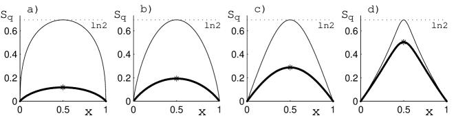
Figure 1: Rényi entropy $S_{q}$ (thin line) and Rényi subentropy $Q_{q}$ (thick line) line for the $N=2$ probability vectors as a function of the one independent variable $x$ for $q=1/2$ (a), $q=1$ (b), $q=2$ (c) and $q=10$ (d). The maximum of the Rényi subentropy is increasing with $q$ whereas the maximum of the Rényi entropy is independent of $q$. In the limit $q\to\infty$ both quantities converge to $-\ln\lambda_{max}$, where $\lambda_{max}$ is the largest component of the vector $\vec{\lambda}$.

The subentropy $Q(\lambda)$ takes its minimal value $0$ if and only if a given state is separable, i.e. if all but one Schmidt coefficients vanish. Therefore we define the bipartite entropy excess $\Delta S_{W}(\Psi)$

$$\Delta S_{W}(\Psi)=S_{W}(\Psi)-S_{W}(\phi_{sep})=Q(\varrho_{r})$$ (21)

that is vanishing if and only if $|\Psi\rangle$ is separable. Furthermore, one can also consider the Rényi–Wehrl entropy $S_{RW}^{(q)}=\frac{1}{1-q}\ln m_{q}$.

In order to use the moments $m_{q}$ as entanglement monotones, it is conventional to rescale them such that they vanish for separable states and are positive for entangled ones

$$M_{q}=\frac{1}{1-q}(\mu_{q,N}-1)\ .$$ (22)

These quantities are analogous to the Havrda-Charvat entropy (also called Tsallis entropy) Havrda and Charvat (1967); Tsallis (1988) and in the limit $q\to 1$ one obtains the subentropy

$$\lim_{q\to 1}M_{q}=Q(\vec{\lambda})\ .$$ (23)

V Rényi subentropy

As discussed in previous sections, the excess of the Wehrl entropy $\Delta S$ may be used as a measure of the degree of mixing for monopartie states, or degree of entanglement for pure states of bipartite systems. Since the moments of the Husimi distribution are found, we may extend the above analyzis for the Rényi–Wehrl entropy $S_{W,q}$ defined by (7).

Considering, for instance, the case of mixed states of a monopartite system we use (8) to find the minimal Rényi–Wehrl entropy attained for pure states $\varrho_{\psi}$,

$$C_{N,q}=S_{W,q}(\varrho_{\psi})=\frac{1}{1-q}\ln\frac{N!\Gamma(q+1)}{\Gamma(q+N)}\ ,$$ (24)

which for $q\to 1$ reduces to (10). In an analogy to (9) we define the Rényi–Wehrl entropy excess

$$\Delta S_{W,q}(\varrho)=S_{W,q}(\varrho)-C_{N,q}\ .$$ (25)

Applying (8) it is straightforward to obtain result in terms of the eigenvalues $\lambda_{i}$ of the analyzed state $\varrho$

$$\Delta S_{W,q}(\varrho)=\frac{1}{1-q}\ln\sum_{i=1}^{N}\frac{\lambda_{i}^{q+N-1}}{\displaystyle\prod_{j=1,j\neq i}^{N}(\lambda_{i}-\lambda_{j})}=:Q_{q}({\vec{\lambda}})\ .$$ (26)

This result shows that the excess of the Rényi Wehrl entropy $Q_{q}(\varrho)=Q_{q}({\vec{\lambda}})$ may be called Rényi subentropy since for $q\to 1$ it tends to the subentropy (11). On one hand it may be treated as a function of an arbitrary quantum state $\varrho$, on the other it may be defined for an arbitrary classical probability vector $\vec{\lambda}$.

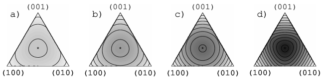
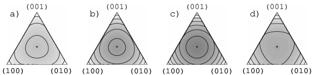
Figure 2: Rényi subentropy $Q_{q}$ as a function of two independent variables of the $N=3$ probability distributions, $q=1/2$ (a), $q=1$ (b), $q=2$ (c) and $q=5$ (d). Gray scale is used to represent the values of subentropy: the higher $q$ the larger the maximum of $Q_{q}$ at the center ${\vec{\lambda}_{*}}=(1/3,1/3,1/3)$, which refers to maximally entangled states.

Figure 3: Rescaled moments $M_{q}$ as a function of two independent variables for $N=3$ probability vectors, $q=1/2$ (a), $q=1$ (b), $q=2$ (c) and $q=5$ (d). Labels at corners identify pure separable states. Note that in general $M_{q}$ is not a monotonically increasing function of q.

In a sense $Q_{q}$ is a quantity analogous to the Rényi entropy $S_{q}$, which may be defined for an arbitrary probability vector

$$S_{q}(\vec{\lambda})=\frac{1}{1-q}\ln\sum_{i=1}^{N}\lambda_{i}^{q}.$$ (27)

In the case of quantum states $S_{q}$ is defined as a function of the $q$-th moment of the respective state

$$S_{q}(\varrho)=\frac{1}{1-q}\ln(\mbox{Tr}\varrho^{q}).$$ (28)

In the following we will sketch some properties of $Q_{q}(\vec{\lambda})$ as a function of a classical propability vector. All the considerations are also applicable in the quantum case, particularly if we use $Q_{q}$ as an entanglement monotone using the moments discussed in the preceding section. Let us define two distinguished propability vectors which correspond to extreme cases: $\vec{\lambda}_{\ast}$ with $\lambda_{i}^{\ast}=\frac{1}{N}$ ($i=1,\ldots,N$) describes the maximal random event, whereas $\vec{\lambda}_{s}$ with $\lambda_{i}^{(s)}=\delta_{i,j}$ with $j\in[1,\ldots,N]$ describes an event with a certain result. For a bipartite quantum system a vector of Schmidt coefficients given by $\vec{\lambda}_{\ast}$ represents a maximally entangled state, whereas $\vec{\lambda}_{s}$ describes a separable state.

The Rényi subentropy $Q_{q}({\vec{\lambda}})$ has the following properties

• $Q_{q}({\vec{\lambda}}_{s})=0$ for any $q$.

• $Q_{q}$ takes its maximal value $Q_{q}^{max}=\frac{1}{1-q}\ln\frac{\Gamma(q+N)}{\Gamma(q+1)N!}\frac{1}{N^{q}}$ for $\vec{\lambda}_{\ast}$. For $q\to 1$ one has $Q_{q}^{max}=C_{N}-\ln N$.

• As $m_{0}^{(1)}=1$ one immediately has $\lim_{q\to 0}Q_{q}(\vec{\lambda})=0$ for any vector $\lambda$.

• For $q\to 1$ one obtains the regular subentropy, $\lim_{q\to 1}Q_{q}({\vec{\lambda}})=Q({\vec{\lambda}})$.

• For $q\to\infty$ one gets $\lim_{q\to\infty}Q_{q}({\vec{\lambda}})=-\ln\lambda_{max}$, where $\lambda_{max}$ is the largest entry of $\lambda$. Hence this limit coincides with the limit $q\to\infty$ of the Rényi entropy $S_{q}(\vec{\lambda})$.

• $Q_{q}$ is expansibile, i.e. it does not vary if the probability vector $\vec{\lambda}$ is extended by zero, $Q_{q}(\lambda_{1},\dots,\lambda_{N})=Q_{q}(\lambda_{1},\dots,\lambda_{N},0)$.

A discrete interpolation between the subentropy $Q$ and the Shannon entropy $S$ was recently proposed in Nichols and Wootters (2003). Note that a continuous interpolation between these quantities may be obtained by the Rényi subentropy $Q_{q}$ for $q$ increasing from unity to infinity combined with the Rényi entropy $S_{q}$ for $q$ decreasing from infinity to unity. It is well known Beck and Schlögl (1993) that the Rényi entropy $S_{q}$ is both a non-increasing function of $q$ and convex with respect to $q$.

We conjecture that the Rényi subentropy has opposite properties: it is non–decreasing as a function of $q$ and it is concave with respect to $q$. See Fig. 4 for some exemplary cases. Fig. 1 presents both quantities for $N=2$, while Fig. 3 and Fig. 3 present the curves of isoentropy $Q_{q}$ and equal moments $M_{q}$ obtained for $N=3$.

VI Schur concavity

So far we defined rescaled moments, Rényi entropy and Rényi subentropy. All these quantities are constructed in such a way that they are vanishing exactly for separable states. In order to legitimately use these quantities as entanglement monotones, we still have to show, that they are non increasing under local operations and classical communication, or analogously that they are Schur concave Nielsen (1999); Vidal (2000), i.e.

$$\vec{\lambda}\prec\vec{\xi}\hskip 14.22636pt\Rightarrow\hskip 14.22636pt\Delta S_{W}(\vec{\lambda})\geq\Delta S_{W}(\vec{\xi})\ ,$$ (29)

or equivalently for the other considered quantities. The expression $\vec{\lambda}\prec\vec{\xi}$ means that $\vec{\lambda}$ is majorized by $\vec{\xi}$, i.e. the components of both vectors listed in increasing order satisfy $\sum_{i=1}^{j}\lambda_{i}\leq\sum_{i=1}^{j}\xi_{i}$ for $0<j\leq N$. In order to be Schur concave, $\Delta S_{W}(\vec{\lambda})$ has first to be invariant under exchange of any two arguments, which is obviously the case, and second it has to satisfy Ando (1989)

$$(\lambda_{1}-\lambda_{2})\left(\frac{\partial\Delta S_{W}}{\partial\lambda_{1}}-\frac{\partial\Delta S_{W}}{\partial\lambda_{2}}\right)\leq 0\ .$$ (30)

For convenience we will first consider $\mu_{q,N}$. Once we know about Schur convexity or Schur concavity of $\mu_{q,N}$ one can easily deduce Schur concavity of all the other discussed quantities. The quantities $\mu_{q,N}$ can be expressed by the following representation (see eq. 57) $\mu_{q,N}=\frac{\Gamma(q+N)}{\Gamma(q+1)}\int_{\Delta}dx(\vec{\lambda}\vec{x})^{q}$, where $dx$ is a short hand notation for $dx_{1}\ldots dx_{N}$ and the integration is performed over the simplex $\Delta$ containing all propability vectors $\vec{x}$ with $\sum_{i}x_{i}=1$. Making use of this relation and assuming $\lambda_{1}>\lambda_{2}$ without loss of generality, we obtain

$$\frac{\partial\mu_{q,N}}{\partial\lambda_{1}}-\frac{\partial\mu_{q,N}}{\partial\lambda_{2}}=\frac{\Gamma(q+N)}{\Gamma(q+1)}\int_{\Delta}dx\ (\vec{\lambda}\vec{x})^{q-1}(x_{1}-x_{2})\ .$$ (31)

The full measure of the propability simplex $\Delta$ can be divided into two symmetric parts, the first part specified by $x_{1}<x_{2}$, the second one by $x_{1}>x_{2}$. After exchanging the labels $x_{1}$ and $x_{2}$ in the second part, the first and the second part coincide and one gets

$$\frac{\partial\mu_{q,N}}{\partial\lambda_{1}}-\frac{\partial\mu_{q,N}}{\partial\lambda_{2}}=\frac{\Gamma(q+N)}{\Gamma(q+1)}\int_{\Delta_{>}}dx(x_{1}-x_{2})(\lambda_{1}-\lambda_{2})$$

$$\left(\Bigl{(}\lambda_{1}x_{1}+\lambda_{2}x_{2}+\sum_{i>2}\lambda_{i}x_{i}\Bigr{)}^{q-1}-\Bigl{(}\lambda_{1}x_{2}+\lambda_{2}x_{1}+\sum_{i>2}\lambda_{i}x_{i}\Bigr{)}^{q-1}\right)\ .$$ (32)

Since $x_{1}>x_{2}$ and $\lambda_{1}>\lambda_{2}$, one has $x_{1}\lambda_{1}+x_{2}\lambda_{2}>x_{2}\lambda_{1}+x_{1}\lambda_{2}$. Therfore for $q>1$ the integrand is non-negative and so is the integral. For $0<q<1$ the integrand is non-positive. Thus $\mu_{q,N}$ is Schur convex for $q>1$ and Schur concave for $0<q<1$. Using this, one easily concludes that

$$(\lambda_{1}-\lambda_{2})\left.\left(\frac{\partial}{\partial\lambda_{1}}-\frac{\partial}{\partial\lambda_{2}}\right)\frac{\partial\mu_{q,N}}{\partial q}\right|_{q=1}\geq 0\ .$$ (33)

As $\Delta S_{W}$ can be expressed as $\Delta S_{W}=-\lim_{q\to 1}\frac{\partial\mu_{q,N}}{\partial q}$, Schur concavity of the subentropy can directly inferred from the corresponding properties of $\mu_{q,N}$. Also the rescaled moments (22) are Schur concave for all values of $q$, as $1-q$ is negative for $q>1$ where $\mu_{q,N}$ is Schur convex.

For the Rényi subentropy $Q_{q}$ with $q\neq 1$ we have

$$(\lambda_{1}-\lambda_{2})\left(\frac{\partial Q_{q}}{\partial\lambda_{1}}-\frac{\partial Q_{q}}{\partial\lambda_{2}}\right)=$$

$$\frac{1}{1-q}\frac{1}{Q_{q}}(\lambda_{1}-\lambda_{2})\left(\frac{\partial\mu_{q,N}}{\partial\lambda_{1}}-\frac{\partial\mu_{q,N}}{\partial\lambda_{2}}\right)\ .$$ (34)

$Q_{q}$ is a positive quantity. Using Schur concavity of $\mu_{q,N}$ for $0<q<1$ and Schur convexity for $q>1$, we conclude that $Q_{q}$ is Schur concave for all positive values of $q$.

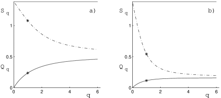
Figure 4: Rényi entropy $S_{q}$ (dashed lines) and Rényi subentropy $Q_{q}$ (solid lines) as a function of $q$ for two exemplary probability distributions. We have chosen $N=4$ probability vectors with power law distributed components, $p_{j}\propto j^{\kappa}$ with $\kappa=3/2$ in a) and $\kappa=3$ in b). Stars at $q=1$ represent Shannon entropy (upper) and subentropy (lower). We conjecture that $Q_{q}$ is both non-decreasing and concave with respect to the Rényi parameter $q$.

Since we have shown that the subentropy, the rescaled moments and the Rényi subentropy vanish if and only if the considered state is separable and that these quantities are Schur concave, these quantities are entanglement monotones and may serve as legitimate measures of quantum entanglement. Let us emphasize that the monotones found in this work differ from the Rényi entropies Życzkowski and Bengtsson (2002) and the elementary symmetric polynomials of the Schmidt coefficients Sinołȩcka et al. (2002) and cannot be represented as a functions of one of these quantities.

VII Outlook

Defining the Husimi function of a given pure state of a bi-partite $N\times N$ system with respect to coherent states related to $SU(N)\times SU(N)$ product groups and computing the Wehrl entropy allows us to establish a link between the phase space approach to quantum mechanics and the theory of quantum entanglement.

This approach may be considered as an example of a more general method of measuring the closeness of an analyzed state to a family of distinguished states. This idea, inspired by the work of Sugita Sugita (2003), may be outlined in the following set-up:

a) Consider a set of (pure or mixed) states you wish to analyze

b) Select a family of distinguished (coherent) states $|\alpha\rangle$, related to a given symmetry group and parametrized by a point on a certain manifold $\Omega$. This family of states has to satisfy the identity resolution, $\int_{\Omega}|\alpha\rangle\langle\alpha|{\rm d}\Omega={\mathbb{I}}$.

c) Define the Husimi distribution with respect to the ’coherent’ states and find the Wehrl entropy for a coherent state, $S_{min}=S(|\alpha\rangle)$

d) Calculate the Wehrl entropy for the analyzed state, $S(|\psi\rangle)$

e) Compute the entropy excess $\Delta S=S(|\psi\rangle)-S_{min}$, which characterizes quantitatively to what extend the analyzed state $|\psi\rangle$ is not ’coherent’.

For instance, analyzing the space of pure states of size $N$ we may distinguish the spin $SU(2)$ coherent states, or, in general the $SU(K)$ coherent states (with $K<N$), parametrized by a point on ${\mathbb{C}}P^{1}$ and on ${\mathbb{C}}P^{K-1}$, respectively. In the case of $N\times L$ composite quantum system we may distinguish the $SU(N)\otimes SU(L)$ coherent states. They form the set of product (separable) states and are labeled by a point on ${\mathbb{C}}P^{N-1}\times{\mathbb{C}}P^{L-1}$. For mixed states of size $N$ we may select $SU(N)$ coherent states, i.e. all pure states. In all these three cases we define the same quantity, entropy excess $\Delta S$, which has entirely different physical meaning. It quantifies the degree of non–$SU(K)$–coherence, the degree of entanglement and the degree of mixing, respectively, as listed in Table 1.

States	Mixed	Pure	Pure	Pure	Pure
Systems	simple	simple	simple	bipartite	multipartite
Coherent states	$SU(N)$ CS	$SU(2)$ CS	$SU(K)$ CS	$SU(N)\otimes SU(N)$ CS	$SU(N)^{\otimes M}$ CS
	$|\alpha_{N}\rangle\in{\mathbb{C}}P^{N-1}$	$|\alpha_{2}\rangle\in{\mathbb{C}}P^{1}$	$|\alpha_{K}\rangle\in{\mathbb{C}}P^{K-1}$	$|\alpha_{N}\rangle^{\otimes 2}\in{\mathbb{C}}P^{N^{2}-1}$	$|\alpha_{N}\rangle^{\otimes M}\in{\mathbb{C}}P^{N^{M}\!-\!1}$
Minimal Wehrl entropy	$S_{\min}=S(|\alpha_{N}\rangle)$	$S_{\min}=S(|\alpha_{2}\rangle)$	$S_{\min}=S(|\alpha_{K}\rangle)$	$S_{\min}=2S(|\alpha_{N}\rangle)$	$S_{\min}=MS(|\alpha_{N}\rangle)$
Generic states	$\rho:{\cal H}_{N}\rightarrow{\cal H}_{N}$	$|\psi\rangle\in{\mathbb{C}}P^{N-1}$	$|\psi\rangle\in{\mathbb{C}}P^{N-1}$	$|\Psi\rangle\in({\mathbb{C}}P^{N-1})^{\times 2}$	$|\Psi\rangle\in({\mathbb{C}}P^{N-1})^{\times M}$
Wehrl entropy excess $\Delta S$	$S(\rho)-C_{N}$	$S(|\psi\rangle)-C_{2}$	$S(|\psi\rangle)-C_{K}$	$S(|\Psi\rangle)-2C_{N}$	$S(|\Psi\rangle)-MC_{N}$
measures degree of	mixing	non $SU(2)$ coherence	non $SU(K)$ coherence	bi-partite entanglement	non-$M$-partite separability

Table 1: Wehrl entropy excess in various set-ups. This quantity measures the ‘distance’ of a given mixed state from the subset of pure states; the ‘distance’ of a given pure state from the subset of all $SU(K)$ coherent states; the distance of a given pure state of a composite system from the subset of all separable (product) states.

Describing the items a)–e) of the above procedure we have implicitly assumed that the Wehrl entropy is minimal if and only if the state is ’coherent’. This important point requires a comment, since the status of this assumption is different in the cases discussed. For the space of $N$–dimensional pure states analyzed by Husimi functions computed with respect to $SU(2)$ coherent states this statement became famous as the Lieb conjecture Lieb (1978). Although it was proven in some special cases of low dimensional systems Schupp (1999); Gnutzmann and Życzkowski (2001); Sugita (2002), and is widely believed to be true for an arbitrary dimensions, this conjecture still awaits a formal proof. On the other hand, it is easy to see that the Wehrl entropy of a mixed state is minimal if and only if the state is pure, or the Wehrl entropy of a bipartite pure state is minimal if and only if the state is separable. This is due to the fact that in both cases the entropy excess is equal to the subentropy which is non-negative and is equal to zero only if the state is pure Jozsa et al. (1994).

One of the main advantages of our approach is that it can easily be generalized to the problem of pure states of multipartite systems – see the last column of Table 1. It is clear that the entropy excess of $|\Psi\rangle$ is equal to zero if $|\Psi\rangle$ is a product state, but the reverse statement requires a formal proof. Moreover, the Schmidt decomposition does not work for a three (or many)–partite case. Thus in order to compute explicitly the entropy excess in these cases, one has to consider by far more terms than in the bipartite case. In the special case of three qubits any pure state may be characterized by a set of five parameters Acín et al. (2001); Sudbery (2001), and it would be interesting to express the entropy excess of an arbitrary three–qubit pure states as a function of these parameters. The second moment for this system was already calculated Sugita (2003) but expressions for other moments or for the Wehrl entropy are still missing.

VIII Acknowledgment

We are indebted to Andreas Buchleitner, Marek Kuś, Bernard Lavenda and Prot Pakoński for fruitful discussions, comments and remarks and acknowledge fruitful correspondence with Ayumu Sugita. Financial support by Volkswagen Stiftung and a research grant by Komitet Badań Narodowych is gratefully acknowledged.

Appendix A Moments of the Husimi function

As already mentioned, every pure state belonging to an $N$–dimensional Hilbert space ${\cal H}_{N}$ is a $SU(N)$ coherent state and vice versa. Therefore, following (3), we can parametrize all $SU(N)$ coherent states by

$$|\alpha\rangle=\Bigl{(}1-\sum_{i=1}^{N-1}x_{i}\Bigr{)}^{1/2}|0\rangle+\sum_{i=1}^{N-1}\sqrt{x_{i}}e^{i\varphi_{i}}|i\rangle\ ,$$ (35)

with $0\leq x_{i}\leq 1-\sum_{j=i+1}^{N-1}x_{j}$ and $d\mu=\frac{N!}{(2\pi)^{N-1}}\prod_{i=1}^{N-1}dx_{i}\hskip 2.84544ptd\varphi_{i}$. The states $|i\rangle$, ${i=0,\ldots,N-1}$ form an orthonormal basis, while $|0\rangle$ is the reference state. The Husimi function $H_{\Psi}$ of a pure state $|\Psi\rangle$ with respect to $SU(N)\otimes SU(N)$-coherent states $|\alpha_{N}^{(2)}\rangle=|\alpha_{N}\rangle_{A}\otimes|\alpha_{N}\rangle_{B}$ reads

$$H_{\Psi}=\sum_{\nu,\mu=1}^{N}\sqrt{\lambda_{\nu}\lambda_{\mu}}_{A}\langle\alpha_{N}|\nu\rangle_{A}\hskip 2.84544pt{}_{A}\langle\mu|\alpha_{N}\rangle_{A}\hskip 2.84544pt$$

$${}_{B}\langle\alpha_{N}|\nu\rangle_{B}\hskip 2.84544pt{}_{B}\langle\mu|\alpha_{N}\rangle_{B}\ ,$$ (36)

where $|\Psi\rangle$ is represented in its Schmidt basis, $|\Psi\rangle=\sum_{\nu}\sqrt{\lambda_{\nu}}|\nu\rangle_{A}\otimes|\nu\rangle_{B}$. The $q$-th moment is than given by

$$m_{q}=\sum_{{\nu_{1}...\nu_{q}=1}\atop{\mu_{1}...\mu_{q}=1}}^{N}\sqrt{\lambda_{\nu_{1}}...\lambda_{\nu_{q}}\lambda_{\mu_{1}}...\lambda_{\mu_{q}}}$$

$$f_{q}^{2}({\cal N}_{1},...,{\cal N}_{N},{\cal M}_{1},...,{\cal M}_{N})\ ,$$ (37)

with

$$f_{q}=\int d\mu(\alpha)\langle\alpha|\nu_{1}\rangle\langle\mu_{1}|\alpha\rangle\langle\alpha|\nu_{2}\rangle\langle\mu_{2}|\alpha\rangle...\langle\alpha|\nu_{q}\rangle\langle\mu_{q}|\alpha\rangle$$ (38)

The integers ${\cal N}_{i}$ and ${\cal M}_{i}$ count how often the states $|\nu_{i}\rangle$ and $\langle\mu_{i}|$ appear in $f_{q}$. Note that one has to integrate separately over both sub-systems. Due to the symmetry of the Schmidt decomposition with respect to the two subsystems, both integrations lead to the same result and it is just the square of the integral over $f_{q}$ that is entering $m_{q}$. Using the parametrization (35) $f_{q}$ can be expressed as

$$f_{q} = \frac{N!}{(2\pi)^{N-1}}\prod_{i=1}^{N-1}\int_{0}^{x_{i}^{(max)}}dx_{i}\int_{0}^{2\pi}d\varphi_{i}\hskip 5.69046pte^{i({\cal N}_{i}-{\cal M}_{i})\varphi_{i}}$$ (39)

$$x_{i}^{\frac{1}{2}({\cal N}_{i}+{\cal M}_{i})}(1-\sum_{j=1}^{N-1}x_{j})^{q-\frac{1}{2}\sum_{\chi=1}^{N-1}{\cal N}_{\chi}+{\cal M}_{\chi}}\ ,$$

where the integrations over $x_{i}$ are performed in increasing order of $i$ and the upper integration limit is given by $x_{i}^{(max)}=1-\sum_{j=i+1}^{N-1}x_{j}$. It is useful to perform the $\varphi_{i}$ integrations first. They lead to $\delta_{{\cal N}_{i},{\cal M}_{i}}$ terms, so that one gets

$$f_{q} = N!\left(\prod_{i=1}^{N-1}\int_{0}^{x_{i}^{(max)}}dx_{i}\hskip 5.69046ptx_{i}^{{\cal N}_{i}}\delta_{{\cal N}_{i},{\cal M}_{i}}\right)$$ (40)

$$(1-\sum_{j=1}^{N-1}x_{j})^{q-\sum_{\chi=1}^{N-1}{\cal N}_{\chi}}\ .$$

In order to perform the integrations over $x_{i}$ we need to define an auxiliary function

$$g_{q}(\beta,N)=\left(\prod_{i=1}^{N-1}\int_{0}^{\tilde{x}_{i}^{(max)}(\beta)}dx_{i}\hskip 5.69046ptx_{i}^{{\cal N}_{i}}\right)(\beta-\sum_{j=1}^{N-1}x_{j})^{q-\sum_{\chi=1}^{N-1}{\cal N}_{\chi}}\ ,$$ (41)

with $\tilde{x}_{i}^{(max)}(\beta)=\beta-\sum_{j=i+1}^{N-1}x_{j}$. In the following we will show that for any integer $q$

$$g_{q}(\beta,N)=\beta^{(q+N-1)}\frac{(\prod_{i=1}^{N-1}{\cal N}_{i}!)(q-\sum_{i=1}^{N-1}{\cal N}_{i})!}{(q+N-1)!}$$ (42)

holds. According to the definition (41), $g_{q}(\beta,N)$ satisfies the following relation

$$g_{q}(\beta,N)=\int_{0}^{\beta}dx_{N-1}\hskip 5.69046ptx_{N-1}^{{\cal N}_{N-1}}g_{q-{\cal N}_{N-1}}(\beta-x_{N-1},N-1)$$ (43)

Making use of

$$g_{q}(\beta,1) = \int_{0}^{\beta}dx_{1}\hskip 5.69046ptx_{1}^{{\cal N}_{1}}\hskip 2.84544pt(\beta-x_{1})^{q-{\cal N}_{1}}$$ (44)

$$= \beta^{q+1}\frac{{\cal N}_{1}!(q-{\cal N}_{1})!}{(q+1)!}\ ,$$

we immediately have (42) for $N=2$

$$g_{q}(\beta,2)=\int_{0}^{\beta}dx_{1}\hskip 5.69046ptx_{1}^{{\cal N}_{1}}(\beta-x_{1})^{q-{\cal N}_{1}}\ .$$ (45)

Assuming that (42) holds true for $g_{q}(\beta,N-1)$ and making use of (43) one gets

$$g_{q}(\beta,N) =\int_{0}^{\beta}dx_{N-1}\hskip 5.69046ptx_{N-1}^{{\cal N}_{N-1}}(\beta-x_{N-1})^{q+N-2-{\cal N}_{N-1}}$$ (46)

$$\frac{(\prod_{i=1}^{N-2}{\cal N}_{i}!)(q-{\cal N}_{N-1}-\sum_{i=1}^{N-2}{\cal N}_{i})!}{(q+N-2-{\cal N}_{N-1})!}\ .$$

Using further (44) one has

$$g_{q}(\beta,N) = \beta^{q+N-1}\frac{{\cal N}_{N-1}!(q+N-2-{\cal N}_{N-1})!}{(q+N-1)!}$$ (47)

$$\frac{(\prod_{i=1}^{N-2}{\cal N}_{i}!)(q-\sum_{i=1}^{N-1}{\cal N}_{i})!}{(q+N-2-{\cal N}_{N-1})!}\ .$$

Finally one ends up with

$$g_{q}(\beta,N)=\beta^{q+N-1}\frac{(\prod_{i=1}^{N-1}{\cal N}_{i}!)(q-\sum_{i=1}^{N-1}{\cal N}_{i})!}{(q+N-1)!}\ ,$$ (48)

i.e. (42) also holds for $g_{q}(\beta,N)$. Finally for $\beta=1$, we get

$$f_{q}=N!\frac{\left(\prod_{i=1}^{N-1}({\cal N}_{i}!)\right)\left(q-\sum_{i=1}^{N-1}{\cal N}_{i}\right)!}{(q+N-1)!}\prod_{j=1}^{N-1}\delta_{{\cal N}_{j},{\cal M}_{j}}\ .$$ (49)

Now we have $m_{q}=\sum_{\nu_{1}...\nu_{q}=1}^{N}\lambda_{\nu_{1}}...\lambda_{\nu_{q}}f_{q}^{2}$, where the $\delta_{n_{\nu},m_{\nu}}$-terms assure that there are only integer powers of the $\lambda_{\nu_{i}}$. Since $f_{q}$ depends only on the integer powers ${\cal N}_{i}$ of the $\lambda_{\nu_{i}}$, we need to count how many terms with fixed powers occur. Using simple combinatorics one can see that there are $\left(\frac{q!}{\left(\prod_{i=1}^{N-1}({\cal N}_{i})!\right)\left(q-\sum_{i=1}^{N-1}{\cal N}_{i}\right)!}\right)^{2}$ terms containing the expression $\lambda_{1}^{{\cal N}_{1}}\lambda_{2}^{{\cal N}_{2}}\ldots\lambda_{N-1}^{{\cal N}_{N-1}}\lambda_{N}^{q-\sum_{i=1}^{N-1}{\cal N}_{i}}$. Thus finally we get

$$m_{q} = \left(\frac{N!\Gamma(q+1)}{\Gamma(q+N)}\right)^{2}\sum_{{\cal N}_{1}=0}^{q}\sum_{{\cal N}_{2}=0}^{q-\nu_{1}}...\sum_{{\cal N}_{N-1}=0}^{q-\sum_{i=1}^{N-2}{\cal N}_{i}}$$ (50)

$$\lambda_{1}^{{\cal N}_{1}}\lambda_{2}^{{\cal N}_{2}}\ldots\lambda_{N-1}^{{\cal N}_{N-1}}\lambda_{N}^{q-\sum_{i=1}^{N-1}{\cal N}_{i}}\ .$$

To end, we will show by induction that for any positive integer $q$ the quantity $\mu_{q,N}$ can be written as

$$\mu_{q,N}=\sum_{{\cal N}_{1}=0}^{q}\sum_{{\cal N}_{2}=0}^{q-\nu_{1}}\ldots\sum_{{\cal N}_{N-1}=0}^{q-\sum_{i=1}^{N-2}{\cal N}_{i}}\lambda_{1}^{{\cal N}_{1}}\lambda_{2}^{{\cal N}_{2}}\ldots\lambda_{N-1}^{{\cal N}_{N-1}}\lambda_{N}^{q-\sum_{i=1}^{N-1}{\cal N}_{i}}\ .$$ (51)

As a starting point for this line of reasoning we are going to demonstrate that $\mu_{-1,N}=0$. For $N=2$ this equality can be checked by direct calculation. For $N>2$ we have

$$\mu_{-1,N} = \sum_{i=1,i\neq j}^{N}\frac{\lambda_{i}^{N-3}}{\prod_{k=1,k\neq i,k\neq j}(\lambda_{i}-\lambda_{k})}\frac{\lambda_{i}}{\lambda_{i}-\lambda_{j}}+$$ (52)

$$\frac{\lambda_{j}^{N-2}}{\prod_{k=1,k\neq j}(\lambda_{j}-\lambda_{k})}\ .$$

Since $\frac{\lambda_{i}}{\lambda_{i}-\lambda_{j}}=1+\frac{\lambda_{\alpha}}{\lambda_{i}-\lambda_{j}}$, we can make use of the following relation $\sum_{i=1,i\neq j}^{N}\frac{\lambda_{i}^{N-3}}{\prod_{k=1,k\neq i,k\neq j}(\lambda_{i}-\lambda_{k})}=\mu_{q,N-1}(\lambda_{1},\ldots,\lambda_{j-1},\lambda_{j+1},\ldots,\lambda_{N})$, in which the right hand side vanishes by assumption. Therefore we end up with

$$\mu_{-1,N}=\lambda_{j}\sum_{i=1}^{N}\frac{\lambda_{i}^{N-3}}{\prod_{k=1,k\neq i}^{N}(\lambda_{i}-\lambda_{k})}\ .$$ (53)

We still have the freedom to choose the index $j$. As the result does not depend on the choice of $j$, both sides of the equality have to be zero. Now we can come back to the proof of (51). For $N=2$ it is just a straight forward calculation to show that

$$\sum_{\nu=0}^{q}\lambda_{1}^{\nu}\lambda_{2}^{q-\nu}=\frac{\lambda_{1}^{q+1}}{\lambda_{1}-\lambda_{2}}+\frac{\lambda_{2}^{q+1}}{\lambda_{2}-\lambda_{1}}=\mu_{q,N}\ ,$$ (54)

which can be checked by multiplying both sides with $\lambda_{1}-\lambda_{2}$. Assuming that (51) is true for $N-1$ we get

$$m_{q,N}=\sum_{\nu=0}^{q}\mu_{q-\nu,N-1}\lambda_{N}^{\nu}\ .$$ (55)

Making use of the assumption (51) one obtains

$$m_{q,N} = \sum_{i=1}^{N-1}\frac{\lambda_{i}^{N-2}}{\prod_{j=1,j\neq i}^{N-1}(\lambda_{i}-\lambda_{j})}\frac{\lambda_{i}^{q+1}-\lambda_{N}^{q+1}}{\lambda_{i}-\lambda_{N}}$$ (56)

$$= \sum_{i=1}^{N}\frac{\lambda_{i}^{q+N-1}}{\prod_{j=1,j\neq i}^{N}(\lambda_{i}-\lambda_{j})}-$$

$$-\lambda_{N}^{q+1}\sum_{i=1}^{N}\frac{\lambda_{i}^{N-2}}{\prod_{j=1,j\neq i}^{N}(\lambda_{i}-\lambda_{j})}\frac{\lambda_{i}^{q+1}-\lambda_{N}^{q+1}}{\lambda_{i}-\lambda_{N}}\ .$$

Now one just has to make use of $\mu_{-1,N}=0$ and one immediately gets that the assumption (51) holds true for $N$. This result together with (50) completes the proof of Eq. (8) for integer positive integers $q$. Since integers are dense at $\infty$, we conclude that there is a unique generalisation to real $q$. Thus eq (8) is also valid for real $q$. Eq (18) for the moments of the Husimi function of a monopartite system differs by a proportionality constant only and its proof is analogous.

Appendix B Integral representation of the moments

In order to prove that

$$\mu_{q,N}=\frac{\Gamma(q+N)}{\Gamma(q+1)}\int_{\Delta}dx(\vec{\lambda}\vec{x})^{q}\ ,$$ (57)

where the integration is performed over the propability simplex $\Delta$, we consider the function $h_{q,N}(a,b)$ of two real variables $a$ and $b$ defined as

$$h_{q,N} = \frac{\Gamma(q+N)}{\Gamma(q+1)}\int_{0}^{1-a}dx_{n-1}\ldots\int_{0}^{1-a-\sum_{i>1}x_{i}}dx_{1}$$ (58)

$$(\sum_{i=1}^{n-1}x_{i}\lambda_{i}+\bigl{(}1-a-\sum_{i=1}^{n-1}x_{i})\lambda_{n}+b\bigr{)}^{q}\ .$$

Now we are going to show by induction that $h$ can be expressed as

$$h_{q,N}(a,b)=\sum_{i=1}^{n}\frac{\bigl{(}(1-a)\lambda_{i}+b\bigr{)}^{q+n-1}}{\prod_{j\neq i}(\lambda_{i}-\lambda_{j})}\ .$$ (59)

For $N=2$ it is straight forward to check that the assumption 59 holds. For $N>2$ we obtain

$$h_{q,N}=\frac{\Gamma(q+N)}{\Gamma(q+1)}\sum_{i=1}^{N-2}\frac{1}{\prod_{j\neq i}(\lambda_{i}-\lambda_{j})}\int_{0}^{1-a}dx_{N-1}$$

$$\bigl{(}(1-a-x_{N-1})\lambda_{N-1}+b+x_{N-1}\lambda_{N-1}\bigr{)}^{q+N-2}\ ,$$ (60)

where we were using the assumtion for $h_{q,N-1}(a+x_{n-1},b+x_{n-1}\lambda_{n-1}$. Performing the integration one gets

$$h_{q,N}=\frac{\Gamma(q+N)}{\Gamma(q+1)}\left(\sum_{i=1}^{N-2}\frac{\bigl{(}(1-a)\lambda_{i}+b\bigr{)}^{q+n-1}}{\prod_{j\neq i}(\lambda_{i}-\lambda_{j})}+\right.$$

$$\left.\sum_{i=1}^{N-2}\frac{\bigl{(}(1-a)\lambda_{N-1}+b\bigr{)}^{q+n-1}}{(\lambda_{N-1}-\lambda_{i})\prod_{j\neq i}(\lambda_{i}-\lambda_{j})}\right)$$ (61)

We are done, if we manage to show that

$$\sum_{i=1}^{N-2}\frac{1}{(\lambda_{N-1}-\lambda_{i})\prod_{j\neq i}^{N-2}(\lambda_{i}-\lambda_{j})}=$$

$$\frac{1}{\prod_{j=1}^{N-1}(\lambda_{N-1}-\lambda_{j})}\ ,$$ (62)

or eqivalently

$$p=\sum_{i=1}^{N-2}\prod_{j\neq i}^{N-2}\frac{\lambda_{N-1}-\lambda_{j}}{\lambda_{i}-\lambda_{j}}=1\ .$$ (63)

This is a polynomial of $(N-2)$-nd order in $\lambda_{N-1}$. If we find $N-1$ different values for $\lambda_{N-1}$ such that $p$ equals $1$, the polynomial $p$ has to be identically equal to unity. Inserting $\lambda_{k}$ ($k=1,\ldots,N-1$) one gets

$$p=\prod_{j\neq k}\frac{\lambda_{k}-\lambda_{j}}{\lambda_{k}-\lambda_{j}}=1$$ (64)

Thus $p\equiv 1$, which completes the proof of eq. (59). Setting $a=b=1$ in eq. (58) and eq. (59), we immeadiately get eq. (57).

References

• Husimi (1940) K. Husimi, Proc. Phys. Math. Soc. Jpn. 22, 264 (1940).
• Perelomov (1986) A. Perelomov, Generalized Coherent States and their Applications (Springer, Berlin, 1986, 1986).
• Radcliffe (1971) J. M. Radcliffe, J. Phys. A 4, 313 (1971).
• Gilmore (1972) R. Gilmore, Ann. Phys. 74, 391 (1972).
• Hecht (1987) K. T. Hecht, The Vector Coherent State Method and its Application to Problems of Higher Symmetry (Springer, Berlin, 1987), lecture Notes in Physics 290.
• Gitman and Shelepin (1993) D. M. Gitman and A. L. Shelepin, J. Phys. A 26, 313 (1993).
• Gnutzmann and Kuś (1998) S. Gnutzmann and M. Kuś, J. Phys. A 31, 9871 (1998).
• Wehrl (1978) A. Wehrl, Rev. Mod. Phys. 50, 221 (1978).
• Lieb (1978) E. H. Lieb, Comm. Math. Phys. 62, 35 (1978).
• C.-T.Lee (1988) C.-T.Lee, J. Phys. A 21, 3749 (1988).
• Schupp (1999) P. Schupp, Comm. Math. Phys. 207, 481 (1999).
• Scutaru (1979) H. Scutaru (1979), preprint FT-180 (1979) Bucharest, and preprint arXiv math-ph/9909024.
• Gnutzmann and Życzkowski (2001) S. Gnutzmann and K. Życzkowski, J. Phys. A 34, 10123 (2001).
• Słomczyński and Życzkowski (1998) W. Słomczyński and K. Życzkowski, Phys. Rev. Lett. 80, 1880 (1998).
• Sugita (2002) A. Sugita, J. Phys. 35, L621 (2002).
• Wehrl (1979) A. Wehrl, Rep. Math. Phys. 16, 353 (1979).
• Sugita (2003) A. Sugita, J. Phys. A 36, 9081 (2003).
• Jozsa et al. (1994) R. Jozsa, D. Robb, and W. K. Wootters, Phys. Rev. A 49, 052302 (1994).
• Vedral and Plenio (1998) V. Vedral and M. B. Plenio, Phys. Rev. A 57, 1619 (1998).
• Vidal (2000) G. Vidal, J. Mod. Opt. 47, 355 (2000).
• Horodecki (2002) M. Horodecki, Quant. Inf. Comp. 1, 3 (2002).
• Peres (1995) A. Peres, Quantum Theory: Concepts and Methods (Kluver, Dodrecht, 1995).
• Havrda and Charvat (1967) J. Havrda and F. Charvat, Kybernetica 3, 30 (1967).
• Tsallis (1988) C. Tsallis, J. Stat. Phys. 52, 479 (1988).
• Nichols and Wootters (2003) S. R. Nichols and W. K. Wootters, Quant. Inf. Comp. 3, 1 (2003).
• Beck and Schlögl (1993) C. Beck and F. Schlögl, Thermodynamics of Chaotic Systems (Cambridge University Press, Cambridge, 1993).
• Nielsen (1999) M. A. Nielsen, Phys. Rev. Lett. 83, 436 (1999).
• Ando (1989) T. Ando, Linear Algebra Appl. 118, 163 (1989).
• Życzkowski and Bengtsson (2002) K. Życzkowski and I. Bengtsson, Ann. Phys. (N.Y.) 295, 115 (2002).
• Sinołȩcka et al. (2002) M. Sinołȩcka, K. Życzkowski, and M. Kuś, Acta Phys. Pol. B 33, 2081 (2002).
• Acín et al. (2001) A. Acín, A. Andrianov, E. Jané, and R. Tarrach, J. Phys. A 34, 6725 (2001).
• Sudbery (2001) A. Sudbery, J. Phys. A 34, 643 (2001).