Analysis of the loss of coherence in interferometry with macromolecules

Abstract

We provide a self-contained quantum description of the interference produced by macromolecules diffracted by a grating, with particular reference to fullerene interferometry experiments arnzei99 ; JMO2000 . We analyze the processes inducing loss of coherence consisting in beam preparation (collimation setup and thermal spread of the wavelengths of the macromolecules) and in environmental disturbances. The results show a good agreement with experimental data and highlight the analogy with optics. Our analysis gives some hints for planning future experiments.

I Introduction

The aim of this paper is to provide a theoretical derivation of the measured beam intensity profile for interferometry with macromolecular beams, under the influence of the processes inducing loss of coherence, consisting both in beam preparation (collimation setup and thermal spread of the wavelengths of the macromolecules) and in environmental disturbances.

We have been motivated by the impressive experiments with fullerene made by Zeilinger’s group arnzei99 ; JMO2000 . In these experiments, thermally produced beams of heavy macromolecules are collimated, diffracted by a grating and then detected on a distant screen. The diffraction pattern so produced shows the typical interference profile of wave phenomena in the presence of incoherent contributions, and the reduced fringe visibility observed reminds very much of Kirchhoff diffraction with thermal light produced by an extended source. By taking into account the effects of the interaction of the macromolecules with the environment and with the photons they emit by internal cooling, we shall provide a self-contained quantum description of these experiments, that does not rely on methods of classical optics.

Our analysis is based on two main ingredients. The first one is a matter of principle: it is the formula for the statistics of particle arrival position and time on a distant surface given by Eq. (1) below. According to this formula, the intensity pattern revealed on a distant screen can be expressed in terms of the large-distance asymptotic behavior of the time-integrated quantum current (see Eq. (3) below). This formula was conjectured long time ago within the framework of scattering theory Combes , and only recently has been derived nino2 ; det2 ; det3 , extended to the mesoscopic regime, and physically motivated within the framework of Bohmian mechanics nino .

The second ingredient is a matter of analysis to simplify the dynamics of a test particle moving in a quantum medium: it is the model of Joos and Zeh joze85 for the phenomenological description of processes inducing loss of coherence in quantum systems. In this model, the reduced density matrix of the system evolves autonomously according to a “Boltzmann-type” master equation. The effect of the environment is summarized by “a collision term”, added to the free dynamics of the system, which takes into account the decoherence, i.e., damping of the off-diagonal terms of the density matrix in position representation.

Starting from these premises, and by means of some approximations that are reasonable in the common experimental conditions for interferometry with heavy particles, we shall derive an easy relation useful to describe diffraction patterns.

Finally, we shall provide a theoretical fit for the experimental data reported in JMO2000 , and we shall discuss some predictions about the dependence of the interference patterns on physical parameters such as the mass of the molecules, the pressure at which the experiment is performed and the distance of the detection screen. These predictions can be of some relevance for planning new experiments.

II Measured Intensity

In the experiments with fullerenes a thermally produced beam of heavy macromolecules is collimated, diffracted by a grating and then detected on a distant screen (see Fig. 1). The grating is composed by parallel slits, and it is periodic of period $D$. The grating and the detection screen lie in parallel planes, which are orthogonal to the longitudinal direction of beam propagation ($y$ direction), the so-called optical axis. The screen is placed at the distance $L$ from the grating. During the flight from the grating to the screen the fullerenes interact with air at low pressure, as well as with thermal photons, and get entangled with the photons emitted by relaxation of the internal excited states. What is the theoretical prediction for the particle intensity measured at the screen? In order to answer to this question we shall proceed in two steps: firstly, in Section II.1, we shall consider the case in which the dynamics of center of mass of the diffracted particle is governed by free Schrödinger evolution. Though this approximation is unrealistic for fullerenes, it is a good approximation for lighter particles as electrons or neutrons. Then, starting with Section II.2, we shall refine the description and take into account the influence of the environment on the motion of the particle.

II.1 Free evolution

In a typical detection experiment the count statistics is obtained by summing a large number of events in which the particle crosses the detection screen at a random time. What is the appropriate quantum prediction for such a statistics? This question is not quite as innocent as it sounds; it concerns in fact one of the most debated problems in quantum theory, the problem of time measurement, specifically the problem of arrival time, and position at such time. It is well known that there is no self-adjoint time observable of any sort, and since the arrival position is the position of the particle at a random time, it cannot be expressed as a Heisenberg position operator in any obvious way. Bohmian mechanics does provide, however, a remarkably simple answer (for an updated review of Bohmian mechanics see BM1 and references therein): Let $S$ be a surface in physical space, $\Psi({\bf r},t)$ be the wave function of a particle, and

$$\mathbf{J}({\bf r},t)=\frac{\hbar}{M}\,{\rm Im}\left[\Psi({\bf r},t)^{*}\>\nabla_{\bf r}\Psi({\bf r},t)\right]$$

be the associated quantum current satisfying the continuity equation

$$\frac{\partial|\Psi({\bf r},t)|^{2}}{\partial t}+\nabla_{\bf r}\cdot{\bf J({\bf r},t)}=0.$$

Then the joint probability $\mathsf{Prob}({\bf R}_{T}\in dS,T\in dt)$ that the particle crosses the surface element $d{\bf S}$ of the surface $S$ at the point ${\bf r}$ in the time between $t$ and $t+dt$ is given by

$$\mathsf{Prob}({\bf R}_{T}\in dS,T\in dt)={\bf J}({\bf r},t)\cdot d{\bf S}\,dt$$ (1)

provided the current positivity condition ${\bf J}({\bf r},t)\cdot d{\bf S}>0$ is satisfied (a condition on both the wave function $\Psi$ and on the surface $S$). See nino for a general derivation of this (for applications to mesoscopic physics see leavens1 ; leavens2 ; leavens3 , in this regard, see also grubl ).

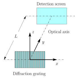
Figure 1: Geometric configuration of the diffraction grating and the detection screen.

We would like now to apply such a probabilistic prediction to the typical situation of a diffraction experiment with particles of mass $M$ diffracted by a grating and then detected on a distant screen. The geometry is that of Fig. 1 and, by (approximate) translational invariance along the slit extension—the $z$ axis—without loss of generality, we can consider the dynamics to be effectively two dimensional: ${\bf r}=(x,y)$, where $x$ is the coordinate along the grating perpendicular to the slit axes and $y$ is the coordinate perpendicular to both the grating and the detection screen, i.e., along the so-called optical axis.

Let us make the physically reasonable assumption that the initial ($t=0$) wave function produced by the grating factorizes

$$\Psi({\bf r},0)=\psi_{0}(x)\,\phi_{0}(y),$$

with the size $\Delta x$ of the support of $\psi_{0}$ being that of the grating. Then $\Psi$ evolves freely according to Schrödinger equation

$$i\hbar\frac{\partial\Psi}{\partial t}=-\frac{\hbar^{2}}{2M}{\nabla_{\bf r}}^{2}\Psi$$ (2)

until the particle is detected on the screen in the $xz$-plane placed at a “large” distance $y=L$. This last condition—see below for a suitable specification of how large $L$ should be—ensures that the current positivity condition is fulfilled. Then, according to Eq. (1), the probability density that the particle crosses the screen at the point $x$ is

$$I(x)=\left.\int^{+\infty}_{0}\!\!\!\!\!\!\!\!\mathrm{d}t\ J_{y}(x,y,t)\right|_{y=L},$$ (3)

where $J_{y}$ is the longitudinal component of the quantum current, i.e.,

$$I(x)=\frac{\hbar}{M}\int^{+\infty}_{0}\!\!\!\!\!\!\!\!\mathrm{d}t\ |\psi(x,t)|^{2}\ {\rm Im}\left[\phi(y,t)^{*}\>\frac{\partial\phi(y,t)}{\partial y}\right]_{y=L}.$$ (4)

For a large ensemble (beam) of particles identically prepared in the same initial state, by the law of large numbers, $I({x})$ is proportional to the local intensity measured at the screen—and without loss of generality, the proportionality constant, which is easily determinable by the total count statistics, will be hereafter assumed to be $1$.

Let us now make some simplifications: Assume that the momentum component $p_{y}$ is sharply defined, i.e., $\Delta p_{y}\ll p_{y}$, so that with the initial wave function is associated a well-defined de Broglie wavelength

$$\lambda\sim h/p_{y}\ll\Delta y\,.$$ (5)

Then we may approximate Schrödinger’s evolution of $\phi_{0}$ with a classical propagation at velocity $v=p_{y}/M$, so that $I(x)$ gets approximated by

$$I_{1}(x)=v\int^{+\infty}_{0}\!\!\!\!\!\!\!\!\mathrm{d}t\>\big{|}\psi({x},t)\big{|}^{2}\ \big{|}\phi_{0}\big{(}L-vt\big{)}\big{|}^{2}.$$ (6)

Suppose furthermore that the detector distance $L$ is much larger than the position spread in the longitudinal direction,

$$L\gg\Delta y.$$ (7)

Then the time-integration in Eq. (6) gives appreciable contributions only for

$$t=T\equiv\frac{L}{v}=\frac{M\lambda}{2\pi\hbar}L\,,$$ (8)

which is the so-called “time of flight,” that is the time spent by the particle to reach the detector. Thus, Eq. (6) can be further approximated as

$$I_{2}({x})=\big{|}\psi({x},T)\big{|}^{2},$$ (9)

where $\psi({x},t)$ is the solution of one-dimensional free Schrödinger’s equation, i.e.,

$$\psi(x,t)=\sqrt{\frac{M}{2\pi i\hbar t}}\int dx_{0}\>e^{\frac{iM}{2\hbar t}(x-x_{0})^{2}}\psi_{0}(x_{0})\,.$$

Consider now $|\psi(x,t)|^{2}$, i.e.,

$$\frac{M}{2\pi\hbar t}\!\iint\!\!\mathrm{d}x_{0}\,\mathrm{d}x_{0}^{\prime}\>e^{\frac{iM}{2\hbar t}[x_{0}^{2}-x_{0}^{\prime 2}+2x(x_{0}^{\prime}-x_{0})]}\>\psi_{0}(x_{0})\;\psi_{0}(x_{0}^{\prime})^{*}$$

and note that in the integrations both $x_{0}$ and $x_{0}^{\prime}$ are bounded by $\Delta x$, the support of $\psi_{0}$. Thus, if

$$\frac{M(\Delta x)^{2}}{\hbar t}\ll 1$$ (10)

we have that $e^{\frac{iM}{2\hbar t}[x_{0}^{2}-x_{0}^{\prime 2}]}\approx 1$ and therefore that $|\psi(x,t)|^{2}$ is approximated by

$$\frac{M}{2\pi\hbar t}\!\iint\!\!\mathrm{d}x_{0}\,\mathrm{d}x_{0}^{\prime}\>e^{\frac{iMx}{\hbar t}(x_{0}^{\prime}-x_{0})}\psi_{0}(x_{0})\;\psi_{0}(x_{0}^{\prime})^{*}\,.$$

One can easily recognize that the above expression (modulo an overall proportionality constant) is nothing but the square of $\widehat{\psi}_{0}(k)$, the Fourier transform of $\psi_{0}(x)$, computed for $k=Mx/(\hbar t)$. Therefore, by replacing in Eq. (9) such an approximation of $|\psi(x,t)|^{2}$ for $t=T$, and recalling definition (8) for $T$, we arrive at a further approximation for the intensity $I(x)$, namely,

$$I_{3}({x})\ =\ \frac{2\pi}{\lambda L}\ \bigg{|}\widehat{\psi}_{0}\bigg{(}\frac{2\pi{x}}{\lambda L}\bigg{)}\bigg{|}^{2}.$$ (11)

It is important to observe that the regime in which this approximation holds is that fixed by Eq. (10) for $t=T$ i.e., the regime characterized by the condition

$$\frac{\Delta x}{L}\ll\frac{\lambda}{\Delta x}\,.$$ (12)

Note that condition (12) is indeed Fraunhofer’s condition of classical optics and Eq. (11) is the corresponding formula for the intensity of classical Fraunhofer diffraction theory wolf , according to which the large-distance intensity of a diffracted field is the squared modulus of the Fourier transform of the field distribution on the diffractive grating. (For example, for a double-slit diffractive grating, with aperture $d$ of each slit, distance $D$ between the slits, and with $\psi_{0}$ being the characteristic function of the slits, Eq. (11) becomes the standard formula for the intensity in the double-slits experiment, namely,

$$\frac{I_{0}}{2}\>\mbox{sinc}^{2}\bigg{(}\frac{\pi dx}{\lambda L}\bigg{)}\,\bigg{[}1+\cos\bigg{(}\frac{2\pi Dx}{\lambda L}\bigg{)}\bigg{]}\,,$$

where $I_{0}$ is the intensity detected for $x=0$ and, as usual, $\mbox{sinc}(x)\,\equiv x^{-1}\sin(x)$.)

In this regard, it should be observed that condition (10) leading to $I_{3}(x)$ is a known condition nino ; 7steps . It corresponds to a “large time” regime

$$T\gg\tau\equiv\frac{M(\Delta x)^{2}}{\hbar}=\frac{\Delta x}{\Delta p_{x}/M}=\frac{\Delta x}{\Delta v_{x}}$$ (13)

for which the solution of Schrödinger’s equation is approximated by

$$\psi({x},t)\sim\sqrt{\frac{M}{i\hbar t}}\>e^{i\frac{M{x}^{2}}{2\hbar t}}\>\widehat{\psi}_{0}\bigg{(}\frac{M{x}}{\hbar t}\bigg{)}\,.$$

Such a wave is what in 7steps has been named “local plane wave”: a wave that locally looks like a packet, having amplitude and local wave number that are slowly varying over distances of the order of the local de Broglie wavelength. Such waves are associated with classical motion of particles and a rough estimate of the time needed for the formation of such waves is indeed the time $\tau$ above 7steps . So, evidence to the contrary notwithstanding, the particle motion in the Fraunhofer region, that is, the particle motion on the time scale (13), is indeed classical motion.

It might be useful to compare the domain of validity of the various approximations. Approximation $I_{2}(x)$ holds under the spatial condition (7), that is on the time scale

$$T\gg\frac{M\lambda}{2\pi\hbar}\Delta y\,.$$

The temporal and spatial conditions leading to the Fraunhofer-like approximation $I_{3}(x)$ are deduced by Eq. (10) for $t=T$. For an initial packet with $\Delta x\sim~{}\Delta y$, comparison of $\Delta x\ll L$ (leading to $I_{2}(x)$) with $\Delta x\ll~{}\sqrt{\lambda L}$ (leading to $I_{3}(x)$) shows that the Fraunhofer approximation is realized on much larger space and time scales.

A final remark: It could be objected that it is indeed (9) the basic formula for the statistical predictions of detection experiments—after all, it is this formula that seems to correspond directly to the standard statistical interpretation of the wave function. This objection, however, misses the point altogether: $I_{2}(x)$ is only an approximation; the time at which the particle crosses the screen is typically random, and it can be treated as the deterministic quantity given by the time of flight only when condition (7) is satisfied. In a sense, it is true that in the regime of large distances there is no experimental difference between $I(x)$ and the approximations we have considered (indeed, this is a consequence of what it has been proven with great generality in nino2 ; det3 ). However, experimental research on near field interferometry may explore regimes in which these approximations fail, e.g., when statistical fluctuations in the arrival time become experimentally relevant, as we shall comment in Section VI.3. Hence the need of an exact formula for the intensity. And, while the standard quantum formalism fails to provide the exact expression for the intensity, the formula given by Eq. (3), which clearly looks right, is naturally deduced from first principles of Bohmian mechanics nino .

II.2 Interaction with the environment

In the more general case of a quantum particle interacting with its environment, the evolution cannot be any more treated in terms of one-particle Schrödinger equation because entanglement can be fastly developed. In this case, the statistical predictions concerning experiments performed on the particle are governed by the reduced density matrix $\rho({\bf r},{\bf r}^{\prime})$, which is obtained from the wave function describing the particle and its environment by integrating out the configurational degrees of freedom of the environment; for example, for an environment with N particles and total wave function $\Psi({\bf r},{\bf r}_{1},\ldots,{\bf r}_{N})$, the reduced density matrix is given by

$$\rho({\bf r},{\bf r}^{\prime})=\!\!\int\!\mathrm{d}{\bf r}_{1}\ldots\mathrm{d}{\bf r}_{N}\Psi({\bf r},{\bf r}_{1},\ldots,{\bf r}_{N})\;\Psi({\bf r}^{\prime},{\bf r}_{1},\ldots,{\bf r}_{N})^{*}\!\!.$$ (14)

As far as detection experiments are concerned, the following natural generalization of Eq. (1) can be put forward: The joint probability that the particle crosses the surface element $d{\bf S}$ of the surface $S$ at the point ${\bf r}$ in the time between $t$ and $t+dt$ is still given by Eq. (1), but with current ${\bf J}$ given now by

$$\mathbf{J}({\bf r},t)=\frac{\hbar}{M}\,{\rm Im}\left[\nabla_{{\bf r}}\rho({\bf r},{\bf r}^{\prime},t)\right]_{{\bf r}^{\prime}={\bf r}}.$$ (15)

A detailed derivation of this result will be given elsewhere . In this regard, a key observation is that ${\bf J}$ given by Eq. (15) is indeed the right probability current entering in the continuity equation for the probability density of position $\rho({\bf r},{\bf r},t)$,

$$\frac{\partial\rho({\bf r},{\bf r},t)}{\partial t}+\nabla_{\bf r}\cdot{\bf J({\bf r},t)}=0.$$

We may now make more realistic the analysis of Section II.1 by allowing that, during the flight from the grating to the screen, the particle of mass $M$ diffracted by the grating interacts with particles of the environment (say, air molecules). As before, the geometry is that of Fig. 1, so that the dynamics is effectively two dimensional, i.e., as before, ${\bf r}=(x,y)$. Though the initial state produced by the grating needs not be anymore a pure state, we maintain the physically reasonable assumption of factorization at $t=0$,

$$\rho({\bf r},{\bf r}^{\prime},0)=\rho_{0}^{(x)}(x,x^{\prime})\rho_{0}^{(y)}(y,y^{\prime}).$$

For an environment of N particles, the time evolution of $\rho({\bf r},{\bf r}^{\prime},t)$ is that induced, according to Eq. (14), by the Schrödinger evolution of total wave function $\Psi=~{}\Psi({\bf r},{\bf r}_{1},\ldots,{\bf r}_{N},t)$,

$$i\hbar\frac{\partial\Psi}{\partial t}=-\frac{\hbar^{2}}{2M}{\nabla_{\bf r}}^{2}\Psi+H_{0}^{\text{env}}\Psi+H_{\text{int}}\Psi,$$ (16)

where $H_{0}^{\text{env}}$ is the total Hamiltonian of the $N$ particles (the sum of the kinetic and potential energies), and $H_{\text{int}}$ is the interaction potential between the particle and the other $N$ particles.

Accordingly, the exact formula for the probability density that the particle crosses the screen at the point $x$ is given by Eq. (3), where $J_{y}$ is now the longitudinal component of the probability current given by Eq. (15). We shall now simplify the expression for the intensity, in analogy with the treatment of Section II.1, by exploiting the typical physical conditions of interference experiments.

Motion along the $y$ direction is typically “very fast,” being characterized by a “very short” wavelength $\lambda$, much smaller than all the other relevant lengths scales (such as the spreads $\Delta x$, $\Delta y$, and the screen distance $L$). Accordingly, we have an effective preservation of the factorization of the initial state, and Eq. (3) becomes

$$I(x)\sim\frac{\hbar}{M}\int^{+\infty}_{0}\!\!\!\!\!\!\!\!\mathrm{d}t\ \rho^{(x)}(x,x,t)\ {\rm Im}\bigg{[}\partial_{y}\rho^{(y)}(y,y^{\prime},t)|_{y^{\prime}=y}\bigg{]}_{y=L}.$$

Note that, due to the condition of fast motion along $y$ direction, we may assume wave-packet motion, i.e., $\rho^{(y)}(y,y^{\prime},t)=\phi(y,t)\;\phi(y^{\prime},t)^{*}$, and consider the evolution of the wave packet $\phi$ to be classical. Thus, proceeding as in Section II.1 in going from Eq. (4) to Eq. (9), and a part from a caveat we shall discuss below, we arrive at the following approximation for the measured intensity

$$I_{2}(x)=\rho^{(x)}(x,x,T),$$ (17)

where $T$ is, as before, the time of flight given by Eq. (8).

The caveat is the following: in the free case a crucial condition for the validity of Eq. (9) is that $\lambda\ll\Delta y$. In case of environmental interaction the momentum spread increases due to scattering events and the previous condition is no more sufficient to assure a well defined de Broglie wavelength along the longitudinal direction. An important consequence of the analysis of Section V is that interaction with the environment produces an effective reduction of the relevant length scales over which quantum coherence is preserved and this reduction is controlled by what we shall call the “coherence length” and denote by $\ell$. In general, the validity of Eq. (17) is assured by $\lambda\ll\Delta y$ and $\lambda\ll\ell$; for relevant incoherence effects, we have $\ell\lesssim\Delta y$ and thus the crucial condition becomes: $\lambda\ll\ell$.

Let us consider the case of fullerene, and let the initial state be the state at the moment of the splitting produced by the diffractive grating. It turns out that, at this time, the motion of fullerene along the $y$-direction can be described by a narrow wave packet translating with velocity $v$. In fact, according to Tab. 1, the typical de Broglie wavelength for fullerene is $\lambda\approx 10^{-12}$ m. The analysis performed in Section III.1 leads to $\ell\approx 10^{-7}$ m (see Tab. 3), whence $\lambda\ll\ell$ (and since $L\approx 1\,$m, $\Delta y\ll L$). Thus, Eq. (17) provides a good approximation for the measured intensity of fullerenes.

N.B. Eq. (17) is the basic equation of this paper. In order to avoid notational complexity, when no confusion will arise and unless otherwise stated, we shall drop all the indices and simply write $I(x)$ instead of $I_{2}(x)$ and $\rho(x,x,T)$ instead of $\rho^{(x)}(x,x,T)$.

III Markovian Approximation

In order to evaluate $I(x)$, we need to determine $\rho({\bf r},{\bf r}^{\prime},t)$, the reduced density matrix at time $t$. In general, the evolution of $\rho$ is highly non-Markovian, being the evolution induced by Eq. (16) via Eq. (14). For an environment made of a gas at low pressure we may rely on the Markovian approximation provided by the model of Joos and Zeh joze85 . We shall now recall the essential ingredients of this model and refer to literature for a thorough discussion giulini ; flega90 . (For some basic steps towards a rigorous derivation see figari ; in this regard see also andrea ; for a more general analysis of quantum Brownian motion see bassano ; bassano2 ).

This model aims at providing an autonomous evolution equation for an heavy particle moving in a gas of light particles under the approximation of negligible friction. To get a handle on the model, consider a single collision of the heavy particle, of mass $M$, with a light particle of the medium, of mass $m$. If $M\gg m$ the time scale $\tau_{s}$ of a single-scattering process is short with respect to the typical time scale $t$ of evolution of the heavy particle. Thus, Born-Oppenheimer adiabatic approximation applies, and the dynamics of the center of mass of the heavy particle can be considered as frozen in the time $\tau_{s}$. Accordingly, if $\Psi({\bf r})$ and $\chi({\bf r}_{l})$ are, respectively, the wave functions of the heavy particle and of the light particle before the collision, the wave function of the composite system after the collision is $\Psi({\bf r})\chi_{{\bf r}}({\bf r}_{l})$, where $\chi_{{\bf r}}({\bf r}_{l})$ is the outgoing wave function of the light particle, scattered off at the point ${\bf r}=(x,y,z)$. As a consequence, the final state of the heavy particle is described by the reduced density matrix $\Psi({\bf r})\,\Psi({\bf r}^{\prime})^{*}\>\langle\chi_{{\bf r}^{\prime}}|\chi_{{\bf r}}\rangle$.

For arbitrary initial density matrix $\rho({\bf r},{\bf r}^{\prime})$, and many independent individual scattering events, the variation in the time $\Delta t$ of $\rho({\bf r},{\bf r}^{\prime})$ due to collisions is then

$$\Delta\rho({\bf r},{\bf r}^{\prime})\>\sim\>-\mathcal{N}\,\Delta t\bigg{(}1-\overline{\langle{\chi_{{\bf r}^{\prime}}}|{\chi_{{\bf r}}}\rangle}\>\bigg{)}\,\rho({\bf r},{\bf r}^{\prime}),$$

where $\mathcal{N}$ is the mean number of collisions per unit of time and $\overline{\langle{\chi_{{\bf r}^{\prime}}}|{\chi_{{\bf r}}}\rangle}$ denotes the average with respect to a suitable ensemble of light particle wave functions. By taking into account also the rate of change of $\rho$ due to the free dynamics, one arrives at the master equation of Joos and Zeh:

$$\frac{\partial\rho}{\partial t}=\mathcal{L}_{0}\,\rho+\mathcal{L}_{\!I}\,\rho\,,$$ (18)

where

$$\mathcal{L}_{0}\,\rho=-\frac{i}{\hbar}[H_{0},\rho]=\frac{i\hbar}{2M}\left[\nabla^{2},\rho\right]$$

and

$$\big{(}\mathcal{L}_{\!I}\rho\big{)}({\bf r},{\bf r}^{\prime})=\>-\mathcal{N}\bigg{(}1-\overline{\langle{\chi_{{\bf r}^{\prime}}}|{\chi_{{\bf r}}}\rangle\!}\>\bigg{)}\,\rho({\bf r},{\bf r}^{\prime}).$$ (19)

III.1 Estimation of environmental coupling

Table 1: Physical parameters of fullerene experiments JMO2000 .

Mass of fullerene ${C_{60}}$:	$M\>\approx\>1.2\times 10^{-24}\,\mathrm{Kg}$
Radius of ${C_{60}}:$	$R\>\approx\>3.5\times 10^{-10}\,\mathrm{m}$
Temperature of ${C_{60}}$:	$\Theta_{F}\>\approx\>900\,\mathrm{K}$
Environmental temperature:	$\Theta_{\mathcal{E}}\>\approx\>300\,\mathrm{K}$
Mean wavelength of ${C_{60}}$:	$\lambda\>\approx 2.5\times 10^{-12}\,\mathrm{m}$
Mean time of flighta	$T\>\approx\>6\times 10^{-3}\,\mathrm{s}$
Grating–screen distance:	$L\>=\>1.25\,\mathrm{m}$
Collimator aperture:	$a\>=\>10^{-5}\,\mathrm{m}$
Effective slits width:	$d\>\approx\>3.6\times 10^{-8}\,\mathrm{m}$
Grating period:	$D\>=\>10^{-7}\,\mathrm{m}$

For a complete specification of the RHS of (18), we need to evaluate the interaction operator (19) related to the different processes inducing entanglement of $C_{60}$ with surrounding environment: scattering events (with thermal photons and air molecules) and photon emission. Such an evaluation of the interaction operator is rather standard, and can be found in the literature on the Joos and Zeh model—modulo some numerical values that we have corrected, and with the exception of our treatment of decoherence due to photon emission that is slightly different from what can be found in the literature (see, e.g., alicki ; brukner ).

III.1.1 Scattering with thermal photons

In fullerene experiment, the environmental temperature is $\Theta_{\mathcal{E}}\approx 300\,\mathrm{K}$ and thus the wavelength of thermal photon is $\lambda_{ph}=hc/(k_{\scriptsize B}\Theta_{\mathcal{E}})\approx 4.8\times 10^{-5}\,\mathrm{m}$. As we shall see in Section IV (Eqs. (36)–(37) and relative evaluation in Tab. 3), because of the incoherent preparation of the beam, we have that $|x-x^{\prime}|\lesssim\ell_{0}\approx 10^{-7}$m. Under this condition, Eq. (19) assumes the form (see joze85 ; giulini )

$$\big{(}\mathcal{L}_{\!I}\rho\big{)}(x,x^{\prime})\>=\>-\Lambda_{\rm ph}^{\!(scat)}|\,x-x\,^{\prime}|^{2}\rho(x,x^{\prime})\,$$

with

$$\Lambda_{\rm ph}^{\!(scat)}\!\!=8!\,\frac{8\,c\,a^{6}}{3}\>\bigg{|}\frac{\epsilon_{r}-1}{\epsilon_{r}+2}\bigg{|}^{2}\!\!\zeta(9)\bigg{(}\frac{2\pi}{\lambda_{ph}}\bigg{)}^{\!9}\!\!\!\approx\,2.4\times 10^{2}\,\mathrm{m}^{-2}\mathrm{s}^{-1}\!\!,$$ (20)

where the fullerene molecule has been modeled as a dielectric sphere with the dielectric constant $\epsilon_{r}\approx 4$ epsfulle and $\zeta(9)\approx 1$, with $\zeta(z)$ representing the Riemann $\zeta$ function. The previous relation has been obtained in the regime of Rayleigh scattering (since fullerene radius $R\approx 3.5\times 10^{-10}\,\mathrm{m}$ is much smaller than $\lambda_{ph}$) and by using the Planck distribution for environmental photons .

III.1.2 Scattering with air molecules.

Air molecules, with a mean mass $m_{air}\!\approx\!4.8\times 10^{-26}\,\mathrm{Kg}$, at the temperature $\Theta_{\mathcal{E}}\approx 300\,\mathrm{K}$ have a de Broglie wavelength $\lambda_{air}=h/\sqrt{2\pi m_{air}k_{\scriptsize B}\Theta_{\mathcal{E}}}\approx\,10^{-11}\,\mathrm{m}\,\ll\ell_{0}$ (see Tab. 3). Thus, assuming a Maxwell-Boltzmann distribution for air molecule velocity, it follows from the analysis performed in flega90 (Eq. (2.17)) that

$$\big{(}\mathcal{L}_{\!I}\rho\big{)}(x,x^{\prime})\>=\>\left\{\begin{array}[]{ll}\displaystyle\sigma_{\rm tot}\,P(\Theta_{\mathcal{E}})\,\sqrt{\frac{32\pi\,}{k_{\scriptsize B}\,\Theta_{\mathcal{E}}\,m_{air}}}&\displaystyle\text{for $x\,\neq\,x\,^{\prime}$}\\[14.22636pt] 0&\text{for $x\,=\,x\,^{\prime}$,}\\[5.69046pt] \end{array}\right.$$ (21)

where $P(\Theta_{\mathcal{E}})$ is the pressure at the temperature $\Theta_{\mathcal{E}}$ and $\sigma_{\rm tot}$ is the total cross section for scattering events.

In the case of fullerene experiment $P\approx 5\times 10^{-6}\,\mathrm{Pa}$ and $\sigma_{\rm tot}\approx 9\times 10^{-18}\,\mathrm{m}^{2}$ . If $F_{\rm air}(\infty)$ is the constant value assumed by $\big{(}\mathcal{L}_{\!I}\rho\big{)}(x,x^{\prime})$ for $x\neq x^{\prime}$, from Eq. (21) we get $F_{\rm air}(\infty)\>\approx\>32\,\mathrm{s^{-1}}$. In order to make a comparison between the different decoherence sources involved in diffraction experiments, we can introduce an effective localization factor $\Lambda$ also for air scattering events. Given a pair of slits at the distance $nD$ in a periodic grating of period $D$ we have

$$\Lambda_{\rm air}(n)\>=\>\frac{F_{\rm air}(\infty)}{(n\,D)^{2}}\>.$$ (22)

For adjacent slits ($n=1$) the localization factor $\Lambda_{\rm air}$ assumes its greatest value

$$\Lambda_{\rm air}(n=1)\>\approx\>3.2\times 10^{15}\,\mathrm{m^{-2}\,s^{-1}}.$$ (23)

III.1.3 Photon emission

The model of Joos and Zeh can be extended to the description of photon emission processes. In fact, also in this case, the wave function of the composite system after a single emission event is, in general, $\Psi({\bf r})\chi_{{\bf r}}({\bf r}_{l})$, where $\Psi({\bf r})$ is the initial wave function of fullerene and $\chi_{{\bf r}}({\bf r}_{l})$ is the outgoing wave function of the photon emitted in ${\bf r}$. Since emission time scale, in analogy with scattering events, is much faster than characteristic time of fullerene free dynamics, the state $|\chi_{{{\bf r}}}\rangle$, in position representation and asymptotically in time, is well described by spherical waves

$$\langle{\bf r}_{l}\,|\chi_{{{\bf r}}}\rangle\>\propto\>\frac{e^{\,i\,k\,|\,{\bf r}_{l}-{\bf r}\,|}}{|\,{\bf r}_{l}-{\bf r}\,|}\,,$$

where $k$ is the wave number of emitted photons. It follows that

$$\langle{\chi_{{\bf r}^{\prime}}}|{\chi_{{\bf r}}}\rangle\>=\>\frac{\sin(k\,|{\bf r}-{\bf r}\,^{\prime}|)}{k\,|{\bf r}-{\bf r}\,^{\prime}|}\>\equiv\>\mathrm{sinc}(k\,|{\bf r}-{\bf r}\,^{\prime}|).$$

According to Eq. (19) and assuming that fullerene diffraction can be effectively treated as a one-dimensional problem, the interaction operator for photon emission becomes

$$\big{(}\mathcal{L}_{\!I}\rho\big{)}(x,x^{\prime})\>=\>-\mathcal{N}\,\bigg{[}1-\overline{\mathrm{sinc}(k\,|x-x\,^{\prime}|)\!}\,\bigg{]}\,\rho(x,x\,^{\prime}).$$ (24)

In fullerene experiment there are essentially two channels for photon emission: the black-body radiation and the disexcitation of internal vibrational energy levels. In particular, for black-body radiation at the fullerene temperature of $\Theta_{F}\approx 900\,\mathrm{K}$, we have a mean wavelength of emitted photon equal to

$$\lambda_{em}^{(bb)}\>\approx\>1.6\times 10^{-5}\,\mathrm{m}.$$

For decays of internal energy levels it was measured a peaked infrared spectrum with the shortest wavelength kratschmer

$$\lambda_{em}^{(vib)}\>\approx\>7\times 10^{-6}\,\mathrm{m}\,.$$

In both cases it results (see Tab. 3) $\lambda_{em}\gg\ell_{0}$. This permits to simplify Eq. (24) by the expansion of the sinc-function in powers of $k\,|x-x\,^{\prime}|$. Keeping the first no-constant term, we straightly obtain

$$\big{(}\mathcal{L}_{\!I}\rho\big{)}(x,x^{\prime})\>=\>-\Lambda_{em}\,|\,x-x\,^{\prime}|^{2}\,\rho(x,x\,^{\prime}),$$

with

$$\Lambda_{\rm em}=\frac{\mathcal{N}\,\overline{k^{2}}}{6}$$

(in agreement with what obtained by Alicki alicki ).

In the following, we shall calculate the mean value $\overline{k^{2}}$ for the two different channels of photon emission.

Black-body radiation.

The probability distribution of the wave number $k$ is given by the Planck law

$$n(k)\,\mathrm{d}k\>=\>\varepsilon\,\bigg{(}\frac{\hbar\,c}{k_{\scriptsize B}\Theta_{F}}\bigg{)}^{3}\,\frac{1}{2\zeta(3)}\>\frac{k^{2}\,\mathrm{d}k}{e^{\frac{\hbar\,c}{k_{\scriptsize B}\Theta_{F}\!}\>\,k}-1},$$

where $\varepsilon\approx 4.5\times 10^{-5}$ is the emissivity of fullerene at $\Theta_{F}\approx 900$ K emit and $\zeta(3)\approx 1.2$. Then Eq. (III.1.3) becomes

$$\Lambda_{\rm ph}^{\!(bb)}\>=\>\frac{\mathcal{N}}{6}\int\mathrm{d}k\>k^{2}\>n(k)\>=\>\frac{8\pi^{2}\,\zeta(5)}{\zeta(3)}\>\frac{\mathcal{N}\,\varepsilon}{(\lambda^{(bb)}_{em})^{2}}\,,$$ (25)

with $\zeta(5)\>\approx\>1.04$.

The number of emitted photons per unit of time can be estimated as $\mathcal{N}\sim E^{(bb)}/(k_{\scriptsize B}\Theta_{F})$, where $E^{(bb)}$ is the total energy emitted per unit of time and $k_{\scriptsize B}\,\Theta_{F}\approx 0.08\,\mathrm{eV}$ represents the single photon energy. By integrating the Planck distribution, one evaluates $E^{(bb)}\!\!=~{}\varepsilon S\sigma\Theta_{F}^{4}\approx~{}16\,\mathrm{eV}/\mathrm{s}$, where $S=4\pi R^{2}$ is the total surface of fullerene macromolecules ($R\approx 3.5\times 10^{-10}\,\mathrm{m}$) and $\sigma$ is the Stefan-Boltzmann constant. It results $\mathcal{N}\approx 200\,\mathrm{coll/sec}$, and thus

$$\Lambda_{\rm ph}^{\!(bb)}\>\approx\>2.5\times 10^{9}\,\mathrm{m^{-2}\,s^{-1}}.$$ (26)

Decay of internal vibrational energy levels.

Since we lack of a model able to describe decays of internal energy levels for fullerene, we directly refer to the results of experimental spectroscopy. Since infrared spectrum shows a peaked structure, we can write

$$\Lambda_{\rm ph}^{\!(vib)}\>\equiv\>\frac{\mathcal{N}\,\overline{k^{2}}}{6}\>\lesssim\>\frac{\mathcal{N}\,(k^{*})^{2}}{6}\>\approx\>5\times 10^{13}\,\mathrm{m}^{-2}\mathrm{s}^{-1}\>,$$ (27)

where $k^{*}\approx 9\times 10^{5}\,\mathrm{m}$ is the wave number related to the most energetic spectral line (see Fig. 4 in kratschmer ) and $\mathcal{N}\approx 400\,\mathrm{coll}/\mathrm{s}$ arnzei99 .

A direct comparison between evaluation (20), (23), (26) and (27), reported in Tab. 2, shows that the main decoherence processes are scattering with air molecules (especially for adjacent slits, cf. Eq. (22)), followed by photon emission due to decay of internal vibrational energy levels.

Table 2: Sources of decoherence in the conditions of fullerene experiments arnzei99 ; JMO2000 .

Decohering event	$\Lambda\ (\mathrm{m}^{2}\mathrm{s}^{-1})$
Scattering
with thermal photons:	$\Lambda_{\rm ph}^{\!(scat)}\>\approx\>2.4\times 10^{2},$
with air molecules:	$\Lambda_{\mathrm{a}ir}\>\lesssim\>3.2\times 10^{15}.$
Photon emission
black-body radiation:	$\Lambda_{\rm ph}^{\!(bb)}\>\approx\>2.5\times 10^{9},$
decay of excited states:	$\Lambda_{\rm ph}^{\!(vib)}\>\lesssim\>5\times 10^{13}.$
Global effect:	$\Lambda\>\lesssim\>3.3\times 10^{15}.$

III.2 The effective master equation

According to the foregoing analysis, the Joos-Zeh equation (18) effectively reduces to

$$i\hbar\frac{\partial\rho}{\partial t}=[H_{0},\rho]-i\Lambda[x,[x,\rho]]$$

or, more explicitly,

$$i\hbar\frac{\partial\rho(x,x^{\prime},t)}{\partial t}=\frac{\hbar^{2}}{2M}\left(\frac{\partial^{2}}{\partial{x^{\prime}}^{2}}-\frac{\partial^{2}}{\partial{x}^{2}}\right)\rho(x,x^{\prime},t)-i\Lambda\>(x-x^{\prime})^{2}\rho(x,x^{\prime},t)$$ (28)

with

$$\Lambda\>\equiv\>\>\Lambda_{\rm air}\,+\,\Lambda_{\rm ph}\,,$$

where $\Lambda_{\rm air}$ is given by Eq. (22) and the three terms in $\Lambda_{\rm ph}\>\equiv\>\Lambda_{\rm ph}^{\!(scat)}\,+\,\Lambda_{\rm ph}^{\!(bb)}\,+\,\Lambda_{\rm ph}^{\!(vib)}$ are given respectively by Eqs. (20), (25) and (27).

Eq. (28) is a well-known equation and its solutions are readily obtained (see, for example, App. 2 of Joos in giulini )

$$\rho(x,x^{\prime},t)\>=\>\iint\mathrm{d}x_{0}\>\mathrm{d}x_{0}^{\prime}\>\>K(x,x^{\prime},t;x_{0},x_{0}^{\prime},0)\>\,\rho_{0}(x_{0},x_{0}^{\prime})\,,$$ (29)

where

$$K(x,x^{\prime},t;x_{0},x_{0}^{\prime},0)=\frac{M}{2\pi\hbar t}\>\exp\bigg{\{}\frac{iM}{2\hbar\,t}\,\big{[}(x-x_{0})^{2}-(x^{\prime}-{x_{0}^{\prime}})^{2}\big{]}\bigg{\}}\exp\bigg{\{}-\frac{\Lambda\,t}{3}\,\bigg{[}(x-x^{\prime})^{2}+(x_{0}-x_{0}^{\prime})^{2}+(x-x^{\prime})(x_{0}-x_{0}^{\prime})\bigg{]}\bigg{\}}.$$ (30)

Notice that the first exponential describes the free dynamics, while the second takes into account the interaction with the external environment.

IV Preparation of the initial state

In order to determine $\rho(x,x^{\prime},t)$ and thereby evaluating the intensity on the screen given by Eq. (17), we still need to specify the initial density matrix $\rho_{0}(x,x^{\prime})$, taking the initial time $t=0$ at the moment of the splitting produced by the diffractive grating.

Because of thermal production and in spite of the following collimation, each fullerene wave function has a (mean) transversal wave number $k_{x}$ (ideal collimation would correspond to $k_{x}=0$). Thus, after the splitting, the macromolecule wave function is of the form

$$\psi_{0}(x;k_{x})\>=\>\bigg{[}\sum_{s}\varphi_{\!s}(x)\>\bigg{]}e^{i\,k_{x}\,x}\,,$$ (31)

where $\varphi_{s}$ represents the $s$-th of the $N$ slit-shaped wave packets outgoing from the grating. The beam is an incoherent mixture of such wave functions with wave number $k_{x}$ randomly distributed according to a probability distribution $p\,(k_{x})$. This distribution depends on the geometry characterizing the collimation setup, which reduces the wide thermally produced spread on $x$ direction. The density matrix of the beam at $t=0$ is then

$$\rho_{0}(x,x^{\prime})=\int\mathrm{d}k_{x}\ p\,(k_{x})\ \psi_{0}(x;k_{x})\;\psi_{0}(x^{\prime};k_{x})^{*}.$$

Letting

$$\widetilde{\rho}_{0}(x,x^{\prime})\,\equiv\,\sum_{s,s^{\prime}}\varphi_{\!s}(x)\;\varphi_{s^{\prime}}(x^{\prime})^{*},$$ (32)

we obtain

$$\begin{split}\rho_{0}(x,x^{\prime})\,&=\>\widetilde{\rho}_{0}(x,x^{\prime})\int\mathrm{d}k_{x}\ p\,(k_{x})\>e^{-i\,k_{x}\,(x^{\prime}-x)}\\ &=\>\sqrt{2\pi}\,\widetilde{\rho}_{0}(x,x^{\prime})\>\widehat{p}\,(x^{\prime}-x)\,,\end{split}$$ (33)

where $\widehat{p}$ is the Fourier transform of $p$ and $\widetilde{\rho}_{0}(x,x^{\prime})$ has the meaning of the density matrix in the ideal case of perfect collimation. A typical diffraction setup consists in a periodic grating of period $D$, which we consider placed symmetrically with respect to the optical axis as illustrated in Fig.  2). In other words, we consider

$$\widetilde{\rho}_{0}(x,x^{\prime})\,=\,\sum_{s,s^{\prime}}\varphi\Big{(}x+s\frac{D}{2}\Big{)}\;\varphi\Big{(}x^{\prime}+s^{\prime}\frac{D}{2}\Big{)}^{*},$$ (34)

where $s,s^{\prime}=\pm 1,\pm 3,...,\pm(N-1)$ (for symmetry with respect to the optical axis, $N$ is considered to be even). The size $\Delta x$ of the support of $\widetilde{\rho}$ is simply fixed by

$$\Delta x\sim ND\,.$$ (35)

The general structure of Eq. (33) (for a treatment of which we remind also to the section 9.1 of Joos in giulini ) appears for any choice of the density matrix $\widetilde{\rho}_{0}(x,x^{\prime})$ and in every case in which a particle is subjected to an uncontrollable source of random “kicks” which produces instantaneous shifts in momentum, as in Eq. (31). Moreover, in case of random kicks with a mean momentum transfer position-dependent (for example, in case of van der Waals interaction between crossing particles and atoms of the grating), the effect on the initial state consists in an effective reduction of the aperture width fut . A similar effect in molecular diffraction has been already investigated in the framework of classical optics grisenti .

Now, in order to simplify the analysis, we shall adopt the convenient and physically reasonable assumption of a Gaussian probability distribution

$$p\,(k_{x})\>=\>\frac{1}{\sqrt{2\,\pi}\,\sigma_{k_{x}}}\,\exp\bigg{(}-\,\frac{k_{x}^{2}}{2\,\sigma^{2}_{k_{x}}}\bigg{)}\,$$

so that

$$\rho_{0}(x,x^{\prime})\>=\>\widetilde{\rho}_{0}(x,x^{\prime})\>\exp\bigg{[}-\frac{(x-x^{\prime})^{2}}{2\ell^{2}_{0}}\bigg{]}\,,$$ (36)

where we have defined

$$\ell_{0}\,\equiv\,\sigma^{-1}_{k_{x}}.$$ (37)

This quantity, which will play a relevant role in the following analysis, will be called the coherence length (at time $t=0$). We note that for $\ell_{0}\leq\Delta x$ there is a bound on the length on which the macromolecules can be coherent, expressed by $\ell_{0}$ itself. In particular, only beams characterized by an initial coherence length $\ell_{0}\gtrsim D$ may produce a coherent superposition of wave packets, and thus interference fringes, on the detection screen. On the other hand, for $\ell_{0}\gg\Delta x$, the damping shown in Eq. (36) does not take effect, and the preparation of the initial state results to be coherent on the whole support $\Delta x$.

Now we consider explicitly a typical diffraction experiment with macromolecules (see Fig. 2), in which the collimation apparatus consists in two identical slits with aperture $a$, at a distance $l\gg a$. The greatest drift velocity along the $x$ direction results to be $|v_{x}|_{\rm max}=v\theta$, where $v$ is the macromolecule classical velocity along the optical axis and $\theta=a/l$ is the angle under which a point situated in the aperture of the first collimator sees the aperture of the second one (since $l\gg a$, then the angle $\theta$ can be considered the same for every point of the first collimator). Thus we can put $3\sigma_{k_{x}}=Mv\theta/\hbar$ and so we obtain

$$\frac{1}{\ell^{2}_{0}}\,\equiv\,\sigma^{2}_{k_{x}}\>=\>\bigg{(}\frac{Mv\theta}{3\hbar}\bigg{)}^{2}.$$ (38)

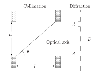
Figure 2: Collimation setup and diffraction grating. For clarity the diagram is not in scale.

An evaluation of the initial coherence length $\ell_{0}$ for fullerene experiments is reported in Tab. 3.

V The Interference pattern

Consider now the initial density matrix $\rho_{0}$ given by Eq. (36). Define

$$\frac{1}{2\ell(t)^{2}}\>\equiv\>\frac{\Lambda\,t}{3}\,+\,\frac{1}{2\ell_{0}^{2}}\,,\quad\mbox{i.e.,}\quad\ell(t)\,\equiv\,\frac{\ell_{0}}{\sqrt{1+\frac{2\Lambda\,t}{3}\,\ell_{0}^{2}}}\,$$ (39)

(note that $\ell(0)=\ell_{0}$). Then Eq. (29) becomes

$$\rho(x,x^{\prime},t)=\frac{M}{2\pi\hbar t}\!\iint\!\!\mathrm{d}x_{0}\,\mathrm{d}x_{0}^{\prime}\>\exp\bigg{\{}\>\frac{iM}{2\hbar t}\bigg{[}(x-x_{0})^{2}-(x^{\prime}-x_{0}^{\prime})^{2}\bigg{]}-\>\frac{(x_{0}-x_{0}^{\prime})^{2}}{2\ell(t)^{2}}-\frac{\Lambda\,t}{3}\bigg{[}(x-x^{\prime})^{2}+(x-x^{\prime})(x_{0}-x_{0}^{\prime})\bigg{]}\!\bigg{\}}\widetilde{\rho}_{0}(x_{0},x_{0}^{\prime}),$$

whence, from relation (17), the intensity on the screen is given by

$$I_{2}(x)\ \equiv\ \rho(x,x,T)\ =\ \frac{M}{2\pi\hbar T}\!\iint\!\!\mathrm{d}x_{0}\,\mathrm{d}x_{0}^{\prime}\exp\bigg{\{}\frac{iM}{2\hbar T}\bigg{[}x_{0}^{2}-x_{0}^{\prime 2}+2x(x_{0}^{\prime}-x_{0})\bigg{]}-\frac{(x_{0}-x_{0}^{\prime})^{2}}{2\ell^{2}}\bigg{\}}\,\widetilde{\rho}_{0}(x_{0},x_{0}^{\prime}),$$ (40)

where $x_{0}$ and $x_{0}^{\prime}$ run along the slits crossed by the initial wave function whose support is $\Delta x$ and $\ell\equiv\ell(T)$ is the coherence length at the time of flight $t=T$.

As already argued for $\ell_{0}$, if $\ell\lesssim\Delta x$ the exponential $\smash{\exp[-(x_{0}-x_{0}^{\prime})^{2}/(2\ell^{2})]}$ reduces from $\Delta x$ to $\ell$ the length scale on which the initial state is coherent. This scale is fixed from both geometry of the experimental setup, i.e., the collimation apparatus and the distance $L$ between grating and screen, and the physical conditions under which the interferometry takes place, i.e., the momentum of the macromolecule and the effect of the environment (see Eqs. (39) and (8)). On the other hand, the above exponential does not give any relevant contribution if $\ell~{}\gg~{}\Delta x$, and, from Eqs. (38) and (39), it follows that this occurs when there are both good collimation ($\theta\approx 0$) and negligible coupling with surrounding environment ($\Lambda\approx 0$). In this case we fall back to the treatment of section II.1.

Note that interference fringes appear on the detection screen if $\Delta x\gtrsim D$ and $\ell\gtrsim D$, i.e., if the molecules are coherent at least on two contiguous slits. The numerical estimates of $\ell_{0}$ and $\ell$ in the condition of fullerene experiments are shown in Tab. 3. In particular, note that $\ell\approx D$ and thus interference is mainly due to adjacent slits. Moreover, a comparison between the values of $\ell_{0}$ and $\ell$ shows that the main mechanism which yields a loss of coherence is the angular divergence of the beam .

Table 3: Comparison between losses of coherence in fullerene experiments arnzei99 ; JMO2000 .

Initial coherence length ($t=0$):	$\ell_{0}\,\approx\,1.3\times 10^{-7}\,\mathrm{m}$
Coherence length at $t=T$:	$\ell\,\sim\,D\,=10^{-7}\,\mathrm{m}$

V.1 Fraunhofer approximation for the intensity

We shall now proceed to an approximate evaluation of $I(x)$, relying on conditions that are reasonable in common interferometry experiments performed in far-field approximation (see App. A for a more refined evaluation in the case of a pair of Gaussian shaped slits).

Note that

$$\exp\bigg{[}\frac{iM(x_{0}^{2}-x_{0}^{\prime 2})}{2\hbar T}\bigg{]}\approx 1$$

when

$$\frac{M(x_{0}^{2}-x_{0}^{\prime 2})}{2\hbar T}=\frac{M(x_{0}+x_{0}^{\prime})(x_{0}-x_{0}^{\prime})}{2\hbar T}\ll 1$$

and this condition is clearly satisfied in the Fraunhofer regime (13). Nevertheless, in the presence of a coherence length $\ell\lesssim\Delta x$, we have relevant contributions in integration (40) just for $(x_{0}-x_{0}^{\prime})\lesssim\ell$. Thus, under the condition

$$\frac{M\Delta x\,\ell}{\hbar T}\ll 1\,,$$ (41)

$I_{2}(x)$ gets approximated by

$$I_{3}(x)=\frac{M}{2\pi\hbar T}\!\iint\!\!\mathrm{d}x_{0}\,\mathrm{d}x_{0}^{\prime}\exp\bigg{[}\frac{iMx}{\hbar T}(x_{0}^{\prime}-x_{0})\bigg{]}\,{\rho}_{1}(x_{0},x_{0}^{\prime}),$$ (42)

where

$${\rho}_{1}(x_{0},x_{0}^{\prime})=\exp\bigg{[}-\frac{(x_{0}-x_{0}^{\prime})^{2}}{2\ell^{2}}\bigg{]}\,\widetilde{\rho}_{0}(x_{0},x_{0}^{\prime})\,.$$

Introducing the Fourier transform of $\rho_{1}$

$$\widehat{\rho}_{1}(k_{0},k_{0}^{\prime})=(2\pi)^{-1}\!\iint\!\mathrm{d}x_{0}\mathrm{d}x_{0}^{\prime}\,e^{-i(k_{0}\,x_{0}+k_{0}^{\prime}\,x_{0}^{\prime})}\>\rho_{1}(x_{0},x_{0}^{\prime})\,$$

we have

$$I_{3}(x)=\frac{M}{\hbar T}\,\widehat{\rho}_{1}(\bar{k},-\bar{k}),\quad\mbox{where}\quad\bar{k}\equiv\frac{Mx}{\hbar T}=\frac{2\pi x}{\lambda L}.$$ (43)

This result is very analogous to Eq. (11) of section II.1 with (41) replacing (10) whenever $\ell\lesssim\Delta x$. Also in this case (41) should be rewritten in terms of the physical variables under control (cf. (12)), namely as

$$\frac{\ell}{L}\ll\frac{\lambda}{\Delta x}\,.$$

This notwithstanding, there are some basic difference that should be underlined: First, $\rho_{1}$ is not the initial state, but it is an effective state that takes into account incoherence due to preparation and to the time evolution. In fact $\ell$ depends on the physical and geometrical variables of the experiment in the phase of preparation and in its future development and it is progressively reduced by increasing the time of flight. Second, unlike what typically happens in the framework of classical optics and the theory of scattering, it is no more useful to evaluate $\rho_{1}$ asymptotically in time, since environmental-induced decoherence completely destroys interference fringes at times too large.

In fullerene experiments, $\ell\approx 10^{-7}$ m $<\Delta x\approx 10^{-6}\,\mathrm{m}$ (for an estimate of $\Delta x$, see Section VII). In this case the left-hand side (LHS) of (41) is not at all negligible with respect to unity. Anyhow, a more precise inspection of integration (40), with $\widetilde{\rho}_{0}$ given by (34), shows that condition (41) is a too strong demand and that approximation (42) can be reasonably applied. So doing, the error made is not completely negligible only for the pair of adjacent slits farthest with respect to the optical axis. This error, however, affects negligibly the sum involving the contributions of all the slits.

Let us now compute $\widehat{\rho}_{1}(\bar{k},-\bar{k})$ for $\widetilde{\rho}_{0}$ expressed by (34), i.e., for the split of macromolecules on a periodic grating of period $D$. First we make the change of variables $\xi\equiv x_{0}+sD/2$ and $\xi^{\prime}\equiv x_{0}^{\prime}+s^{\prime}D/2$, which leads to

$$\widehat{\rho}_{1}(\bar{k},-\bar{k})=\frac{1}{2\pi}\sum_{s,s^{\prime}}e^{\,i\bar{k}(s-s^{\prime})\frac{D}{2}}\,e^{-\frac{[(s-s^{\prime})D/2]^{2}}{2\ell^{2}}}\iint\mathrm{d}\xi\mathrm{d}\xi^{\prime}\,e^{-i\bar{k}\xi}\,e^{i\bar{k}\xi^{\prime}}\,e^{\frac{1}{2\ell^{2}}\big{[}(\xi^{\prime}-\xi)(s^{\prime}-s)D-(\xi^{\prime}-\xi)^{2}\big{]}}\,\varphi(\xi)\;\varphi(\xi^{\prime})^{*}\,,$$ (44)

and second we perform the Taylor series expansion of the real exponential in the previous integral in the variable $(\xi^{\prime}-\xi)/\ell$ and about the point $\xi^{\prime}=\xi$

$$\exp\bigg{[}\frac{(\xi^{\prime}-\xi)(s^{\prime}-s)D-(\xi^{\prime}-\xi)^{2}}{2\ell^{2}}\bigg{]}=1+\frac{(\xi^{\prime}-\xi)(s^{\prime}-s)D}{2\ell^{2}}+O\bigg{[}\bigg{(}\frac{\xi^{\prime}-\xi}{\ell}\bigg{)}^{2}\bigg{]}.$$ (45)

The solution of Eq. (44) is particularly handy whenever the effects due to incoherence are negligible on a length scale of the order of the slit width $d$ or, in other words, whenever the strength of incoherence does not spatially resolve the single slit. This is assured by a slit width much less than the coherence length

$$d/\ell\ll 1.$$ (46)

Under condition (46) the LHS of Eq. (45) is well approximated by $1$. In fact, since $\xi$ and $\xi^{\prime}$ run within the slit width $d$ and $(s^{\prime}-s)D/2\lesssim\ell$ due to the damping exponential $\exp\Big{\{}\!\!-\![(s-s^{\prime})D/2]^{2}/(2\ell^{2})\Big{\}}$ in Eq. (44), we have

$$\frac{(\xi^{\prime}-\xi)(s^{\prime}-s)D}{2\ell^{2}}\ \lesssim\ d/\ell\ll 1.$$

Thus the Fourier transform (44) becomes

$$\widehat{\rho}_{1}(\bar{k},-\bar{k})\>\sim\>\frac{1}{2\pi}\sum_{s,s^{\prime}}e^{\,i\bar{k}(s-s^{\prime})\frac{D}{2}}\,e^{-\frac{[(s-s^{\prime})D/2]^{2}}{2\ell^{2}}}\iint\mathrm{d}\xi\mathrm{d}\xi^{\prime}\,e^{i\bar{k}\xi}\,e^{-i\bar{k}\xi}\varphi(\xi)\;\varphi(\xi^{\prime})^{*}.$$

(Although the rough condition (46) is not directly satisfied in fullerene experiments, the zero-order approximation of (45) can be reasonably applied in integration (44); for an evaluation of the error introduced the reader can see App. B).

In the light of these considerations, the intensity pattern is well approximated by

$$I_{4}(x)\>=\>\frac{M}{\hbar T}\big{|}\widehat{\varphi}(\bar{k})\big{|}^{2}\sum_{s,s^{\prime}}e^{\,\frac{i\bar{k}}{2}(s-s^{\prime})D}\,e^{-\frac{[(s^{\prime}-s)D/2]^{2}}{2\ell^{2}}}\,,$$

where $\widehat{\varphi}$ is the Fourier transform of $\varphi$.

Note that the sum of the terms with $s=s^{\prime}$ simply gives $N$, while the sum of the terms with $s\neq s^{\prime}$ gives

$$2\sum_{s>s^{\prime}}e^{-\frac{[(s^{\prime}-s)D/2]^{2}}{2\ell^{2}}}\!\cos\bigg{[}\frac{\bar{k}(s^{\prime}-s)}{2}\bigg{]}.$$

By adding these two contributions and with $\bar{k}=~{}2\pi x/(\lambda L)$ (see Eq. (43)), we arrive at the suggestive “Fraunhofer-like” expression

$$I_{4}(x)\>\equiv\>I(x)\>=\>\frac{2\pi}{\lambda L}\,\bigg{|}\,\widehat{\varphi}\bigg{(}\frac{2\pi x}{\lambda L}\bigg{)}\bigg{|}^{2}\,\bigg{[}N+2\sum_{n=1}^{N-1}(N-n)\,e^{-\frac{(nD)^{2}}{2\ell^{2}}}\!\cos\bigg{(}\frac{2\pi nDx}{\lambda L}\bigg{)}\bigg{]}$$ (47)

(being understood that for $N=1$ the sum is zero), where $n=(s^{\prime}-s)/2$ .

Equation (47) shows that, whereas all the $N$ wave packets outgoing from the grating contribute to the intensity revealed on the screen, the pairs of slits which concretely contribute to interference oscillations are distant at most of the order of $\ell$, due to the damping exponential in the sum. It follows that, for a finite $\ell$, the interference pattern shows “distortions” in fringe structure due to partially random preparation and decoherence, but, being incoherent effects typically negligible on single-slit space scale, fringe pattern is just modulated by the single-slit diffraction profile, $|\widehat{\varphi}|^{2}$, according to classical optics Fraunhofer diffraction.

As already sketched before, it should be observed that the intensity on the screen may show interference fringes only if the coherence length is at least as long as the grating period, i.e.,

$$\ell(t)\gtrsim D$$ (48)

(note that this inequality should be satisfied at least at the initial time $t=0$). For positive times, recalling (39), we obtain

$$t\lesssim\tau_{c}\equiv\frac{3}{2\Lambda D^{2}}\bigg{[}1-\bigg{(}\frac{D}{\ell_{0}}\bigg{)}^{2}\bigg{]},$$

which provides an upper bound for the time of flight, i.e., an evaluation for the effective coherence time $\tau_{c}$. Note that for the fullerene experiment, according to Tab. 1 and Tab. 2, it results

$$\tau_{c}=4\times 10^{-2}\mbox{s}\,,$$

which is indeed several times the value of the time of flight in this experiment .

The effective coherence time $\tau_{c}$ is clearly an upper bound for the time of flight $T$, since interference fringes are detectable only within $\tau_{c}$. This shows that the “geometrical optics” limit in presence of decoherence requires more care than in the free case. In particular, it can not be based on the standard time-independent methods and the “$t\to\infty$” limit.

V.2 Extension to a generic angular divergence of the beam

This section is devoted to generalize Eq. (47) for a generic transversal wave number probability distribution $p\,(k_{x})$. Introducing Eqs. (30) and (33) in Eq. (29), the long-time asymptotic behavior of the intensity becomes

$$I_{3}(x)\>=\>\frac{M}{\sqrt{2\pi}\hbar T}\!\iint\!\!\mathrm{d}x_{0}\,\mathrm{d}x_{0}^{\prime}e^{i\bar{k}\,(x_{0}^{\prime}-x_{0})-\frac{\Lambda T}{3}\,(x_{0}^{\prime}-x_{0})^{2}}\,\widehat{p}\,(x_{0}^{\prime}-x_{0})\,\widetilde{\rho}_{0}(x_{0},x_{0}^{\prime}).$$

By the same variable change which leads to Eq. (44) and making explicit $\widetilde{\rho}_{0}$ for a grating of period $D$ (cf. Eq. (34)), we obtain

$$\begin{split}I_{3}(x)\>=\>&\frac{M}{\sqrt{2\pi}\hbar T}\sum_{s,s^{\prime}}e^{\,i\bar{k}(s-s^{\prime})\frac{D}{2}}\,e^{-\frac{\Lambda T}{3}[(s^{\prime}-s)D/2]^{2}}\\ &\times\iint\mathrm{d}\xi\mathrm{d}\,\xi^{\prime}\,e^{\,-i\bar{k}\xi}\,e^{\,i\bar{k}\xi^{\prime}}\,e^{-\frac{\Lambda T}{3}\big{[}(\xi^{\prime}-\xi)^{2}+(\xi^{\prime}-\xi)(s^{\prime}-s)D\big{]}}\,\widehat{p}\,\big{[}\xi^{\prime}-\xi+(s-s^{\prime})D/2\big{]}\,\varphi(\xi)\;\varphi(\xi^{\prime})^{*}.\end{split}$$ (49)

As discussed in the preceding section, note that $|\xi^{\prime}-\xi|\leq d$ and that $|(s^{\prime}-s)D/2|_{\rm max}\sim(\Lambda T)^{-1/2}$ due to the damping term $e^{-\frac{\Lambda T}{3}[(s^{\prime}-s)D/2]^{2}}$ in Eq. (49). Thus, in case of decoherence negligible on the single-slit length scale, i.e., for $d(\Lambda T)^{1/2}\ll 1$, and for a slowly varying function $\widehat{p}$, such that $\widehat{p}\,\big{[}\pm d+(s-s^{\prime})D/2\big{]}\sim\widehat{p}\,\big{[}(s^{\prime}-s)D/2\big{]}\ \forall\,s,s^{\prime}$, Eq. (49) becomes

$$I(x)\>=\>\frac{(2\pi)^{3/2}}{\lambda L}\,\widehat{p}\,(0)\,\bigg{|}\,\widehat{\varphi}\bigg{(}\frac{2\pi x}{\lambda L}\bigg{)}\bigg{|}^{2}\,\bigg{\{}N+2\sum_{n=1}^{N-1}(N-n)\,e^{-\frac{\Lambda T}{3}(nD)^{2}}\,\bigg{[}\frac{\widehat{p}\,(nD)}{\widehat{p}\,(0)}\bigg{]}\,\cos\bigg{(}n\frac{2\pi Dx}{\lambda L}\bigg{)}\bigg{\}},$$ (50)

where $n=(s^{\prime}-s)/2$ and $\bar{k}=2\pi x/(\lambda L)$. Note that the assumption of slow variation of $\widehat{p}$ is directly assured by a sufficient sharpness of the wave number distribution $p\,(k_{x})$, i.e., by $\Delta k_{x}\ll d^{-1}$.

VI Quantum interferometry and classical diffraction theory

VI.1 Comparison with geometrical optics

In case of complete coherence, i.e., for $p\,(k_{x})=\delta(k_{x})$ and $\Lambda=0$, Eq. (50) reduces to the well-known Fraunhofer relation for optical diffractive patterns

$$\begin{split}I(x)&\>=\>\frac{2\pi}{\lambda L}\,\bigg{|}\widehat{\varphi}\bigg{(}\frac{2\pi x}{\lambda L}\bigg{)}\,\sum_{n=0}^{N-1}e^{\,in\frac{2\pi Dx}{\lambda L}}\bigg{|}^{2}\\ &\ =\ \frac{2\pi}{\lambda L}\,\bigg{|}\widehat{\varphi}\bigg{(}\frac{2\pi x}{\lambda L}\bigg{)}\bigg{|}^{2}\,\bigg{[}\frac{\sin(\pi NDx/\lambda L)}{\sin(\pi Dx/\lambda L)}\bigg{]}^{2}.\end{split}$$

Moreover, for just two slits ($N=2$), i.e., for Young double-slit interference, Eq. (50) becomes

$$\begin{split}I(x)\>=\>&\frac{4\pi}{\lambda L}\,\widehat{p}\,(0)\,\bigg{|}\widehat{\varphi}\bigg{(}\frac{2\pi x}{\lambda L}\bigg{)}\bigg{|}^{2}\\ &\times\bigg{[}1+\frac{\widehat{p}\,(nD)}{\widehat{p}\,(0)}\,e^{-\frac{\Lambda M\lambda L}{6\pi\hbar}D^{2}}\!\cos\bigg{(}\frac{2\pi Dx}{\lambda L}\bigg{)}\bigg{]}.\end{split}$$

This expression is very similar to that used in classical optics to describe interference patterns due to partially coherent electromagnetic fields wolf . In particular, note that the damping term for quantum interference oscillations

$$\mathcal{V_{\mathrm{QM}}}\ =\ \frac{\widehat{p}\,(nD)}{\widehat{p}\,(0)}\,e^{-\frac{\Lambda M\lambda L}{6\pi\hbar}D^{2}}$$ (51)

is the quantum-mechanical counterpart of the fringe visibility $\mathcal{V_{\mathrm{CO}}}$ of classical optics

$$\mathcal{V_{\mathrm{QM}}}\ \longleftrightarrow\ \mathcal{V_{\mathrm{CO}}}.$$ (52)

Both for quantum and classical interferometry, the visibility $\mathcal{V}$ is a measure of the distinctness of the fringes and is defined by

$$\mathcal{V}\ =\ \frac{I_{\rm max}-I_{\rm min}}{I_{\rm max}+I_{\rm min}}\,.$$ (53)

The intensities $I_{\rm max}$ and $I_{\rm min}$ are, respectively, the maximum and the minimum revealed on the detection screen in the immediate neighborhood of the optical axis.

Now it is useful to recall an important result from the classical theory of partial coherence. The pattern visibility $\mathcal{V_{\mathrm{CO}}}$ of a quasimonochromatic field, equally split by a pair of slits, coincides with the modulus of the spectral degree of coherence $\mu(\lambda)$ wolf ; otto , which characterizes the field correlation in the space-frequency domain

$$\mathcal{V_{\mathrm{CO}}}\ =\ |\mu(\lambda)|.$$ (54)

From Eqs. (53) and (54) it follows that the degree of spectral coherence is upper bounded by unit, value assumed in condition of complete coherence (e.g., in case of laser radiation diffraction).

According to the correspondence (52), the results of the classical theory of partial coherence extends to quantum systems, mutata mutandis. For instance, in Section VIII we shall show some interesting analogies concerning with temporal and spatial coherence of beams, while in the following we underline the differences existing between classical optics and quantum mechanics.

First of all, the degree of coherence of quantum particles depends both on the collimation of the macromolecular beam and on the strength of interaction with the surrounding environment during the time of flight (cf. Eq. (51)). In optics, instead, the degree of coherence of quasimonochromatic fields is only due to source details. More particularly, the corruption of visibility of interfering fields increases with the spatial extension of the source, composed by a statistical ensemble of many independent elementary radiators.

Moreover, in classical optics the explicit form of the degree of coherence $\mu(\lambda)$ depends on the geometrical shape of the source, while the damping term $\mathcal{V}_{\mathrm{QM}}$ depends both on the features of the evolution kernel (30), characterizing the decoherence model, and on the geometrical details of the collimation apparatus (cf. Eq. (51)).

VI.2 Fresnel regime and Talbot interferometry

We would like now to comment on interferometry in the near-field zone klauser ; chapman ; nowak ; kimble , which has been recently realized by means of $C_{70}$ beams ztalbot ; ztalbot2 . Such experiments show that, at distances from the diffraction grating multiple of the length $2D^{2}/\lambda$, images of the grating itself are reconstructed (see also the optical Talbot effect talbot ; winthrop ).

Thus, by shifting another identical grating, placed behind the previous one at a distance $2D^{2}/\lambda$, the integrated signal outgoing from the gratings periodically changes from its minimum (half period displacement of the two gratings) to its maximum (complete alignment).

If the influence of the environment is negligible, a treatment of this effect in the spirit of Section  II.1 can be performed. In fact, given the correspondence between Helmholtz and stationary Schrödinger equation, one can directly exploit the standard optical techniques, such as Fresnel-Kirchhoff diffraction integrals in Fresnel zone, with suitable boundary conditions—“transmission functions”—at the gratings. Indeed, this is what it has been done (see, e.g., kimble ; ztalbot3 ) by means of the so-called “paraxial approximation,” assuming both gratings distances large with respect to the grating period and an infinite number of slits.

In experiments with large molecules ztalbot2 , it has been observed that the visibility of the signal is progressively reduced by increasing the pressure of environmental gas, a clear sign of environmental quantum decoherence. A quantitative explanation of this effect—using the model of Joos and Zeh in order to suitably modify the classical Fresnel-Kirchhoff description recalled above—has been already provided in ztalbot2 . A more self-contained and thorough analysis, based on Eq. (17), will be presented elsewhere fut . Here we shall provide just a sketchy outline, referring to a theoretical treatment already present in literature schleich . In this last work, the form of the propagator describing the free evolution of a quantum wave is shown, split by a diffraction grating with a formally infinite number of slits, i.e., with an associated initial density matrix of the form

$$\rho_{0}(x,x^{\prime})\,=\!\sum_{j,j^{\prime}\in\mathbb{Z}}\!\varphi(x+jD)\;\varphi(x^{\prime}+j^{\prime}D)^{*}$$ (55)

(note that, with respect to initial state expressed by (33) and (34), here it is assumed perfect collimation and an infinite number of slits). Let $\smash{K^{\text{\scriptsize(free)}}_{T}}$ be the so called Talbot propagator, including the sum over $j$ and $j^{\prime}$ of (55) and, accordingly, providing the intensity pattern $I(x)$ in term of the single wave packet $\varphi(x)$:

$$I(x)\propto\int\mathrm{d}x_{0}\,\mathrm{d}x_{0}^{\prime}\>K^{\text{\scriptsize(free)}}_{T}(x,x,t;x_{0},x_{0}^{\prime},0)\,\varphi(x_{0})\;\varphi(x_{0}^{\prime})^{*}\,.$$ (56)

It results (see e.g. schleich ) that, at a distance $L_{T}$ from the grating equal to $2D^{2}/\lambda$, or multiple of it (and consequently at times $t_{T}$ multiples of $L_{T}/v=2MD^{2}/h$), $\smash{K^{\text{\scriptsize(free)}}_{T}}$ reduces to

$$\begin{array}[]{ll}\displaystyle K^{\text{\scriptsize(free)}}_{T}(x,x,t_{T};x_{0},x_{0}^{\prime},0)&\displaystyle=\frac{1}{D^{2}}\sum_{j=-\infty}^{+\infty}\exp\bigg{(}-2\pi ij\frac{x-x_{0}}{D}\bigg{)}\sum_{j^{\prime}=-\infty}^{+\infty}\exp\bigg{(}-2\pi ij^{\prime}\frac{x-x^{\prime}_{0}}{D}\bigg{)}\\ &\displaystyle=\sum_{j=-\infty}^{+\infty}\delta(x-x_{0}+jD)\,\sum_{j^{\prime}=-\infty}^{+\infty}\delta(x-x^{\prime}_{0}+j^{\prime}D).\end{array}$$ (57)

Clearly, from this relation and Eq. (56) it is immediate to verify that the final state is an exact reconstruction of the initial one (55).

By following the same steps leading to Eq. (57), but now using the propagator (30) which embodies the incoherence effects, the Talbot propagator becomes

$$\begin{array}[]{ll}\displaystyle K^{\text{\scriptsize(env)}}_{T}(x,x,t_{T};x_{0},x_{0}^{\prime},0)=&\displaystyle\frac{1}{D^{2}}\sum_{j=-\infty}^{+\infty}\exp\bigg{(}-2\pi ij\frac{x-x_{0}}{D}\bigg{)}\>\exp\bigg{\{}-2j^{2}\bigg{[}\frac{D}{\ell(t_{T})}\bigg{]}^{2}\bigg{\}}\\ &\ \times\displaystyle\sum_{j^{\prime}=-\infty}^{+\infty}\exp\bigg{(}-2\pi ij^{\prime}\frac{x-x^{\prime}_{0}}{D}\bigg{)}\>\exp\bigg{\{}-(2{j^{\prime}}^{2}+4jj^{\prime})\bigg{[}\frac{D}{\ell(t_{T})}\bigg{]}^{2}\bigg{\}}\,,\end{array}$$

where $\ell(t_{T})$ is the coherence length computed at the Talbot time $t_{T}$. With respect to Eq. (57), here some additional exponential are present which obstructs the reconstruction of the initial wave function. So, if we put a second grating at distances multiples of $2D^{2}/\lambda$, even for a perfect alignment between the two gratings the wave function is partially stopped and thus the intensity detected will be lower than in the free case. Similarly, for a displacement between the gratings of an half period, a portion of signal, even little, may be detectable further on. In such a scenario, a decrease of the coherence length $\ell$, i.e., a growth of the incoherence of the beam, leads to a progressive reduction of the visibility of the total intensity on the screen, in agreement with the behaviour of the experimental data reported in ztalbot2 . (An improvement of this analysis should presumably take into account: 1) the three free-standing gratings for the Talbot-Lau interferometer effectively used in experiments; 2) a proper description of the van der Waals interaction with the grating).

VI.3 Near-field interferometry and randomness of arrival times

Near-field interferometry, such as Talbot-Lau interferometry, should allow us to probe quantum effects also due to the motion along the longitudinal direction, which so far has been treated as classical. Such a treatment has been of course completely motivated by the experimental conditions considered so far for which both (5) and (7) are satisfied with a high degree of approximation. But suppose that position spread in the longitudinal direction $\Delta y$ is not completely negligible with respect to $L$. Then the arrival times would have statistical fluctuations of order

$$\Delta T\sim\Delta y/v.$$

For the fullerene experiments in the Fraunhofer region such fluctuations are not appreciable: in this case, $\Delta T\sim~{}\Delta y/v\approx 5\times 10^{-9}\,\mathrm{s}$, and since $T\approx 6\times 10^{-3}\,$s, we have

$$\Delta T\ll T.$$ (58)

Near-field interferometry, possibly with light particles, should be able to test the measured intensity when (58) is violated. A first prediction is immediately suggested by (6): the measured intensity is obtained by the intensity distribution consider so far, namely $\rho(x,x,T)$, by convolution with $|\phi_{0}|^{2}$. Thus, randomness of the arrival times appears as an independent noise on the standard interference profile, which reduces the fringe visibility as it were an additional source of “decoherence”. This effect could be confused with a sort of intrinsic decoherence (in this regard see a recent proposal concerning atomic diffraction by standing light wave bonifacio ).

More generally, one may analyze the predictions of (3) in the mesoscopic regime nino . Let us consider a monochromatic beam, devoid of angular divergence, composed by free light particles of mass $m$. Let the beam be diffracted by two slits of width $d$ and distance $D$. It is convenient to describe the split wave function $\Psi({\bf r})$ by means of two-bidimensional Gaussian wave packets, whose barycenters move parallel to the optical axis $y$ with the velocity $v=\hbar k_{y}/m$:

$$\begin{split}\Psi({\bf r})&=\psi_{0}(x)\phi_{0}(y)\\ &=C\bigg{[}\sum_{s=\pm}e^{-\frac{(x-sD/2)^{2}}{4\sigma_{x}^{2}}}\bigg{]}\,e^{-\frac{y^{2}}{4\sigma_{y}^{2}}\,+\,ik_{y}y}.\end{split}$$ (59)

The constant $C$ ensures normalization. The transversal standard deviation $\sigma_{x}$ of each wave packet is related to the slit width $d$ (a typical assumption is $6\sigma_{x}=d$), while the longitudinal one is related to the extension of the initial support of $\Psi({\bf r})$.

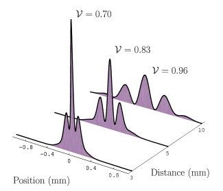
Figure 3: Double-slit interference patterns for different values of the distance between the grating and the detection screen. Patterns are obtained for ultra-cold neutrons ($v\approx 1\,\mathrm{m/s}$) diffracted by a pair of slits of width $d=5\times 10^{-6}\,\mathrm{m}$ and separated by a distance $D=10^{-5}\,\mathrm{m}$. Neutron initial wave function is described by means of bidimensional Gaussian wave packets with a longitudinal standard deviation $\sigma_{y}=10^{-3}\,\mathrm{m}$ and a transversal one $\sigma_{x}=d/6$.

After the splitting, we can consider that $\Psi({\bf r})$ evolves according to the free Schrödinger equation (2) until the particle is detected on the detection screen placed at a distance $L$. Given an arbitrary distance, not necessarily large compared with the size of the support of $\Psi({\bf r})$, and for a free evolution, the intensity detected at $y=L$ can be calculated by means of Eq. (4), with $\psi(x,t)$ and $\phi(x,t)$ obtained by the free evolution of the initial state (59). The result of such a numerical simulation for ultra-cold neutrons is shown in Fig. 3. At distances as short as to be comparable with the longitudinal spread of neutron wave packets, the statistical fluctuations on arrival times produce an appreciable reduction of the fringe visibility just as it would happen in case of an incoherent preparation of the beam and/or in case of environmental-induced decoherence. The only difference consisting in the distance dependence of the different processes: this kind of “decoherence” reduces by increasing the distance, environmental-induced decoherence increases, while the effects due to incoherent preparation are independent.

In particular, notice that the reduced visibility is not due, not even partially, to an incomplete wave-packet superposition, being this ensured, also for the shortest distance shown in Fig. 3, by the large wavelength of ultra-cold neutrons. Thus, the loss of fringe contrast has to be ascribed only to arrival time fluctuations of the same order of the classical time of flight.

For simulations of Fig. 3 we used a longitudinal delocalization at the double-slit given by $\sigma_{y}=10^{-3}$ m. This assumption can be relaxed to shorter values still detecting results analogous to those shown by Fig. 3, but at shorter distances. In this case the spatial resolution required for efficient detection becomes higher. Conversely, for a larger longitudinal delocalization, intrinsic decoherence effects can be readily detected at larger distances by means of less refined detectors.

In conclusion, let us underline that, since very slow neutrons ($v\approx 1$  m/s) scheckenhofer characterized by a wide transversal support ($\Delta x\gtrsim 10^{-4}$ m) scheckenhofer ; gahler have been used in interferometry, we think that an experimental test of the predicted behavior shown in Fig. 3 might be indeed in the reach of present technology (not necessarily for the concrete situation we have simulated, which was mainly for illustrative purposes).

VII Numerical calculations

In this section we shall use Eq. (47) to fit the experimental data reported in JMO2000 . In this regard, note that Eq. (47) describes an ideal situation where an infinitely accurate detector measures the spatial intensity distribution of a strictly monochromatic beam. Some adjustments have to be carried out in order to include in our treatment the effects on the diffraction pattern due both to the velocity distribution characterizing the beam macromolecules and to the distortions unavoidably introduced during the measurement process zeil88 . Each of these corrections have to be implemented on the intensity level, since they consist in incoherent contributions.

The total intensity is obtained by the sum of the monochromatic components of the beam

$$\bar{I}(x)=\int\mathrm{d}\lambda\;f(\lambda)\,I(x,\lambda),$$ (60)

where $I(x,\lambda)$ is given by Eq. (47) and its dependence on $\lambda$ is shown by Eq. (8). The wavelength distribution $f(\lambda)\mathrm{d}\lambda$ is directly obtained by the supersonic velocity distribution $f(v)\mathrm{d}v$ characterizing the macromolecule ensemble JMO2000

$$f(v)\,\mathrm{d}v\,\propto\,v^{3}\exp\,\big{[}-(v-v_{0})^{2}/\hat{v}^{2}\big{]}\,{\rm d}v\,.$$ (61)

It describes beams in transition between effusive and slow jet sources scoles . The parameters $v_{0}$ and $\hat{v}$ depend both on the temperature of the beam and on the physical features of the given molecule and they are deduced by a best fit over experimental measurement of the velocity distribution (see Fig. 2 in JMO2000 ).

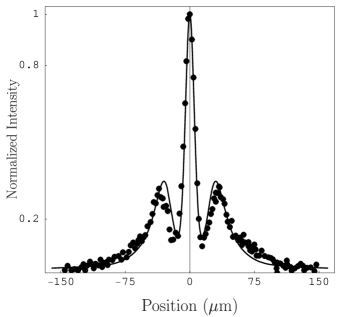
Figure 4: Theoretical fit and experimental data for $\mathrm{C}_{60}$ interferometry JMO2000 . Theoretical fit was performed considering $N=10$ equal, rectangular shaped, slits of an effective width $d=36\,\mathrm{nm}$. The spatial resolution of the detector is $2\widetilde{x}=8\,\mu{\rm m}$. The theoretical curve and experimental data are normalized to the value of the central maximum.

The finite spatial resolution can be taken into account by an integration over the size of the elementary detector, say $2\widetilde{x}$, weighed on its spatial response function $D(x)$. In particular, in the case of a flat response function, $D(x)$ becomes the characteristic function defined on the interval $\big{[}-\widetilde{x}\,,\,+\widetilde{x}\big{]}$ and the effective detected intensity is expressed by a moving average

$$I_{\mathrm{eff}}(x)\,=\,\int_{-\widetilde{x}}^{+\widetilde{x}}\mathrm{d}\zeta\>\bar{I}(x+\zeta)\>D(\zeta)\,=\,\frac{1}{2\widetilde{x}}\int_{x-\widetilde{x}}^{x+\widetilde{x}}\mathrm{d}\zeta\ \bar{I}(\zeta),$$

whence, from Eq. (60),

$$I_{\mathrm{eff}}(x)\ \,\propto\,\int_{x-\widetilde{x}}^{x+\widetilde{x}}\mathrm{d}\zeta\int\!\mathrm{d}\lambda\;f(\lambda)\,I(\zeta,\lambda).$$

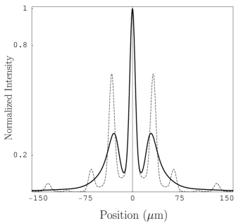
Figure 5: Interference patterns due both to a macromolecular beam characterized by a velocity distribution given by Eq. (61) as in JMO2000 (full line) and to a strictly monochromatic beam corresponding to the mean velocity (dashed line). The curves are normalized to the value of the central maximum.

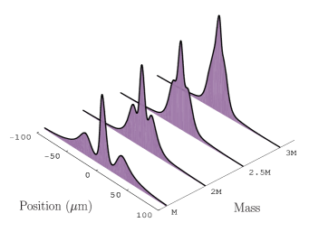
Figure 6: Diffraction of molecules with masses multiple of the $C_{60}$ mass $M$. For larger masses the quantum behavior becomes progressively negligible, approaching to the classical limit. Every curve has been normalized to the value of the central maximum obtained for the mass $M$.

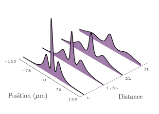
Figure 7: Interference patterns for different values of the distance between the grating and the detection screen, in unit of the value $L$ reported in JMO2000 . Increasing the distance the pattern spreads in position with respect to the optical axis. The visibility is reduced by the increased number of decohering events. Every curve has been normalized to the value of the central maximum obtained for the distance $L$.

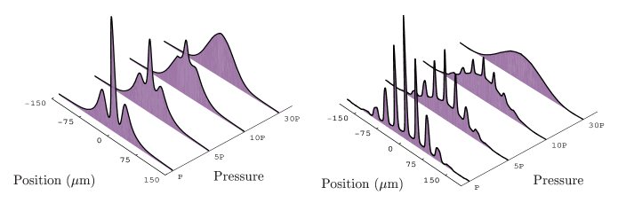
Figure 8: The two figures show interference patterns for increasing pressures at fixed temperature, in unit of the pressure $P=5\times 10^{-6}$Pa used in JMO2000 . Left figure corresponds to the experimental setup reported in JMO2000 : slit effective width $d=3.6\times 10^{-8}$ m and collimator aperture $a=10^{-5}$ m. Right figure has been obtained for narrower slits ($d=2\times 10^{-8}$ m), an improved collimation ($a=5\times 10^{-6}$ m) and a velocity selected $C_{60}$ beam ($\Delta v/v=10\%$, where $v$ is the mean velocity). Every curve has been normalized to the value of the central maximum at the pressure $P$.

For the free gap $d$ of the rectangular slits, it was used, according to grisenti , the effective width estimated in Refs. arnzei99 ; JMO2000 as previously discussed in Section IV . Moreover, a constant background has been subtracted from experimental data arnzei99 ; JMO2000 .

Finally, referring to Eq. (47), note that the number $N$ is basically a priori unknown, being the effective number of slits which concretely contribute to diffraction. In fact, only the knowledge of the fullerene wave function on the grating would allow us to fix the effective number of slits in which the initial wave function is split, since the width of collimation only gives information about the maximum number of wave packets which could contribute to the interference pattern. Nevertheless, $N$ can be easily inferred a posteriori as a free parameters of the fit with experimental data. So doing, we find $N=10$.

Our theoretical evaluation for the interference pattern is shown in Fig. 4, together with the experimental points published in Ref. JMO2000 , page 2819, Fig. 5.

VIII Conclusions and perspectives

One of the main goals of our work has been that of deducing, within the framework of Joos and Zeh model, a geometric optics limit of quantum mechanics in the presence of decoherence.

Our theoretical analysis confirms the negligibility of environmental disturbances in recent experiments of macromolecular interferometry arnzei99 ; JMO2000 with respect to the loss of coherence due to beam production.

Moreover, our analysis reproduces classical results, as well as Fraunhofer relation for optical diffractive patterns, and provides the quantum-mechanical analog for interferometry with partially coherent sources of radiation. For the latter subject, referring to the theory of partial coherence, existing analogies can be pointed out in a deeper way by exploiting numerical simulations. Fig. 5 clearly shows that, by selecting the particle beam velocity, the visibility of the corresponding interference pattern does not tend to unity, being upper bounded by the damping term $\mathcal{V}_{\mathrm{QM}}$ (cf. Eqs. (51)–(53)). On the other hand, the effect of the velocity selection makes more interference fringes visible at the border of the interference pattern.

The same behavior is obtained in the framework of classical optics, studying interference patterns due to quasimonochromatic fields wolf1 ; wolf2 . Classical partial coherence theory, supported by recent experiments otto2 , states that, by filtering, the pattern visibility at most approaches the value of the modulus of the degree of spectral coherence $\mu(\lambda)$, which depends on the spatial coherence of the source, and that more fringes becomes visible, since the temporal coherence is improved.

Moreover, our approach provides a useful theoretical framework for analyzing present (and possibly new) interference experiments. For instance, we have studied the mass dependence of the interference pattern due to the diffraction of heavy particles. Fig. 6 shows the simulations corresponding to beams of macromolecules heavier than $\mathrm{C}_{60}$, but characterized by the same physical features. Note that for larger masses the quantum behavior becomes progressively negligible, approaching to the classical limit. There are, indeed, other experimental investigations which support the previous expected behaviorarndt01 . They show that visibility of $\mathrm{C}_{70}$ diffracted beams is slightly reduced than that obtained for $\mathrm{C}_{60}$ ones in the same conditions.

In studying the effects of decoherence, it is particularly interesting to analyze the case of a diffracted quantum particle which experiences a lot of scattering events before reaching the detection screen. This situation is realized for larger grating-screen distances (see Fig. 7), or for more frequent scattering processes due, for example, to increasing value of pressure (see Fig. 8). In both cases the fringe visibility, and thus the wavelike behavior of the molecule, is progressively corrupted.

By improving the collimation of velocity selected $\mathrm{C}_{60}$ beams, the interference pattern shows a richer structure of fringes and thus a more evident quantum behavior. Moreover, interference oscillations appear also in less restrictive environmental conditions, provided that the signal-to-noise ratio is such to allow experimental detection. In fact, as shown by the right plot in Fig. 8, side maxima, far from the optical axis, which are not detected at pressure $P$ in experiments arnzei99 ; JMO2000 , turn out to be clearly visible even for pressures ten times larger than $P$. This might be relevant in devising new interferometry experiments directed to the study of the quantum behavior of macroscopic objects and also to test quantitatively the effects on a quantum subsystem due to external noise. Our suggestion has been partially realized in very recent experiments nairz03 , which show results in agreement with the prediction of Fig. 8.

Appendix A Young interference pattern with Gaussian slits

In the following we shall develop the exact solution of (40) in the case of slits with a Gaussian shaped profile. For simplicity we shall treat the case of interference patterns due to just a pair of slits of width $d$ and distance $D$, even though an analytical solution can be obtained also for a grating composed of several slits.

Let us consider an initial wave function split by two Gaussian slits of standard deviation $\sigma_{x}$ and centered at $x=\pm D/2$ (we can typically choose $6\sigma_{x}=d$)

$$\psi_{0}(x;k_{x})=\bigg{[}\varphi\Big{(}x+\frac{D}{2}\Big{)}+\varphi\Big{(}x-\frac{D}{2}\Big{)}\bigg{]}\,e^{i\,k_{x}\,x}=C\>\bigg{[}e^{-\frac{(x-D/2)^{2}}{4\sigma_{x}^{2}}}+e^{-\frac{(x+D/2)^{2}}{4\sigma_{x}^{2}}}\bigg{]}\,e^{i\,k_{x}\,x}\,,$$ (62)

where $C$ is the normalization constant. Inserting Eq. (32) in Eq. (40) with the initial state (62) we get

$$\begin{split}I(x)=\frac{MC^{2}}{2\pi\hbar T}\iint^{+\infty}_{-\infty}\!\!\!\!\!\!\!\!\!{\rm d}x_{0}\,{\rm d}x_{0}^{\prime}\,&\exp\bigg{\{}\frac{iM}{2\hbar T}\>\big{[}x_{0}^{2}-x_{0}^{\prime 2}+2x(x_{0}^{\prime}-x_{0})\big{]}-\frac{(x_{0}-x_{0}^{\prime})^{2}}{2\ell^{2}}\bigg{\}}\\ \times\sum_{s,s^{\prime}=\pm}&\exp\bigg{[}-\frac{\big{(}x_{0}+s\frac{D}{2}\big{)}^{2}}{4\sigma_{x}^{2}}-\frac{\big{(}x_{0}^{\prime}+s^{\prime}\frac{D}{2}\big{)}^{2}}{4\sigma_{x}^{2}}\bigg{]}\,,\end{split}$$

whence

$$I(x)\>=\>\frac{4M\sigma_{x}^{2}C^{2}}{\hbar T\sqrt{Q(T)}}\,\exp\bigg{[}-\frac{x^{2}+D^{2}/4}{Q(T)}\bigg{(}\frac{\sqrt{2}M\sigma_{x}}{\hbar T}\bigg{)}^{\!2}\,\bigg{]}\bigg{\{}\cosh\bigg{[}\bigg{(}\frac{\sqrt{2}M\sigma_{x}}{\hbar T}\bigg{)}^{2}\frac{Dx}{Q(T)}\bigg{]}+\exp\bigg{[}-\frac{D^{2}}{2Q(T)\ell^{2}}\bigg{]}\cos\bigg{[}\frac{MDx}{\hbar TQ(T)}\bigg{]}\bigg{\}},$$ (63)

where $Q(T)\equiv 1+\big{[}2M\sigma_{x}^{2}/(\hbar T)\big{]}^{2}+(2\sigma_{x}/\ell)^{2}$.

For $T\gg M\sigma_{x}D/\hbar$ and $\ell\gg\sigma_{x}$ the term $Q(T)\to 1$, the first exponential in Eq. (63) reduces to $\exp\big{\{}\!\!-~{}\!\!\![\sqrt{2}Mx\sigma_{x}/(\hbar T)]^{2}\big{\}}$, whence $x_{max}\approx\hbar T/(M\sigma_{x})$, and thus the argument of the hyperbolic cosine is close to zero. It follows that Eq. (63) is well approximated by (see Eq. (8))

$$I(x)\>=\>\frac{8\pi\sigma_{x}^{2}C^{2}}{\lambda L}\>\exp\bigg{[}\bigg{(}\frac{2\sqrt{2}\pi x\sigma_{x}}{\lambda L}\bigg{)}^{\!2}\,\bigg{]}\bigg{[}1+e^{-\frac{D^{2}}{2\ell^{2}}}\>\cos\bigg{(}\frac{2\pi Dx}{\lambda L}\bigg{)}\bigg{]}\>=\>\frac{4\pi}{\lambda L}\,\bigg{|}\widehat{\varphi}\bigg{(}\frac{2\pi x}{\lambda L}\bigg{)}\bigg{|}^{2}\,\bigg{[}1+e^{-\frac{D^{2}}{2\ell^{2}}}\>\cos\bigg{(}\frac{2\pi Dx}{\lambda L}\bigg{)}\bigg{]}\,,$$

which coincides with Eq. (47) evaluated for $N=2$.

Appendix B Approximation quality test for fullerene experiment

In this appendix we evaluate the error committed introducing the zero-order approximation of (45) in Eq. (44), referring to experimental conditions reported in JMO2000 .

Since $|(s^{\prime}-s)D|\lesssim 2\ell$, we will test the previous approximation in the most unfavorable situation, according to $\exp[(\xi^{\prime}-\xi)/\ell]\approx 1$. To this aim, it is useful to introduce the integrals

$$\mathcal{I}(\ell,\bar{k})=\int_{-\infty}^{+\infty}\!\!\!\!\!{\rm d}\xi\ \varphi(\xi)\,e^{\xi/\ell}\,e^{i\bar{k}\xi}\,,$$

$$A(\bar{k})=\int_{-\infty}^{+\infty}\!\!\!\!\!{\rm d}\xi\>\varphi(\xi)\,e^{i\bar{k}\xi}\,,$$

where $\bar{k}=Mx/(\hbar T)$. Zero-order approximation of (45) can be checked by evaluating the relative displacement of the square modulus of the previous integrals

$$R(\ell,\bar{k})=\bigg{|}\frac{|\mathcal{I}(\ell,\bar{k})|^{2}-|A(\bar{k})|^{2}}{|\mathcal{I}(\ell,\bar{k})|^{2}}\bigg{|}\,.$$

The less is the value assumed by $R(\ell,\bar{k})$, the better is the quality of the zero-order approximation of (45).

By making explicit $\varphi(\xi)$ with the characteristic function defined in the interval $[-d/2,d/2]$, a straightforward calculation leads to

$$\begin{split}|\mathcal{I}(\ell,\bar{k})|^{2}&\ =\ \frac{2}{1/\ell^{2}+\bar{k}^{2}}\,[\cosh(d/\ell)-\cos(\bar{k}d)],\\ |A(\bar{k})|^{2}&\ =\ d^{2}\,{\rm sinc}^{2}(\bar{k}d/2)\ =\ \frac{2}{\bar{k}^{2}}\,[1-\cos(\bar{k}d)],\end{split}$$

whence

$$R(\ell,\bar{k})=\bigg{|}1-\bigg{[}1+\frac{1}{(\ell\bar{k})^{2}}\bigg{]}\frac{1-\cos(\bar{k}d)}{\cosh(d/\ell)-\cos(\bar{k}d)}\bigg{|}\,.$$ (64)

In the limit of small $\bar{k}$ (i.e., for positions $x\approx 0$, close to the maximum of intensity), we get

$$\lim_{\bar{k}\to 0}R(\ell,\bar{k})=1-\frac{(d/\ell)^{2}}{2\,[\cosh(d/\ell)-1]}\sim\frac{(d/\ell)^{2}}{12}\approx 0.011\,.$$ (65)

This means that in correspondence of the greatest intensities the approximate expression just moves away from the correct one of about 1%.

Since $R(\ell,\bar{k})$ is an increasing function of $\bar{k}$, and thus of $|x|$, then the most unfavorable case takes place at the edge of the interference pattern, where, however, the intensity is negligible. By using $\bar{k}_{\rm max}\approx d^{-1}$ in evaluating (64), it results that $R(\ell,\bar{k}_{\rm max})$ does not significantly differ from evaluation (65).

References

- (1) M. Arndt, O. Nairz, J. Vos-Andræ, C. Keller, G. van der Zouw, and A. Zeilinger, Nature 401, 680 (1999).
- (2) O. Nairz, M. Arndt, and A. Zeilinger, J. Mod. Opt. 47, no. 14/15, 2811 (2000).
- (3) J. M. Combes, R. G. Newton, and R. Shtokhamer, Phys. Rev. D 11, 366 (1975).
- (4) M. Daumer, D. Dürr, S. Goldstein, and N. Zanghì, Lett. Math. Phys. 38, 103 (1996).
- (5) D. Dürr, S. Goldstein, S. Teufel, and N. Zanghì, Physica A 279, 416 (2000).
- (6) D. Dürr, K. Münch-Berndl, and S. Teufel, J. Math. Phys. 40, no. 4, 1901 (1999).
- (7) M. Daumer, D. Dürr, S. Goldstein, and N. Zanghì, J. Stat. Phys. 88, 967 (1997).
- (8) E. Joos and H. D. Zeh, Z. Phys. B 59, 223 (1985).
- (9) S. Goldstein, in Stanford Encyclopedia of Philosophy, edited by E. N. Zalta (Stanford University, Stanford, 2002), URL: http://plato.stanford.edu/archives/win2002/entries/qm-bohm/ .
- (10) C. R. Leavens, Phys. Lett. A 178, 27 (1993).
- (11) W. R. McKinnon and C. R. Leavens, Phys. Rev. A 51, 2748 (1995).
- (12) C. R. Leavens, Phys. Rev. A 58, 840 (1998).
- (13) G. Grübl and K. Rheinberger, J. Phys. A: Math. Gen. 35, 2907 (2002).
- (14) M. Born and E. Wolf, Principles of Optics, (Cambridge University Press, Cambridge, 1999).
- (15) V. Allori, D. Dürr, S. Goldstein, and N. Zanghì, J. Opt. B 4, 482 (2002).
- (16) D. Dürr, S. Goldstein, and N. Zanghì, J. Stat. Phys. 67, 843 (1992).
- (17) M. R. Gallis and G. N. Fleming, Phys. Rev. A 42, 38 (1990).
- (18) D. Giulini, E. Joos, C. Kiefer, J. Kupsch, I. O. Stamatescu, and H. D. Zeh, Decoherence and the Appearance of a Classical World in Quantum Theory, (Springer, Berlin, 1996).
- (19) D. Dürr, R. Figari, and A. Teta, J. Math. Phys. (to be published), e-print quant-ph/0210199.
- (20) A. Viale, Degree Thesis, Università degli studi di Genova, a.a. 2000/2001 (unpublished).
- (21) B. Vacchini, Phys. Rev. E 63, 066115 (2001).
- (22) B. Vacchini, J. Math. Phys. 42, 4291 (2001).
- (23) R. Alicki, Phys. Rev. A 65, 034104-1 (2002).
- (24) C. Brukner and A. Zeilinger, Philos. Trans. R. Soc. Lond. A 360, 1061 (2002).
- (25) M. R. Pederson and A. A. Quong, Phys. Rev. B 46, 13584 (1992).
- (26) W. Krätschmer, L. D. Lamb, K. Fostiropoulos, and D. R. Huffman, Nature 347, 354 (1990).
- (27) E. Kolodney, A. Budrevich, and B. Tsipinyuk, Phys. Rev. Lett. 74, 510 (1995).
- (28) B. Vacchini, A. Viale, M. Vicari, and N. Zanghì (in preparation).
- (29) R. E. Grisenti, W. Schöllkopf, J. P. Toennies, G. C. Hegerfeldt, and T. Köhler, Phys. Rev. Lett. 83, 1755 (1999).
- (30) K. Hornberger and J. E. Sipe, Phys. Rev. A 68, 012105 (2003).
- (31) L. Basano, P. Ottonello, G. Rottigni, and M. Vicari, Opt. Commun. 207, 77 (2002).
- (32) J. F. Clauser and S. Li, Phys. Rev. A 49, R2213 (1994).
- (33) M. S. Chapman, C. R. Ekstrom, T. D. Hammond, J. Schmiedmayer, B. E. Tannian, S. Wehinger, and D. E. Pritchard, Phys. Rev. A 51, R14 (1995).
- (34) S. Nowak, Ch. Kurtsiefer, C. David, and T. Pfau, Opt. Lett. 22, 1430 (1997).
- (35) O. Carnal, Q. A. Turchette, and H. J. Kimble, Phys. Rev. A 51, 3079 (1995).
- (36) B. Brezger, L. Hackermüller, S. Uttenthaler, J. Petschinka, M. Arndt, and A. Zeilinger, Phys. Rev. Lett. 88, 100404 (2002).
- (37) K. Hornberger, S. Uttenthaler, B. Brezger, L. Hackermüller, M. Arndt, and A. Zeilinger, Phys. Rev. Lett. 90, 160401 (2003).
- (38) H. F. Talbot, Philos. Mag. 9, 401 (1836).
- (39) J. T. Winthrop and C. R. Worthington, J. Opt. Soc. Am. 55, 373 (1965).
- (40) B. Brezger, M. Arndt, and A. Zeilinger, J. Opt. B 5, S82 (2003).
- (41) H. Mack, M. Bienert, F. Haug, F. S. Straub, M. Freyberger, and W. P. Schleich, in Experimental Quantum Comunication and Information, edited by F. De Martini and C. Monroe (Elsevier, Amsterdam, 2002).
- (42) S. Mancini and R. Bonifacio, J. Phys. B 34, 1909 (2001).
- (43) H. Scheckenhofer and A. Steyerl, Phys. Rev. Lett. 39, 1310 (1977).
- (44) R. Gähler and A. Zeilinger, Am. J. Phys. 59, 316 (1991).
- (45) A. Zeilinger, R. Gähler, C. G. Shull, W. Treimer, and W. Mampe, Rev. Mod. Phys. 60, no. 4, 1067 (1988).
- (46) Atomic and Molecular Beam Methods, edited by G. Scoles (Oxford Univ. Press, Oxford, 1988), Vol. 1.
- (47) E. Wolf, Opt. Lett. 8, 250 (1983).
- (48) E. Wolf and A. T. Friberg, Opt. Lett. 20, 623 (1994).
- (49) L. Basano, P. Ottonello, G. Rottigni, and M. Vicari, Appl. Opt. 42, 6239 (2003).
- (50) M. Arndt, O. Nairz, J. Petschinka, and A. Zeilinger, C. R. Acad. Sci. Paris, t.2, Série. IV, 581 (2001).
- (51) O. Nairz, M. Arndt, and A. Zeilinger, Am. J. Phys. 71, 319 (2003).