Discrete entanglement distribution with squeezed light

Abstract

We show how one can entangle distant atoms by using squeezed light. Entanglement is obtained in steady state, and can be increased by manipulating the atoms locally. We study the effects of imperfections, and show how to scale up the scheme to build a quantum network.

Distributing entanglement among different nodes in a quantum network is one of the most challenging and rewarding tasks in quantum information. This may allow to extend quantum cryptography over long distances by using quantum repeaters repeaters . Furthermore, it may lead to some practical applications in the context of secret sharing sharing or distributed quantum computation distributed . From the more fundamental point of view, it may allow to perform loophole free tests of Bell inequalities Bell .

In a quantum network photons are used to entangle atoms located at different nodes which store the quantum information. Local manipulation of the atoms using lasers allows then to process this information. In principle, one can construct quantum networks using discrete Cirac (qubit) or continuous variable entanglement PK (the one contained, for example, in two–mode squeezed states GardinerZoller ). However, the fact that Gaussian states cannot be distilled using Gaussian operations Gaussno may strongly limit the applications of continuous variable entanglement in quantum networks and repeaters.

There have been several proposals to obtain discrete entanglement of distant atoms using high-Q cavities. There are basically two kind of schemes Cirac ; Parkins1 ; Cabrillo ; Huelga : (1) [Fig. 1(a)] An atom A, driven by a laser, emits a photon into the cavity mode. The photon, after travelling through a fiber, enters the second cavity where it is absorbed by atom B, which is also driven by a laser Cirac ; Parkins1 . (2) [Fig. 1(b)] Both atoms are simultaneously driven by a laser in such a way that if a photon is detected at half way between the cavities, the atoms get projected into an entangled state Cabrillo ; Duan . Most of these schemes operate in a transitory regime; i.e., the entanglement is achieved at a specific time and the lasers have to be switched on and off appropriately. Moreover, dissipation may introduce imperfections in the desired entangled state. In this work we propose and analyze a scheme to distribute discrete entanglement which works in steady state. As opposed to these other schemes, dissipation is a necessary ingredient of our scheme which, as we will show, gives it a very robust character. Our scheme transforms continuous variable entanglement into discrete (qubit) entanglement and thus exhibits how this last kind of entanglement may still be very useful in the context of quantum networks. We show how a small amount of this kind of entanglement can be used to create maximally entangled qubit states. We also show how this scheme can be scaled-up by using atoms with several internal levels.

The basic idea is schematically represented in Fig. 1(c). Both cavities are driven simultaneously by squeezed light. The schemes ensures that part of the entanglement contained in the light is transferred to the atoms. The use of squeezed light to drive a single atom was first proposed by Gardiner Gardiner , who studied several phenomena on the atomic steady state. Kimble and col. Kimble , in a remarkable experiment, were able to couple squeezed light in a cavity containing atoms, and confirmed some of the physical phenomena theoretically predicted. Recent experiments in which atoms have been stored in high-Q cavities for relatively long times Kimble3 pave the way for the implementation of several quantum information protocols and, in particular, the one analyzed in the present work.

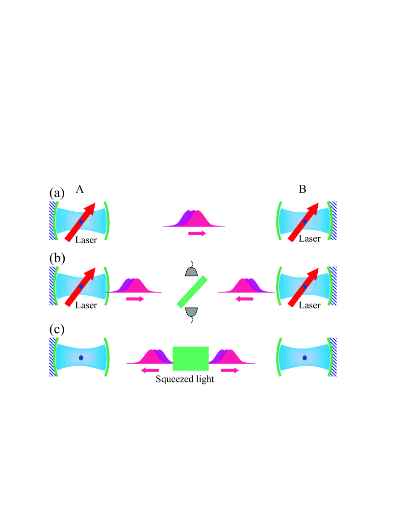
Figure 1: Schemes for entanglement creation over long distances: (a) Entanglement is created by the emission and subsequent absorption of a photon; (b) A detection of a photon projects the atoms in an entangled state; (c) Both cavities are driven by a common source of two–mode squeezed light. In steady state, the atoms become entangled.

Let us consider two two–level atoms, A and B, confined in two identical cavities, which are separated by a certain distance. The cavities are driven by an external source of two–mode squeezed light [see Fig. 1(c)]. Assuming that the bandwidth of the squeezed light is larger than the cavity damping rate $\kappa$, the evolution of the atoms–plus–cavity modes density operator, $\rho$, can be described using standard methods GardinerZoller by the following master equation

$$\frac{d\rho}{dt}=-i[H_{a}+H_{b},\rho]+({\cal L}_{\rm cav}+{\cal L}_{\rm at}^{a}+{\cal L}_{\rm at}^{b})\rho.$$ (1)

Here $H_{a}=g_{a}(a\sigma_{a}^{+}+a^{\dagger}\sigma_{a}^{-})$ describes the resonant interaction of atom A with the corresponding cavity mode, where $a$ is the mode annihilation operator and $\sigma_{a}^{+}=(\sigma_{a}^{-})^{\dagger}=|e\rangle_{a}\langle g|$, with $|g\rangle$ and $|e\rangle$ denoting the ground and excited atomic states note . Spontaneous emission $|e\rangle_{a}\to|g\rangle_{a}$ is described by the usual Liouvillian ${\cal L}_{\rm at}^{a}$ GardinerZoller , which is proportional to the spontaneous emission rate $\Gamma$. The terms $H_{b}$ and ${\cal L}_{\rm at}^{b}$ are analogously given. Finally, the interaction between the cavity modes and the squeezed light is given by

$${\cal L}_{\rm cav}\rho = \kappa(N+1)\sum_{\alpha=a,b}(\alpha\rho\alpha^{\dagger}-\alpha^{\dagger}\alpha\rho)$$ (2)

$$+\kappa N\sum_{\alpha=a,b}(\alpha^{\dagger}\rho\alpha-\alpha\alpha^{\dagger}\rho)$$

$$+\kappa M(2a\rho b+2b\rho a-2ba\rho-2ab\rho)+h.c.,$$

where $h.c.$ denotes hermitian conjugate. Here, $N$ and $M$ characterized the two–mode squeezed vacuum and fulfil $M\leq N(N+1)^{1/2}$. In the following we will concentrate in the case $g_{a}=g_{b}:=g$ since the formulas are considerably simplified. The effects for the case $g_{a}\neq g_{b}$ will be analyzed at the end.

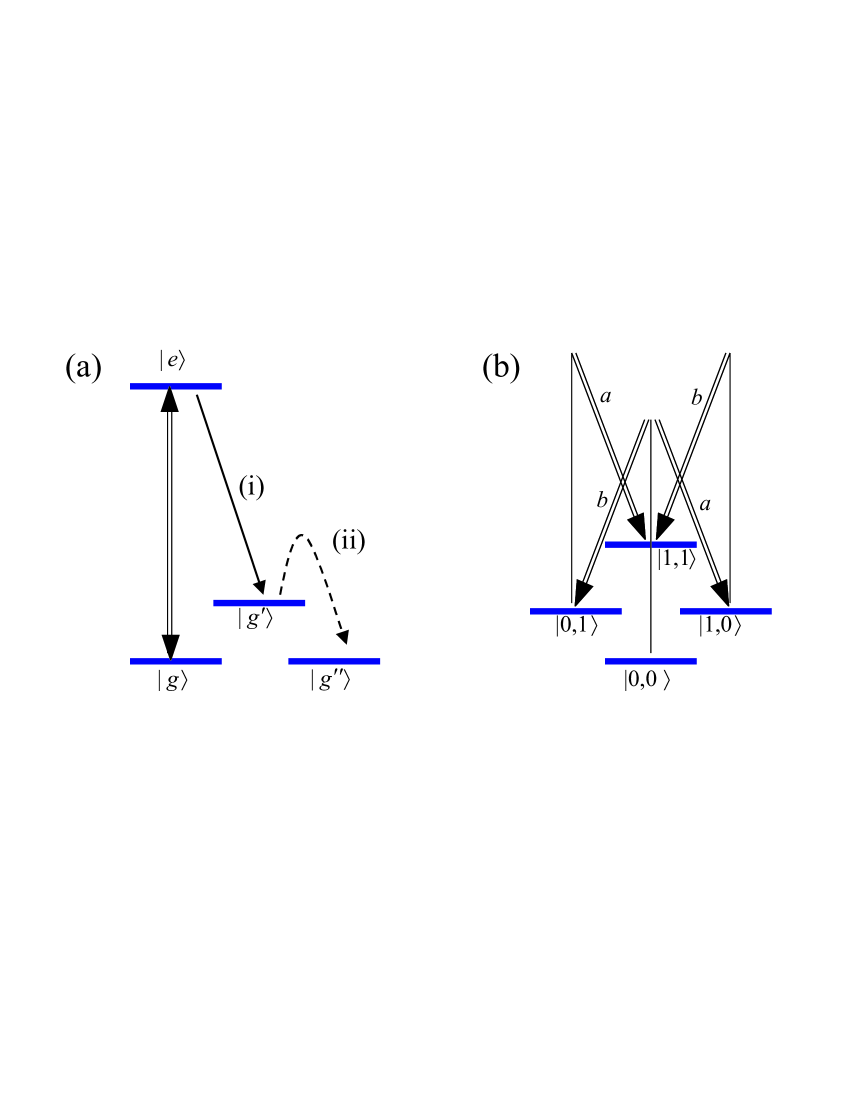
Figure 2: Atomic level schemes. Double lines indicates coupling to cavity modes and single lines to lasers: (a) Levels $|g\rangle$ and $|e\rangle$ are used for entanglement creation; level $|g^{\prime}\rangle$ is used to store the qubit once the entanglement has been created; level $|g^{\prime\prime}\rangle$ is used for entanglement concentration. (b) The four internal ground levels are coupled to two cavity modes ($a$ and $b$) by Raman transitions as indicated.

Let us first consider the ideal case in which $\Gamma=0$ and perfect squeezing

$$M=[N(N+1)]^{1/2}.$$ (3)

We can define new annihilation operators as $\tilde{a}=(N+1)^{1/2}a+N^{1/2}b^{\dagger}$ and $\tilde{b}=(N+1)^{1/2}b+N^{1/2}a^{\dagger}$, so that Eq. (1) can be rewritten as

$$\frac{d\rho}{dt}=-i[\tilde{H}_{a}+\tilde{H}_{b},\rho]+\tilde{\cal L}_{\rm cav}\rho,$$ (4)

where now

$$\tilde{H}_{a} = g(\tau_{a}^{+}\tilde{a}+\tilde{a}^{\dagger}\tau_{a}^{-}),$$ (5a)

$$\tilde{H}_{b} = g(\tau_{b}^{+}\tilde{b}+\tilde{b}^{\dagger}\tau_{b}^{-}),$$

$$\tilde{\cal L}_{\rm cav}\rho = \kappa\sum_{\alpha=\tilde{a},\tilde{b}}(\alpha\rho\alpha^{\dagger}-\alpha^{\dagger}\alpha\rho),$$ (5b)

with $\tau_{a,b}^{+}=(\tau_{a,b}^{-})^{\dagger}=(N+1)^{1/2}\sigma_{a,b}^{+}-N^{1/2}\sigma_{b,a}^{-}$. Solving master equation (4) seems to be a difficult task. However, one can easily determine the steady state, which is given by

$$|\Psi\rangle=\left(\sqrt{\frac{N+1}{2N+1}}|g\rangle_{a}|g\rangle_{b}+\sqrt{\frac{N}{2N+1}}|e\rangle_{a}|e\rangle_{b}\right)|0\rangle_{\tilde{a}}|0\rangle_{\tilde{b}},$$ (6)

where $|0\rangle_{\tilde{a},\tilde{b}}$ are the vacuum states of the new modes $\tilde{a}$ and $\tilde{b}$, respectively. This is a pure state, which in the limit $N\gg 1$ tends to a maximally entangled state. For a realistic value of $N\sim 1$ one still obtains a state with a large entanglement of formation (EoF) $E(\Psi)\sim 0.92$.

After the creation of the state (6), one should simultaneously switch off the squeezing source and transfer the excited state $|e\rangle$ of both atoms to some other internal ground state $|g^{\prime}\rangle$ using a laser, in order to avoid spontaneous emission [Fig. 2(a), (i)]. Once this is done, a maximally entangled state can be created as follows [Fig. 2(a), (ii)]. In each of the atoms, a radio frequency (or two–photon Raman) pulse is applied which transforms $|g^{\prime}\rangle\to cos\theta|g^{\prime}\rangle+\sin\theta|g^{\prime\prime}\rangle$, where $|g^{\prime\prime}\rangle$ is an auxiliary internal ground state, while the state $|g\rangle$ is not affected by the pulse. Then, the state $|g^{\prime\prime}\rangle$ is detected in both atoms using the quantum jump technique. If the outcome is negative, one can easily show that the atomic state will be projected onto a state proportional to $|g\rangle_{a}|g\rangle_{b}+|g^{\prime}\rangle_{a}|g^{\prime}\rangle_{b}$ if one chooses $\cos(\theta)=[(N+1)/N]^{1/4}$. Note that this measurement corresponds to a generalized measurement but in which the role of the ancilla is taken by the auxiliary level $|g^{\prime\prime}\rangle$, i.e. no extra atoms are required. The success probability depends on the value of $N$, but after a sufficiently large number of trials, a maximally entangled state can be prepared for any value of $N>0$.

In practice, there will be several physical phenomena which will distort the atomic entanglement in steady state. In the following, we will evaluate the effect of the most important sources of imperfection.

In order to analyze the non–ideal situation in which $\Gamma\neq 0$ and $M<[N(N+1)]^{1/2}$, we consider the limit $g\sqrt{N+1},\Gamma\ll\kappa$. Then, we can eliminate the cavity mode by generalizing the procedure presented in Cirac2 . We define $\sigma:={\rm tr}_{a,b}(\rho)$, so that

$$\frac{d\sigma}{dt}={\cal L}_{1}\rho+{\cal L}_{\rm at}^{a}\sigma+{\cal L}_{\rm at}^{b}\sigma,$$ (7)

where ${\cal L}_{1}(\rho)=-ig{\rm tr}_{a,b}(a[\sigma_{a}^{+},\rho]-h.c.)+a\leftrightarrow b$. On the other hand, integrating formally Eq. (1), and substituting the result in (7) one can check that in the limit $\kappa t\gg 1$, the dominant contribution is given by the term coming from

$$\rho(t)\simeq\int_{0}^{t}d\tau e^{{\cal L}_{\rm cav}\tau}{\cal L}_{2}[\rho(t-\tau)],$$ (8)

where ${\cal L}_{2}(\rho)=-ig([a,\rho\sigma_{a}^{+}]-h.c.)+a\leftrightarrow b$. Using that $e^{{\cal L}_{\rm cav}\tau}([a,R])=e^{-\kappa\tau}[a,e^{{\cal L}_{\rm cav}\tau}R]$ we see that the integrand will vanish for times $\kappa\tau\gg 1$, so that we can extend the limit of the integral to infinity. Moreover, since after the time $t$ the cavity mode will be driven to its steady state, $\rho_{ss}$, which fulfills ${\cal L}_{\rm cav}(\rho_{ss})=0$, we can replace $e^{{\cal L}_{\rm cav}\tau}\rho(t-\tau)\to\sigma(t)\otimes\rho_{ss}$. This procedure amounts to performing the standard Born–Markov approximations GardinerZoller , but here we have that the bath itself (cavity mode) undergoes a dissipative dynamics. After some lengthy algebra we obtain

$$\dot{\sigma} = \frac{\gamma}{2}(n+1)\sum_{\alpha=a,b}(\sigma_{\alpha}^{-}\sigma\sigma_{\alpha}^{+}-\sigma_{\alpha}^{+}\sigma_{\alpha}^{-}\sigma)$$ (9)

$$+\frac{\gamma}{2}n\sum_{\alpha=a,b}(\sigma_{\alpha}^{+}\sigma\sigma_{\alpha}^{-}-\sigma_{\alpha}^{-}\sigma_{\alpha}^{+}\sigma)$$

$$+\gamma m(\sigma_{a}^{-}\sigma\sigma_{b}^{-}+\sigma_{b}^{-}\sigma\sigma_{a}^{-}-\sigma_{b}^{-}\sigma_{a}^{-}\sigma-\sigma_{a}^{-}\sigma_{b}^{-}\sigma)$$

$$+h.c.$$

Here

$$\gamma = \frac{g^{2}}{\kappa}(2+\epsilon),\quad\epsilon:=\Gamma\kappa/(g^{2})$$ (10a)

$$n = N(1+\epsilon/2)^{-1},\quad m=-M(1+\epsilon/2)^{-1}.$$ (10b)

The interpretation of master equation (9) is straightforward. It describes the interaction of the two atoms with a common squeezed reservoir in which the squeezing parameters are renormalized due to the presence of spontaneous emission. The steady state solution only depends on $n$ and $m$, and can be easily determined. In fact, for $\Gamma=0$ and perfect squeezing we recover the steady state (6), as expected. Instead of analyzing our results in terms of $n$ and $m$, it is more convenient to analyze them in terms of the physical parameters $\epsilon$ and $N$, choosing (3). Note that it is always possible to find an $\epsilon$, and an $N$ and $M$ fulfilling (3), which give any prescribed values of $n$ and $m$, so that the effects of imperfect squeezing can be directly read off from our analysis.

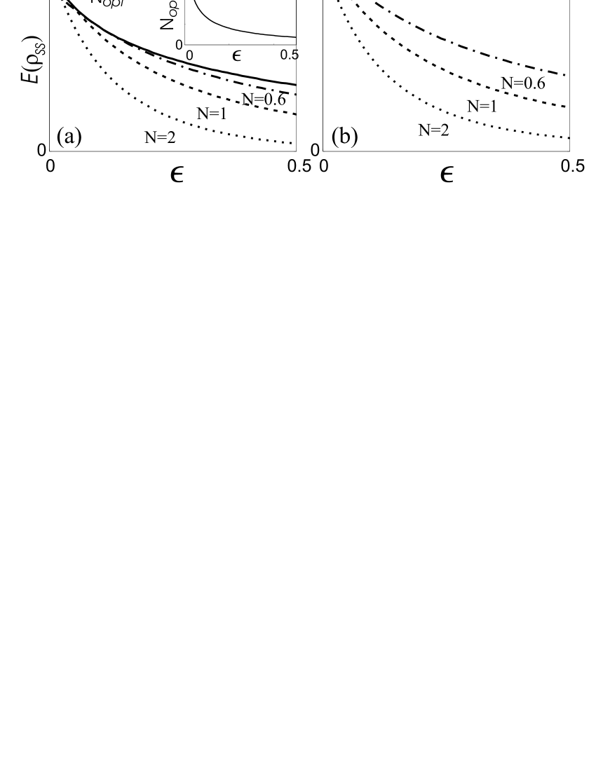
Figure 3: EoF of the atoms in steady state as a function of the parameter $\epsilon$ and various values of $N$: (a) Without generalized measurement; (b) With generalized measurement. The solid line indicates the optimal value and the insert gives the $N$ for which the EoF is optimal.

In Fig. [3(a)] we have plotted the atomic EoF of the steady state as a function of $\epsilon$ for various values of $N$. The most important aspect is that for $\epsilon\neq 0$ increasing the squeezing does not necessarily lead to an increase in the EoF. For each value of $\epsilon$ we have determined the best choice of $N$, which is shown in the insert. For realistic parameters $\epsilon\lesssim 0.1$ the best choice of $N$ is around $0.6$, leading to an EoF of $0.638$. In Fig. [3(b)] we have plotted the results when the filtering measurement described above is performed. Here we see that the achievable entanglement significantly increases. For example, for $\epsilon=0.1$ one obtains $0.775$.

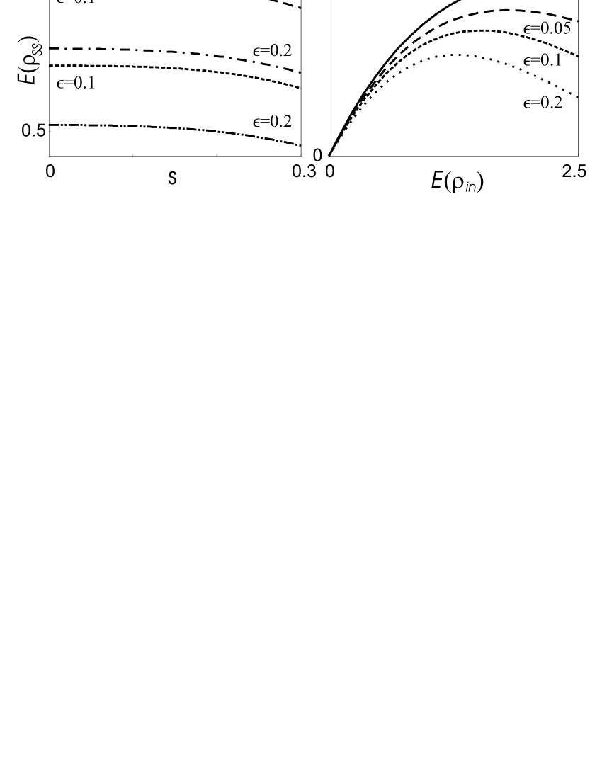
Figure 4: (a) EoF of the atoms in steady state as a function of the parameter $s$, for $N=0.5$. Upper (lower) two curves correspond to the case with (without) measurement after preparation; (b) EoF of the atomic state as a function of the one corresponding to the squeezed state.

In Fig. [4(a)] we have analyzed the effects of the imprecision in the position of the atoms noteLDL . To this aim, we have first extended our analysis to the case $g_{a}=g\cos(\theta_{a})\neq g_{b}=g\cos(\theta_{b})$, by deriving a master equation analogous to (9). We have then averaged the density operator corresponding to the steady state with respect to $\theta_{a}$ and $\theta_{b}$, with a weight function $p(\theta)\propto\exp[-\theta^{2}/(2s^{2})]$. We have plotted the resulting EoF as a function of $s$, which measures the experimental uncertainty in the position of the ion. The figure shows that this uncertainty does not have dramatic effects in the EoF, as long as the position of the particle is not far from the antinode of the cavity mode standing wave.

As mentioned in the introduction, with this scheme we are transforming the continuous variable entanglement contained in the squeezed vacuum state of the incident light into discrete (qubit) entanglement. In Fig. [(4(b)] we have analyzed the efficiency of this process. We have plotted the achieved EoF as a function of the EoF contained in the squeezed state for various values of $\epsilon$. The transfer is more efficient for low values of $N$, something that can be attributed to the fact that only two Schmidt coefficients are relevant for the two–mode squeezed state.

An important aspect of our scheme is that it can be scaled up to build a quantum communication network or quantum repeaters. The idea is to embed two (or more) atoms in each cavity, and to use two modes in each of them. Atoms A1 and B2 can interact with modes $a_{1}$ and $b_{2}$ in their respective cavities, which in turn are driven by two–mode squeezed light. Atoms B1 and C2 can also become entangled in a similar way by interacting with modes $b_{1}$ and $c_{2}$, respectively. In the ideal case, after the entanglement is created, a measurement in atoms B1 and B2 will yield an entangled state between atoms A1 and C2. In the presence of imperfections, the entanglement will be degraded every time we perform one of these operations (i.e. as we try to extend the entanglement over longer distances). In order to avoid this problem, one can use other auxiliary atoms in each cavity and perform entanglement purification as it is required to build a quantum repeater repeaters .

In the case of a small number of modes, it is possible to perform these experiments with a single atom per cavity and without having to perform joint measurements. This is not possible with two–level atoms, since it is known that in that case there is a maximum amount of entanglement that it can share with two neighboring atoms Duer . This problem can be circumvented by using several internal states, since in that case it is indeed possible that one atom shares two ebits with two other atoms. For example, one may take the atomic scheme of Fig. 2(b). We have renamed the internal state since then it is simpler to understand the scheme. Two cavity modes are used, that connect pairs of levels with the help of off–resonant laser beams in Raman configuration. Now, let us consider that we have three atoms A, B, C, in three different cavities. The atoms in A and C have the same configuration as before, whereas the atom in cavity B has the one indicated in Fig. 2(b). The Hamiltonian, after adiabatically eliminating the excited state of atom B has the form

$$H=g(\sigma_{a}^{+}a+\sigma_{b_{1}}^{+}b_{1}+\sigma_{b_{2}}^{+}b_{2}+\sigma_{c}^{+}c)+h.c.$$ (11)

Here, $\sigma_{a,c}^{+}$ are defined as before, whereas

$$\sigma_{b_{1}}^{+} = |1,0\rangle_{B}\langle 0,0|+|1,1\rangle_{B}\langle 0,1|,$$ (12a)

$$\sigma_{b_{2}}^{+} = |0,1\rangle_{B}\langle 0,0|+|1,1\rangle_{B}\langle 1,0|.$$ (12b)

Now, if modes $a$ and $b_{1}$ and modes $c$ and $b_{2}$ are driven by two independent sources of squeezed light, it is easy to check that under ideal conditions ($\Gamma=0$ and perfect squeezing) the atomic steady state is

$$|\Psi\rangle_{ss} = \frac{N+1}{2N+1}|g\rangle_{A}|0,0\rangle_{B}|g\rangle_{C}+\frac{N}{2N+1}|e\rangle_{A}|1,1\rangle_{B}|e\rangle_{C}$$

$$+ \frac{\sqrt{N(N+1)}}{2N+1}(|g\rangle_{A}|0,1\rangle_{B}|e\rangle_{C}+|e\rangle_{A}|1,0\rangle_{B}|g\rangle_{C}).$$

In the limit $N\gg 1$ this state contains two ebits, one between A and B and another between B and C. Alternatively, an appropriate measurement in B will produce a maximally entangled state between A and C with certain probability. This scheme can be easily generalized to a larger number of nodes. However, as mentioned above, the role of the imperfections will be important and one eventually needs to consider several atoms in each cavity to purify the obtained entanglement.

In conclusion, we have shown that atoms can get entangled by interacting with a common source of squeezed light. The continuous variable entanglement can, in this way, be transformed in discrete one in steady state. Local measurements result in a more efficient entanglement creation. Given the experimental progress in trapping atoms inside cavities Kimble3 and the successful experiments on coupling squeezed light into a cavity Kimble , the present scheme may become a very robust alternative to current methods to construct quantum networks for quantum communication.

This work has been supported in part by the Kompetenznetzwerk Quanteninformationsverarbeitung der Bayerischen Staatsregierung and by the EU IST projects ”RESQ” and ”QUPRODIS”. After completion of this work we have learned of a related problem but using an atomic Raman configurationParkins3 .

References

- (1) H.J. Briegel, W. Dür, J.I. Cirac, P. Zoller, Phys. Rev. Lett. 81, 5932 (1998).
- (2) R. Cleve, D. Gottesman, and H.-K. Lo, Phys. Rev. Lett. 83, 648 (1999)
- (3) see, for example, R. Cleve and H. Buhrman, Phys. Rev. A 56, 1201 (1997).
- (4) J. S. Bell, ”Speakable and Unspeakable in Quantum Mechanics”, Cambridge University Press, 1989.
- (5) J. I. Cirac, P. Zoller, H. J. Kimble, and H. Mabuchi, Phys. Rev. Lett. 78, 3221 (1997).
- (6) A.S. Parkins and H.J. Kimble, Phys. Rev. A 61, 052104 (2000).
- (7) C. W. Gardiner, P. Zoller, ” Quantum Noise” Springer, 2000.
- (8) G. Giedke and J. I. Cirac, Phys. Rev. A 66, 032316 (2002); J. Eisert, S. Scheel, and M. B. Plenio, Phys. Rev. Lett. 89, 137903 (2002).
- (9) S. Clark, A. Peng, M. Gu, and A. S. Parkins, quant-ph/0307064.
- (10) C. Cabrillo, J. I. Cirac, P. Garcia-Fernandez and P. Zoller, Phys. Rev. A 59, 1025 (1999).
- (11) M. B. Plenio, S. F. Huelga, A. Beige, and P. L. Knight, Phys. Rev. A 59, 2468 (1999).
- (12) One can also entangle atomic ensembles using this method: L.-M. Duan, M. D. Lukin, J. I. Cirac, P. Zoller, Nature 414, 413 (2001).
- (13) C. W. Gardiner, Phys. Rev. Lett. 56, 1917 (1986); S. Clark and S. Parkins, J. Opt. B: Quantum Semiclass. Opt. 5, 145 (2003).
- (14) N. Ph. Georgiades, E. S. Polzik, K. Edamatsu, H. J. Kimble, and A. S. Parkins, Phys. Rev. Lett. 75, 3426 (1995).
- (15) J. McKeever, J. R. Buck, A. D. Boozer, A. Kuzmich, H.-C. Nägerl, D. M. Stamper-Kurn, and H. J. Kimble Phys. Rev. Lett. 90, 133602 (2003); A. Kuhn, M. Hennrich, G. Rempe, Phys. Rev. Lett. 89, 067901 (2002).
- (16) Note that one can also use Raman transition for this purpose [see, for example, S. G. Clark and A. S. Parkins, Phys. Rev. Lett. 90, 047905 (2003)]. However, one has to use extra lasers to avoid the effects of AC Stark shifts and the method becomes less efficient.
- (17) J. I. Cirac, Phys. Rev. A 46, 4354 (1992).
- (18) We are assuming that the atoms are confined in the LDL, so that their motion does not play any role. It may be interesting to detune the cavity mode to the red to enhance sideband cooling.
- (19) W. Dür, G. Vidal and J. I. Cirac, Phys. Rev. A 62, 062314 (2000); W. K. Wootters, Contemporary Mathematics 305, 299 (2002).
- (20) S. Clark and A. S. Parkins (priviate communication).