Intertwining technique for the one-dimensional stationary Dirac equation

Abstract

The technique of differential intertwining operators (or Darboux transformation operators) is systematically applied to the one-dimensional Dirac equation. The following aspects are investigated: factorization of a polynomial of Dirac Hamiltonians, quadratic supersymmetry, closed extension of transformation operators, chains of transformations, and finally particular cases of pseudoscalar and scalar potentials. The method is widely illustrated by numerous examples.

, ,

1 Introduction

In recent times a growing interest to applications of supersymmetric quantum mechanics (SUSY QM) in different fields of theoretical and mathematical physics is noticed. Thus, it has been applied to generate new families of exactly solvable potentials [1]–[4], to study ordinary symmetries of the set of Riccati equations [5], and also to analyse a new kind of symmetry of ordinary differential equations, called translational invariance with respect to Darboux transformations [6]. As it has been understood after the work by Andrianov et al. [7], SUSY QM (first introduced by Witten [8] as a toy model in Quantum Field Theory) is basically equivalent to a method of finding solutions of a differential equation from the known solutions of another equation just by applying to them a differential operator. This approach was studied for the first time by Darboux [9] and is known nowadays as the method of Darboux transformations. Its most famous applications are related with nonlinear equations of mathematical physics [10] and inverse scattering problem [11]–[13]. Another formulation of the same method is due to Schrödinger and it is known as factorization method in quantum mechanics [14, 15].

Though this method is widely used for Schrödinger-like equations, its application to systems of equations, and in particular to the Dirac system, is studied much less. Probably the first paper where a differential-matrix intertwining operator for the Dirac equation is constructed is due to Anderson [16]. It deals with component equations for the transformation operator. For the particular case of a pseudoscalar potential this author has found rather complicated equations defining the transformation operator. This might be the reason why his method has not received much popularity. In another paper [17] Stahlhofen applies a general theorem proved in [10] to study transparent pseudoscalar potentials for the Dirac equation, obtaining and analysing new kind of potentials with eigenvalues embedded in the continuous spectrum. Although there is not a new technique in this paper, it illustrates the idea that similar methods may find unexpected applications. We notice also the papers [18, 19] (for a review see [10]) where ad hoc Darboux transformation operators are constructed for some systems of differential equations, and the paper [20] where the authors use differential transformation operators for finding particular solutions of the inverse problem for a regular Dirac operator.

We would like to remark that the technique of integral intertwining operators is well-known in the method of inverse quantum scattering [21] (see also [22]), but differential-matrix intertwiners have been found only quiet recently [20, 23].

In this paper we give a consistent introduction to differential-matrix intertwining operators for the one-dimensional stationary Dirac equation (Section 2) and study their main properties. We shall show that every property of a differential intertwiner for the Schrödinger equation finds its counterpart in the case of the Dirac equation. Thus, in Section 3 we prove a theorem about factorization of a polynomial of Dirac operators by means of Darboux transformation operators, which serves as a basis for establishing a hidden quadratic supersymmetry underlying our method (Section 6). In Section 4 we show that despite the fact that our transformation operators have nontrivial kernels, a one-to-one correspondence between the spaces of solutions of the initial and transformed equations is possible. Section 5 is devoted to analysing transformation operators as acting in a Hilbert space. In Section 7 we study chains of transformations and establish relativistic analogs of Crum determinant formulas [24]. Sections 8 and 9 are devoted to studying particular cases of pseudoscalar and scalar potentials. Our method is widely illustrated by numerous examples given in Section 10. Finally, in Section 11 we draw some conclusions and give an outlook of future works.

2 Darboux transformation for the Dirac equation

Consider the one-dimensional stationary Dirac equation

$$h_{0}\psi=E\psi\,.$$ (1)

Here $h_{0}=\gamma\partial_{x}+V_{0}$, $\gamma=i\sigma_{2}$, $\sigma_{2}$ is a Pauli matrix, $\partial_{x}\equiv d/dx$, $V_{0}$ is $2\times 2$ real symmetric potential matrix and the function $\psi$ is a two-component vector (we shall call it spinor), $\psi=(\psi_{1},\psi_{2})^{t}$ (the superscript “$t$” meaning the transpose). We do not indicate the interval where the real variable $x$ falls, because our constructions are independent of this interval.

Suppose we know all solutions $\psi$ to Eq. (1) and we want to solve a similar equation for another Hamiltonian $h_{1}$ defined by the potential $V_{1}$. The problem of finding eigenfunctions $\varphi$ of the Hamiltonian $h_{1}$,

$$h_{1}\varphi=E\varphi,$$ (2)

can be reduced to the problem of finding a transformation operator (see e.g. [22]), also called intertwiner [5], defined by the equation

$$Lh_{0}=h_{1}L\,.$$ (3)

It follows from here that the function $\varphi=L\psi$ is a solution (maybe trivial) of Eq. (2). Here and in the following we shall suppose that all operators act in the space of spinors with sufficiently smooth (i.e. infinitely differentiable) components. In this paper we restrict ourselves to differential transformation operators. From this point of view let us consider the simplest differential transformation operator

$$L=A\partial_{x}+B\,.$$ (4)

Here $A$ and $B$ are $2\times 2$ matrices with $x$-dependent entries. Similar transformation operator for the Schrödinger equation leads (see e.g. [25]) to the transformation investigated for the first time by Darboux [9]), and therefore it is usually called “Darboux transformation operator”. In this context it is natural to call any differential transformation operator Darboux transformation operator [25].

Using the intertwining relation (3), and assuming the linear independence of derivative operators $\partial_{x}^{k}$, $k=0,1,\ldots$, we are led to the following system of equations for $A$, $B$ and $V_{1}$:

$$A\gamma-\gamma A=0\,,$$ (5)

$$AV_{0}-V_{1}A+B\gamma-\gamma B-\gamma A_{x}=0\,,$$ (6)

$$AV_{0x}+BV_{0}-\gamma B_{x}-V_{1}B=0\,.$$ (7)

The subscript $x$ denotes the derivative with respect to $x$, e.g. $A_{x}=dA/dx$, and the matrix $A_{x}$ is composed of the first derivatives of the elements of the matrix $A$.

The Eq.(5) may be considered as a restriction imposed on the matrix $A$: two of its four elements may be chosen arbitrarily, and the other two should be found in terms of the previous ones. The Eq. (6) defines the potential difference $D=V_{1}-V_{0}$:

$$D=(AV_{0}-V_{0}A+B\gamma-\gamma B-\gamma A_{x})A^{-1}\,.$$ (8)

We are supposing that $A$ is an invertible matrix for all values of $x$. From (7) we will find $B$. To integrate this equation we first change the dependent variable $B$ in favor of a new variable $\Omega$: $B=A\Omega$. Thus, upon using (8) we obtain from (7) the equation for $\Omega$

$$(V_{0}-\gamma\Omega)_{x}+\Omega V_{0}-V_{0}\Omega+(\gamma\Omega-\Omega\gamma)\Omega=0.$$ (9)

This equation can be considered as the derivative of a relativistic analog of the Riccati equation that appears when similar calculations are carried out on the Schrödinger equation. Eq. (9) can be linearized and integrated by a similar substitution: $\Omega=-{\mathcal{U}}_{x}\,{\mathcal{U}}^{-1}$. After such a calculation we get

$$[\,{\mathcal{U}}^{-1}(V_{0}{\mathcal{U}}+\gamma{\mathcal{U}}_{x})\,]_{x}=0\,,$$ (10)

where ${\mathcal{U}}$ is supposed to be everywhere invertible. Now, denoting by $\Lambda$ a matrix integration constant, we get the equation for ${\mathcal{U}}$:

$$\gamma{\mathcal{U}}_{x}+V_{0}{\mathcal{U}}={\mathcal{U}}\Lambda\,.$$ (11)

The matrix $\Lambda$ should be taken hermitian.

We notice that (11) is very similar to the initial Dirac Eq. (1). The single difference is that $\psi$ is a spinor and $E$ is a number, while ${\mathcal{U}}$ and $\Lambda$ are matrices. Nevertheless, if solutions of (1) are known we can immediately solve (11).

Since the matrix $\Lambda$ is hermitian it always can be reduced to a diagonal form. Therefore let us take $\Lambda$ to be diagonal

$$\Lambda=\left(\begin{array}[]{cc}\lambda_{1}&0\\ 0&\lambda_{2}\end{array}\right).$$ (12)

If we now choose ${\mathcal{U}}=(u_{1},u_{2})$, where spinors $u_{1}$ and $u_{2}$ are solutions of (1) with the eigenvalues $\lambda_{1}$ and $\lambda_{2}$ respectively,

$$h_{0}u_{1,2}=\lambda_{1,2}u_{1,2}\,,$$

then ${\mathcal{U}}$ is a solution of (11). We will choose the spinors $u_{1}$ and $u_{2}$ real, which is always possible if we suppose $\lambda_{1}$ and $\lambda_{2}$ to be real.

Once the matrix ${\mathcal{U}}$ is known, the transformation operator $L$ and the transformed potential $V_{1}$ are defined up to the matrix $A$

$$L=A[\partial_{x}-{\mathcal{U}}_{x}\,{\mathcal{U}}^{-1}]\,,$$

$$V_{1}=A(V_{0}+\Omega\gamma-\gamma\Omega-\gamma A^{-1}A_{x})A^{-1}\,.$$

The matrix $A$ remains arbitrary provided it satisfies the condition (5). Nevertheless, remark that the simple gauge transformation $\varphi=A\widetilde{\varphi}$ reduces it to the identity. Therefore, without loss of generality we can take $A=I$, where $I$ is $2\times 2$ unit matrix. Now the operator $L$ has its simplest possible form

$$L=\partial_{x}-{\mathcal{U}}_{x}\,{\mathcal{U}}^{-1}\,,$$ (13)

which is the relativistic extension of the well known Darboux transformation operator for the Schrödinger equation (see e.g. [25]). For the transformed potential we get

$$V_{1}=V_{0}+D,\quad D=\Omega\gamma-\gamma\Omega,\quad\Omega=-{\mathcal{U}}_{x}\,{\mathcal{U}}^{-1}\,.$$ (14)

We observe here that the transformation operator and the transformed potential are completely defined by the matrix-function ${\mathcal{U}}$. Therefore, we will call it transformation function.

Using Eq. (11) one can express ${\mathcal{U}}_{x}$ in terms of ${\mathcal{U}}$ and $V_{0}$. This gives us another representation for the transformed potential

$$V_{1} = -\gamma V_{0}\gamma+\widetilde{D},$$ (15)

$$\widetilde{D} = u\Lambda u^{-1}+\gamma u\Lambda u^{-1}\gamma=(\lambda_{1}-\lambda_{2})\Delta\left(\begin{array}[]{cc}d_{1}&d_{2}\\ d_{2}&-d_{1}\end{array}\right)\,,$$ (18)

where

$$d_{1}=u_{11}u_{22}+u_{12}u_{21}\,,\qquad d_{2}=u_{21}u_{22}+u_{11}u_{12}\,,$$ (19)

$\Delta=(\det{\mathcal{U}})^{-1}$ and $u_{ij}$, $i,j=1,2$, are the entries of the matrix ${\mathcal{U}}$. Similar transformations applied to the formula (13) yield

$$\varphi=L\psi=\gamma({\mathcal{U}}\Lambda{\mathcal{U}}^{-1}-E)\psi\,.$$ (20)

This formula is equivalent to (13) provided $L$ acts on an eigenfunction of $h_{0}$ with the eigenvalue $E$.

Before going further, it is necessary to point out a couple of simple but relevant comments.

Remark 1

Given a hamiltonian $h_{0}=\gamma\partial_{x}+V_{0}$, if the hermitian potential matrix $V_{0}(x)$ is symmetric, then it can be reduced by a smooth orthogonal transformation [22] to the form

$$V_{0}(x)=p_{0}(x)\sigma_{3}+q_{0}(x)\sigma_{1},$$ (21)

where $\sigma_{1},\sigma_{3}$ are Pauli matrices, known as a canonical representation of $V_{0}$. Therefore, in the following we shall use only this canonical representation for the Dirac potentials.

Remark 2

Any potential of the form (21) has the properties

$$\gamma V_{0}\gamma=V_{0}\,,\qquad\gamma V_{0}+V_{0}\gamma=0\,.$$ (22)

Note that the operator $L$ has a nontrivial kernel, $L\,{\mathcal{U}}=0$, i.e. $\mbox{ker}L$ is a two dimensional linear space spanned by the spinors $u_{1}$ and $u_{2}$. This means that the set of the spinors $L\psi$, when $\psi$ runs through the whole space of solutions of the initial equation, may in general not coincide with the whole space of the solutions of the transformed equation. In Section 3 we shall show that despite this fact a one-to-one correspondence between the spaces of solutions of the equations (1) and (2) may be established.

3 One-to-one correspondence between the spaces of solutions

To define the Dirac Hamiltonian and the transformation operator we have not used the notion of the Hilbert space and an inner product is not defined in the space of spinors. Nevertheless, we need operators adjoint to given ones. Therefore in the space of operators we are working we shall define the operation of conjugation in a formal way. Namely, we will require $\partial_{x}^{+}=-\partial_{x}$, $(AB)^{+}=B^{+}A^{+}$, $i^{+}=-i$ (where $i$ is the imaginary unity), and if $A$ is a matrix, $A^{+}$ is its hermitian conjugate in the usual sense (i.e., it is obtained from $A$ by transposing and taking the complex conjugation). Moreover, for a given invertible matrix ${\mathcal{U}}$ we will assume that the operations of taking the inverse and adjoint commute, i.e.,

$$({\mathcal{U}}^{+})^{-1}=({\mathcal{U}}^{-1})^{+}\,.$$ (23)

It is easy to see that the Dirac operators $h_{0}$ and $h_{1}$ are self-adjoint. Therefore, the adjoint intertwining relation reads

$$h_{0}L^{+}=L^{+}h_{1}\,.$$ (24)

This means that the operator $L^{+}$ is also a transformation operator and it realizes the transformation in the opposite direction, from the solutions of (2) to solutions of (1). But as we will show below, it is not an inverse of $L$.

It is well known that for any fixed value of the energy the Dirac system (1) has two linearly independent solutions. As in the case of the Schrödinger equation, if we know one of them, $\psi$ with eigenvalue $E$, the other solution $\widetilde{\psi}$ with the same eigenvalue can be found by a quadrature. In this way we get the spinors $\widetilde{u}_{1}$ and $\widetilde{u}_{2}$ with eigenvalues $\lambda_{1}$ and $\lambda_{2}$. They do not belong to the space $\mbox{ker}L$ and hence $v_{1,2}=L\widetilde{u}_{1,2}$ are nontrivial solutions of the transformed equation with the eigenvalues $\lambda_{1,2}$. We will find them next.

For this purpose we need a counterpart of the Wronskian which, like in the case of the Schrödinger equation, may be defined as a function of two solutions $\psi$ and $\widetilde{\psi}$ corresponding to the same eigenvalue $E$, which is independent of the variable $x$. Using the adjoint form of the Eq. (1), we easily find

$$(\widetilde{\psi}^{+}\gamma\psi)_{x}=\widetilde{\psi}_{1}\psi_{2x}+\widetilde{\psi}_{1x}\psi_{2}-\widetilde{\psi}_{2}\psi_{1x}-\widetilde{\psi}_{2x}\psi_{1}=0\,,$$ (25)

which means that

$$W(\widetilde{\psi},\psi):=\widetilde{\psi}^{+}\gamma\psi=\widetilde{\psi}_{1}\psi_{2}-\widetilde{\psi}_{2}\psi_{1}=\mbox{constant}\,.$$ (26)

Hence, the function $W(\widetilde{\psi},\psi)$ we just defined can play the role of the Wronskian. The solutions $\psi$ and $\widetilde{\psi}$ can always be chosen such that the constant that appears in (26) is equal to one.

The Dirac system with a canonical potential $V_{0}=p_{0}\sigma_{3}+q_{0}\sigma_{1}$, written in terms of the components $\psi_{1}$ and $\psi_{2}$ of the spinor $\psi=(\psi_{1},\psi_{2})^{t}$, has the form:

$$\psi_{2x}+p_{0}\psi_{1}+q_{0}\psi_{2}=E\psi_{1}\,,\qquad-\psi_{1x}+q_{0}\psi_{1}-p_{0}\psi_{2}=E\psi_{2}\,.$$ (27)

The same system for the components of the spinor $\widetilde{\psi}=(\widetilde{\psi}_{1},\widetilde{\psi}_{2})^{t}$ is

$$\widetilde{\psi}_{2x}+p_{0}\widetilde{\psi}_{1}+q_{0}\widetilde{\psi}_{2}=E\widetilde{\psi}_{1}\,,\qquad-\widetilde{\psi}_{1x}+q_{0}\widetilde{\psi}_{1}-p_{0}\widetilde{\psi}_{2}=E\widetilde{\psi}_{2}\,.$$ (28)

If now we eliminate the function $q_{0}$ from the last equations of (27) and (28) we obtain

$$\psi_{1}\widetilde{\psi}_{1x}-\widetilde{\psi}_{1}\psi_{1x}=p_{0}+E\,,$$ (29)

where we have used formula (26). From here, assuming that $\psi_{1}$ is not identically zero, we easily find

$$\widetilde{\psi}_{1}=\psi_{1}\int_{x_{0}}^{x}\frac{p_{0}+E}{\psi_{1}^{2}}\,dx\,.$$ (30)

Formula (26) gives us the second component of the spinor $\widetilde{\psi}$:

$$\widetilde{\psi}_{2}=\frac{\widetilde{\psi}_{1}\psi_{2}}{\psi_{1}}-\frac{1}{\psi_{1}}\,.$$ (31)

If $\psi_{1}(x)\equiv 0$ then, for a nontrivial spinor $\psi=(\psi_{1},\psi_{2})^{t}$, $\psi_{2}(x)$ is not identical null, and the following alternative formulae should be used:

$$\widetilde{\psi}_{2}=\psi_{2}\int_{x_{0}}^{x}\frac{E-p_{0}}{\psi_{2}^{2}}\,dx\,,\qquad\widetilde{\psi}_{1}=\frac{\widetilde{\psi}_{2}\psi_{1}}{\psi_{2}}+\frac{1}{\psi_{2}}\,.$$ (32)

Now, we can apply (20) to the eigenspinors $\widetilde{u}_{1,2}$ with the eigenvalues $\lambda_{1,2}$ which gives us the action of $L$ on the matrix $\widetilde{\mathcal{U}}=(\widetilde{u}_{1},\widetilde{u}_{2})$. After some simple algebra we get

$$L\,\widetilde{\mathcal{U}}=(\lambda_{2}-\lambda_{1}){\mathcal{V}}\,,$$ (33)

$${\mathcal{V}}=({\mathcal{U}}^{+})^{-1}\,.$$ (34)

Hence, the matrix ${\mathcal{V}}$ satisfies the equation $h_{1}{\mathcal{V}}={\mathcal{V}}\Lambda$, $\Lambda=\mbox{diag}(\lambda_{1},\lambda_{2})$. It is composed of the spinors $v_{1}$ and $v_{2}$, ${\mathcal{V}}=(v_{1},v_{2})$, satisfying the Dirac equation with the potential $V_{1}$, $h_{1}v_{1,2}=\lambda_{1,2}v_{1,2}$. Two other eigenspinors of $h_{1}$, $\widetilde{v}_{1}$ and $\widetilde{v}_{2}$, with respective eigenvalues $\lambda_{1}$ and $\lambda_{2}$, $h_{1}\widetilde{v}_{1,2}=\lambda_{1,2}\widetilde{v}_{1,2}$, may be found with the help of the same formulas (30)–(32), applied this time to the transformed equation.

Hence, we have established a one-to-one correspondence between the spaces of solutions of the equations (1) and (2). For any $E\neq\lambda_{1},\lambda_{2}$ the operators $L$ and $L^{+}$ realize this correspondence; if $E=\lambda_{1,2}$ the correspondence can be assured by the mapping ${\mathcal{U}}_{1,2}\leftrightarrow\widetilde{\mathcal{V}}_{1,2}$, $\widetilde{\mathcal{U}}_{1,2}\leftrightarrow{\mathcal{V}}_{1,2}$, considered as a linear mapping.

As a final remark of this Section, we notice that $L^{+}{\mathcal{V}}=0$, meaning that $\widetilde{\mathcal{U}}\in{\rm ker}L^{+}L$. In addition, the operator $L^{+}$ expressed in terms of ${\mathcal{V}}$ reads as $L^{+}=-\partial_{x}-({\mathcal{U}}^{+})^{-1}{\mathcal{U}}^{+}_{x}=-\partial_{x}+{\mathcal{V}}_{x}{\mathcal{V}}^{-1}$. This means that if we interchange the role of the initial and final equations, the function ${\mathcal{V}}$ becomes the transformation function for the transformation operator of the type (13), taken with the opposite sign and realizing the transformation in the opposite direction, a fact that we already mentioned. Moreover, for the transformed equation the function $\widetilde{\mathcal{V}}$ plays the same role that $\widetilde{\mathcal{U}}$ plays for the initial equation. This implies that, according to (33), $L^{+}{\mathcal{V}}=(\lambda_{1}-\lambda_{2}){\mathcal{U}}$. Taking into consideration the fact that ${\mathcal{U}}\in{\rm ker}L$, we find that in one hand $\widetilde{\mathcal{V}}\in{\rm ker}LL^{+}$. On the other hand,  $\{{\mathcal{U}},\widetilde{\mathcal{U}}\}\in{\rm ker}(h_{0}-\lambda_{1})(h_{0}-\lambda_{2})$, and $\{{\mathcal{V}},\widetilde{\mathcal{V}}\}\in{\rm ker}(h_{1}-\lambda_{1})(h_{1}-\lambda_{2})$. Hence, we see that

$${\rm ker}(h_{0}-\lambda_{1})(h_{0}-\lambda_{2})={\rm ker}L^{+}L={\rm span}({\mathcal{U}},\widetilde{\mathcal{U}})$$ (35)

and

$${\rm ker}(h_{1}-\lambda_{1})(h_{1}-\lambda_{2})={\rm ker}LL^{+}={\rm span}({\mathcal{V}},\widetilde{\mathcal{V}})\,.$$ (36)

From these properties, we can suspect that the operator $L^{+}L$ coincides with $(h_{0}-\lambda_{1})(h_{0}-\lambda_{2})$ and the operator $LL^{+}$ coincides with $(h_{1}-\lambda_{1})(h_{1}-\lambda_{2})$. These facts will be proved in the next Section.

4 Factorization property of Darboux transformations

Before establishing the main result of this Section, we need first to prove some auxiliary relations.

Proposition 1

For any real $2\times 2$ matrix $A$ the following formula holds: $\gamma A+A^{+}\gamma={\rm tr}A\,\gamma$.

Proof. Since the set of matrices $\left\{I,\gamma,\sigma_{1},\sigma_{3}\right\}$ is complete in the space of $2\times 2$ matrices, any such a matrix may be presented in the form

$$A=aI+b_{1}\sigma_{1}+b_{2}\gamma+b_{3}\sigma_{3}$$

and therefore $\mbox{tr}A=2a$. The statement of the Proposition follows from the fact that the Pauli matrices anticommute. $\Box$

Lemma 1

The matrix ${\mathcal{U}}$ defined as ${\mathcal{U}}:=(u_{1},u_{2})$, where $u_{1}$ and $u_{2}$ are real eigenspinors of $h_{0}$ (with eigenvalues $\lambda_{1}$ and $\lambda_{2}$ respectively) chosen such that ${\mathcal{U}}$ is non-degenerate, satisfies the following relationship:

$$U:={\mathcal{U}}_{x}\,{\mathcal{U}}^{-1}-({\mathcal{U}}_{x}\,{\mathcal{U}}^{-1})^{+}=-(\lambda_{1}+\lambda_{2})\gamma\,.$$ (37)

Proof. The equation for ${\mathcal{U}}$ (11) together with (23) implies

$$({\mathcal{U}}^{+})^{-1}{\mathcal{U}}_{x}^{+}=-V_{0}\gamma+({\mathcal{U}}^{+})^{-1}\Lambda{\mathcal{U}}^{+}\gamma\,.$$ (38)

From here it follows the relation for $U$ as given in (37)

$$U=\gamma V_{0}+V_{0}\gamma-\gamma{\mathcal{U}}\Lambda{\mathcal{U}}^{-1}-({\mathcal{U}}\Lambda{\mathcal{U}}^{-1})^{+}\gamma\,,$$ (39)

which, after taking into account Remark 2, can be rewritten in the equivalent form

$$U=-[\gamma{\mathcal{U}}\Lambda{\mathcal{U}}^{-1}-({\mathcal{U}}\Lambda{\mathcal{U}}^{-1})^{+}\gamma]\,.$$ (40)

The statement of the Lemma 1 follows from this equation, Proposition 1, and the following equality: $\rm{tr}\,({\mathcal{U}}\Lambda{\mathcal{U}}^{-1})=\mbox{tr}\,\Lambda=\lambda_{1}+\lambda_{2}$. $\Box$

Proposition 2

The following relationships hold for the matrices ${\mathcal{U}}$, chosen as in Lemma 1, and $\Lambda$, given in (12):

$${\mathcal{U}}_{xx}{\mathcal{U}}^{-1}=V_{0}^{2}+\gamma V_{0x}-{\mathcal{U}}\Lambda^{2}{\mathcal{U}}^{-1}\,,$$ (41)

$$\Lambda^{2}-(\lambda_{1}+\lambda_{2})\Lambda=-\lambda_{1}\lambda_{2}I\,.\quad$$ (42)

Proof. The first one is a differential implication of the Eq. (11). Indeed, if we take the derivative of this equation and replace the first derivative of ${\mathcal{U}}$ using the same Eq. (11), we get

$$\gamma{\mathcal{U}}_{xx}+V_{0x}{\mathcal{U}}+V_{0}\gamma V_{0}{\mathcal{U}}-V_{0}\gamma{\mathcal{U}}\Lambda=\gamma V_{0}{\mathcal{U}}\Lambda-\gamma{\mathcal{U}}\Lambda^{2}\,.$$ (43)

Now we use the formulae

$$V_{0}\gamma V_{0}{\mathcal{U}}=-\gamma V_{0}^{2}{\mathcal{U}}\,,\qquad V_{0}\gamma{\mathcal{U}}\lambda=-\gamma V_{0}{\mathcal{U}}\Lambda\,,$$ (44)

which are direct implications of (22), and rewrite (43) as follows:

$$\gamma{\mathcal{U}}_{xx}+V_{0x}{\mathcal{U}}-\gamma V_{0}^{2}{\mathcal{U}}=-\gamma{\mathcal{U}}\Lambda^{2}.$$ (45)

Formula (41) is now evident.

Formula (42) may be proved straightforwardly, by computing explicitly its left hand side using (12). $\Box$

We establish and prove now the main result of this Section.

Theorem 1

Darboux transformation operator $L$ given in (13) and its formally adjoint $L^{+}$, constructed with the help of the matrix ${\mathcal{U}}:=(u_{1},u_{2})$, where $u_{1}$ and $u_{2}$ are real eigenspinors of $h_{0}$ (with eigenvalues $\lambda_{1}$ and $\lambda_{2}$ respectively) chosen such that ${\mathcal{U}}$ is non-degenerate, factorize the following polynomial of the Dirac Hamiltonians $h_{0}$ and $h_{1}$:

$$L^{+}L = (h_{0}-\lambda_{1}I)(h_{0}-\lambda_{2}I)\,,$$ (46)

$$LL^{+} = (h_{1}-\lambda_{1}I)(h_{1}-\lambda_{2}I)\,.$$ (47)

Proof. Let us consider the superposition $L^{+}L$. Using (13) and after some simple algebraic rearrangements, one gets

$$L^{+}L=-\partial_{x}^{2}+U\partial_{x}+{\mathcal{U}}_{xx}\,{\mathcal{U}}^{-1}-U{\mathcal{U}}_{x}\,{\mathcal{U}}^{-1}.$$ (48)

We now replace here $U$ by the right hand side of the formula (37) and use Eq. (41) obtaining

$$\begin{array}[]{rcl}L^{+}L=&-&\partial_{x}^{2}+V_{0}^{2}+\gamma V_{0x}-{\mathcal{U}}\Lambda^{2}{\mathcal{U}}^{-1}\\[4.30554pt] &-&(\lambda_{1}+\lambda_{2})(\gamma\partial_{x}+V_{0})-{\mathcal{U}}[\Lambda^{2}-(\lambda_{1}+\lambda_{2})\Lambda]{\mathcal{U}}^{-1}\,.\end{array}$$ (49)

Formula (46) follows from here, Eq. (42), and the equalities $\gamma\partial_{x}+V_{0}=h_{0}$ and $-\partial_{x}^{2}+V_{0}^{2}+\gamma V_{0x}=h_{0}^{2}$.

To prove formula (47), we act with $L$ on the Eq. (46), and take into account the intertwining relation (3). As a result, we obtain

$$LL^{+}L\psi=(h_{1}-\lambda_{1}I)(h_{1}-\lambda_{2}I)L\psi\,.$$ (50)

The last equation means that (47) is valid for any $\varphi=L\psi$ and it remains to prove it for the spinors which can not be represented in this form. But we know that such spinors are eigenspinors of $h_{1}$, either with the eigenvalue $\lambda_{1}$ or with $\lambda_{2}$. For these spinors both right and left hand sides of (47) are zero, since the spaces $\mbox{ker}\,LL^{+}$ and $\mbox{ker}\,(h_{1}-\lambda_{1}I)(h_{1}-\lambda_{2}I)$ coincide, as we already commented in (36). $\Box$

As a consequence of this Theorem, taking into account (18) and Remark 2, summarized in Eq. (22), the Darboux transformations keep unchanged the canonical representation of a potential.

To conclude this Section, we notice that for the case $\lambda_{1}=-\lambda_{2}=\lambda_{0}$ Eq. (46) takes the form

$$L^{+}L=(h_{0}-\lambda_{0})(h_{0}+\lambda_{0})=(h_{0}^{2}-\lambda_{0}^{2}),$$

a result that was previously reported in [16] for a scalar potential.

5 Darboux transformation operators in a Hilbert space

Let us consider a Dirac Hamiltonian $h_{0}$ defined in a dense domain $D$ of the Hilbert space $H=L^{2}({\mathbb{R}})\otimes{\mathbb{C}}^{2}$, $D\subset H$ with the inner product

$$\langle\Psi|\Phi\rangle:=\int_{-\infty}^{\infty}\psi^{\dagger}(x)\varphi(x)dx\,.$$ (51)

Here $\psi^{\dagger}(x)=(\psi_{1}^{*}(x),\psi_{2}^{*}(x))$. We shall denote the elements of the Hilbert space by capital symbols and we shall keep small symbols for the coordinate representation of the corresponding spinors. We shall suppose that the differential expression $\gamma\partial_{x}+V_{0}$, initially defined in a dense subset $D\subset L^{2}({\mathbb{R}})\otimes{\mathbb{C}}^{2}$ of sufficiently smooth functions, has a self-adjoint extension with domain of definition $\overline{D}$, which we shall denote by the same symbol $h_{0}$. In this case the system of eigenspinors $|\Psi_{E}\rangle\in D$, $h_{0}|\Psi_{E}\rangle=E|\Psi_{E}\rangle$, is complete in $H$. This means that there exists a measure $\rho(E)$ such that the following completeness condition takes place

$$\int d\rho(E)\,|\Psi_{E}\rangle\langle\Psi_{E}|=1\,.$$ (52)

This equation should be understood in a week sense, i.e., it is equivalent to

$$\int d\rho(E)\,\langle\Phi_{n}|\Psi_{E}\rangle\langle\Psi_{E}|\Phi_{m}\rangle=\delta_{n,m}\,,\quad n,m=0,1,\ldots,$$ (53)

where $|\Phi_{n}\rangle$, $n=0,1,\ldots$ is an orthonormal basis in $H$. In coordinate representation the kets $|\Psi_{E}\rangle$ are reduced to the smooth spinors $\psi_{E}$. Therefore the action of $L$ on them is well-defined. Let us consider the following family of spinors

$$|\Phi_{E}\rangle=N_{E}^{-1}L|\Psi_{E}\rangle\,,\quad\forall|\Psi_{E}\rangle\in D,$$ (54)

where $N^{2}_{E}=(E-\lambda_{1})(E-\lambda_{2})$. It is easy to see that these spinors are elements of $H$ if $N^{2}_{E}>0$. Indeed, they are eigenspinors of $h_{1}$: $h_{1}|\Phi_{E}\rangle=E|\Phi_{E}\rangle$. Therefore, taking into account the factorization property (46), we can define the action of $L^{+}$ on the spinor $|\Phi_{E}\rangle$

$$L^{+}|\Phi_{E}\rangle=N_{E}^{-1}L^{+}L|\Psi_{E}\rangle=N_{E}|\Psi_{E}\rangle\,.$$ (55)

Remark that the right hand side of (51) is nothing but the sum of two integrals with respect to Lebesque measure on the real line. Therefore, when $L$ acts on eigenspinors of $h_{0}$ and $L^{+}$ acts on these of $h_{1}$, the adjoint operation formally introduced at the begining of Section 3 coincides with the adjoint with respect to the inner product (51). As a result, for all $\lambda_{1}<\lambda_{2}$ such that the interval $(\lambda_{1},\lambda_{2})$ does not contain spectral points of $h_{0}$, we have

$$\langle\Phi_{E}|\Phi_{E}\rangle=N^{-2}_{E}\langle L\Psi_{E}|L\Psi_{E}\rangle=N^{-2}_{E}\langle\Psi_{E}|L^{+}L\Psi_{E}\rangle=\langle\Psi_{E}|\Psi_{E}\rangle\,.$$ (56)

This result means that if $E>\lambda_{2}$ or $E<\lambda_{1}<\lambda_{2}$ is such that $E\in\mbox{spec}(h_{0})$, then it also happens that $E\in\mbox{spec}(h_{1})$. The inverse statement is in general not valid. Hence, to find the whole spectrum of $h_{1}$ it remains to analyse the values $\lambda_{1}$ and $\lambda_{2}$ only. Here, several possibilities can take place. Let us consider two real numbers $\tilde{\mu}$ and $\mu$, $\tilde{\mu}<\mu$, such that the interval $(\tilde{\mu},\mu)$ is a spectral gap of $h_{0}$, for instance the gap between the positive and negative parts of the spectrum, if any. Then, the main posibilities are the following:

• If $\mu$ is a level of the discrete spectrum, then one can take $\lambda_{2}=\mu$, $\tilde{\mu}<\lambda_{1}<\lambda_{2}$, and $u_{2}=\psi_{\mu}$.

  • If, in addition, there exists a linear combination of $v_{1}$ and $\widetilde{v}_{1}$, $\varphi=c_{1}v_{1}+c_{2}\widetilde{v}_{1}$ (we recall that $v_{1}$ ($\widetilde{v}_{1}$) is the first column of the matrix ${\mathcal{V}}$ ($\widetilde{\mathcal{V}}$)), such that $\varphi\in H$, then the level $E=\mu$ will not be present in the spectrum of $h_{1}$, but the new discrete level $E=\lambda_{1}$ will appear.

  • If the last condition is not satisfied, the spectrum of $h_{1}$ will coincide with the spectrum of $h_{0}$, except for one level $E=\mu$, which is missing in the spectrum of $h_{1}$.

• If both $\lambda_{1}$ and $\lambda_{2}$ fall inside the interval $(\tilde{\mu},\mu)$, $\tilde{\mu}<\lambda_{1}<\lambda_{2}<\mu$, then the following posibilities arise:

  • The spectrum of $h_{1}$ totally coincides with the spectrum of $h_{0}$.

  • One discrete level is created at $E=\lambda_{1}$

  • One discrete level is created at $E=\lambda_{2}$.

  • Two new levels are created at $E=\lambda_{1}$ and $E=\lambda_{2}$.

Since the functions $\Psi_{E}$ are smooth enough, we know the action of $L$ not only on these spinors, but also on any linear combination of them of the form

$$|\Psi\rangle=\int d\rho(E)C(E)|\Psi_{E}\rangle,$$ (57)

where $C(E)$ is a finite function over $\mathbb{R}$, i.e., a function with a compact support. The set of spinors (57) is a linear space that we will denote in the sequel by ${\mathcal{L}}_{0}$. We notice that it is dense in $H$. The image of the space ${\mathcal{L}}_{0}$ under the action of the operator $L$ consists of the spinors

$$|\Phi\rangle=\int d\rho(E)N_{E}C(E)|\Phi_{E}\rangle\,.$$ (58)

This new set will be denoted by ${\mathcal{L}}_{1}$. The operator $L^{+}$, being a linear operator, is defined for all $|\Phi\rangle\in{\mathcal{L}}_{1}$. Moreover, the following equality holds

$$\langle L\Psi|\Phi\rangle=\langle\Psi|L^{+}\Phi\rangle\,,\qquad\forall|\Psi\rangle\in{\mathcal{L}}_{0}\,,\quad\forall|\Phi\rangle\in{\mathcal{L}}_{1}\,.$$ (59)

Nevertheless, this does not mean that the operator $L^{+}$ is adjoint to $L$ with respect to the inner product in $H$. To find such an operator one has to specify correctly its domain of definition. We shall not look for this domain. Instead we shall give a closed extension $\bar{L}$ of the operator $L$ and then find its adjoint $\bar{L}^{\dagger}$ with respect to the inner product in $H$.

For simplicity, let us suppose that $h_{1}$ is completely isospectral with $h_{0}$. (If this is not the case, the reasonings are similar, but it will be necessary to specify the spaces where the operators act on.) In this case the set of functions (54) is another basis in the same space $H$ and the operator

$$U=\int d\rho(E)|\Phi_{E}\rangle\langle\Psi_{E}|$$ (60)

realizes an unitary mapping of $H$ onto itself,

$$U^{-1}=U^{\dagger}=\int d\rho(E)|\Psi_{E}\rangle\langle\Phi_{E}|\,,$$ (61)

provided the vectors $|\Psi_{E}\rangle$ are orthonormal. Consider now the following operators

$$\bar{L} = \int d\rho(E)N_{E}|\Phi_{E}\rangle\langle\Psi_{E}|\,,$$ (62)

$$\bar{L}^{\dagger} = \int d\rho(E)N_{E}|\Psi_{E}\rangle\langle\Phi_{E}|\,,$$ (63)

It is not difficult to specify their domains of definition. For this purpose we introduce the self-adjoint operator $g_{0}=(h_{0}-\lambda_{1})(h_{0}-\lambda_{2})$, wich has the following spectral decomposition

$$g_{0}=\int d\rho(E)N_{E}^{2}|\Psi_{E}\rangle\langle\Psi_{E}|\,.$$ (64)

We shall suppose the parameters $\lambda_{1}$ and $\lambda_{2}$ to be such that $g_{0}$ is positive definite. Then, the spectral decomposition of its square root is

$$g_{0}^{1/2}=\int d\rho(E)N_{E}|\Psi_{E}\rangle\langle\Psi_{E}|\,.$$ (65)

It follows now that

$$\|\bar{L}\Psi\|^{2}=\|g_{0}^{1/2}\Psi\|^{2}=\int d\rho(E)N_{E}^{2}|\langle\Psi|\Psi_{E}\rangle|^{2}\,.$$ (66)

This means that the domain of definition of $\bar{L}$ coincides with that of $g_{0}^{1/2}$ and consists of all $\psi\in H$ such that the integral in the right-hand side of (66) converges. The domain of definition of $\bar{L}^{\dagger}$ coincides with that of the operator $g_{1}^{1/2}$ where $g_{1}=(h_{1}-\lambda_{1})(h_{1}-\lambda_{2})$ is also positive definite.

From formulae (62) and (63) it follows that the operator $\bar{L}^{\dagger}$ is the adjoint of $\bar{L}$ with respect to the inner product, the domains of definition of $\bar{L}$ and $\bar{L}^{\dagger}$ being well specified. Moreover, $\bar{L}^{\dagger\dagger}=\bar{L}$. This implies [26, 27] that the operator $\bar{L}$ is closed. Expressions (62)–(63) give quasispectral representations of the closed operators $\bar{L}$ and $\bar{L}^{\dagger}$.

From (62)–(63) it also follows that $\bar{L}\psi_{E}=L\psi_{E}=N_{E}\varphi_{E}$ and $\bar{L}^{\dagger}\varphi_{E}=L^{+}\varphi_{E}=N_{E}\psi_{E}$. This means that $\bar{L}$ is the closed extension of the operator $L$, and $\bar{L}^{\dagger}$ is the closed extension of the operator $L^{+}$, when the domains ${\mathcal{L}}_{0}$ and ${\mathcal{L}}_{1}$ are taken as their initial domains of definition.

From the spectral decomposition of the operators $g_{0}^{1/2}$ (65) and $g_{1}^{1/2}$,

$$g_{1}^{1/2}=\int dpN_{p}|\varphi_{p}\rangle\langle\varphi_{p}|\,,$$

one obtains the following representations for $\bar{L}$ and $\bar{L}^{+}$:

$$\bar{L}=Ug_{0}^{1/2}=g_{1}^{1/2}U\,,\quad\bar{L}^{\dagger}=g_{0}^{1/2}U^{\dagger}=U^{\dagger}g_{1}^{1/2}\,.$$

Such representations are known as polar decompositions or canonical representations of closed operators (see for example [27, 28]).

Let us consider now bounded operators

$$M=\int d\rho(E)N_{E}^{-1}|\Phi_{p}\rangle\langle\Psi_{E}|\,,\qquad M^{\dagger}=\int d\rho(E)N_{E}^{-1}|\Psi_{p}\rangle\langle\Phi_{E}|\,,$$

defined in $H$. It is not difficult to see that both $M\bar{L}^{\dagger}$ and $M^{\dagger}\bar{L}$ are unit operators in $H$. Using the spectral resolutions of the operators $g_{0}^{-1/2}$ and $g_{1}^{-1/2}$,

$$g_{0}^{-1/2}=\int d\rho(E)N_{E}^{-1}|\Psi_{E}\rangle\langle\Psi_{E}|\,,\qquad g_{1}^{-1/2}=\int d\rho(E)N_{E}^{-1}|\Phi_{E}\rangle\langle\Phi_{E}|\,,$$

one derives the polar decompositions of the operators $M$ and $M^{\dagger}$:

$$M=Ug_{0}^{-1/2}=g_{1}^{-1/2}U\,,\qquad M^{\dagger}=g_{0}^{-1/2}U^{\dagger}=U^{\dagger}g_{1}^{-1/2}\,.$$

It is easily seen that these operators factorize the inverses of $g_{0}$ and $g_{1}$: $M^{\dagger}M=g_{0}^{-1}$, $MM^{\dagger}=g_{1}^{-1}$.

As a final remark of this Section, we would like to notice that the space $H$ can be obtained as a closure of the linear space ${\mathcal{L}}_{0}$ of all finite linear combinations of the functions $|\Phi_{E}\rangle=L|\Psi_{E}\rangle$ with respect to the norm generated by the inner product (51). The set of functions of the form $|\Phi\rangle=\bar{L}|\Psi\rangle$, when $|\Psi\rangle$ runs through the whole domain of definition of the operator $\bar{L}$ (i.e., the domain of definition of the operator $\sqrt{g_{0}}$, $D({\sqrt{g_{0}}})$), can not give the whole space $H$. Nevertheless, if one defines a new inner product in ${\mathcal{L}}_{1}$, $\langle\Phi_{a}|\Phi_{b}\rangle_{1}\equiv\langle L\Psi_{a}|L\Psi_{b}\rangle=\langle\Psi_{a}|g_{0}|\Psi_{b}\rangle$, $|\Psi_{a,b}\rangle\in{\mathcal{L}}_{0}$, $|\Phi_{a,b}\rangle\in{\mathcal{L}}_{1}$, then the closure of ${\mathcal{L}}_{1}$ with respect to the norm generated by this inner product coincides with the set $|\Phi\rangle=\bar{L}|\Psi\rangle$, $|\Psi\rangle\in D({\sqrt{g_{0}}})$. This space is embedded in $H$.

6 Supersymmetry

As it has been mentioned in the Introduction, supersymmetric transformations in the non-relativistic quantum mechanics are basically equivalent to Darboux transformations for the Schrödinger equation. This equivalence is based on two properties of the Darboux transformation: (a) the intertwining relations and (b) the factorization of the Hamiltonians, similar to that established in Section 4.

In the case of the Dirac equation we started from the intertwining relation and proved the factorization properties. Therefore, every property giving rise to the supersymmetry of the Schrödinger equation also takes place for the Dirac equation. Moreover, the transformation operators are well-defined in the Hilbert space $L^{2}({\mathbb{R}})\otimes{\mathbb{C}}^{2}$. Therefore, in order to show the supersymmetric character of our approach we can proceed in the same way as in the nonrelativistic case.

To begin, let us introduce the following $4\times 4$ matrices

$${\mathcal{H}}\equiv\left(\begin{array}[]{cc}h_{0}&0\\ 0&h_{1}\\ \end{array}\right)\,,\quad{\mathcal{Q}}^{+}=\left(\begin{array}[]{cc}0&L^{+}\\ 0&0\\ \end{array}\right)\,,\quad{\mathcal{Q}}=\left(\begin{array}[]{cc}0&0\\ L&0\\ \end{array}\right)\,.$$ (67)

It is easily seen that, in one side, the two commutation relations

$$[{\mathcal{Q}},{\mathcal{H}}]=[{\mathcal{Q}}^{+},{\mathcal{H}}]=0$$ (68)

are equivalent to the intertwining relations (3) and (24). On the other side, the anticommutation relations

$$\{{\mathcal{Q}},{\mathcal{Q}}^{+}\}\equiv{\mathcal{Q}}{\mathcal{Q}}^{+}+{\mathcal{Q}}^{+}{\mathcal{Q}}=({\mathcal{H}}-\lambda_{1}I)({\mathcal{H}}-\lambda_{2}I)$$ (69)

are equivalent to the factorizations (46) and (47), while

$${\mathcal{Q}}^{2}=({\mathcal{Q}}^{+})^{2}=0\,.$$ (70)

Remark that relations (68)–(70) are those of a quadratic deformation of the superalgebra $sqm(2)$, inherent to the usual supersymmetric quantum mechanics [8]. This quadratic superalgebra cannot be seen directly from the Dirac equation, and therefore we associate it with a hidden supersymmetry. Let us also point out that a superalgebra similar to that of (68-70) can also be found in the non-relativistic context, when second order Darboux transformations are considered [29, 30].

7 Chains of Darboux transformations

The aim of this Section is to iterate the one-step transformations we have considered in previous sections. In order to accomplish this goal, we will rewrite first the formulas (13) and (14) in a form wich will be more appropriate for this purpose. Remark that the action of the operator $L$ to $\psi$ can be rewritten as follows

$$\varphi=L\psi=\psi_{x}-{\mathcal{U}}_{x}\,{\mathcal{U}}^{-1}\psi={\mathcal{U}}({\mathcal{U}}^{-1}\psi)_{x}\,.$$ (71)

Now, we will substitute the term in parentheses by the following expression

$${\mathcal{U}}^{-1}\psi=\frac{1}{W(f,g)}\left(\begin{array}[]{l}W(\psi,g)\\[4.30554pt] W(f,\psi)\end{array}\right),$$ (72)

where $W(f,g)=f^{t}\gamma g=f_{1}g_{2}-f_{2}g_{1}$ is the Wronskian for the Dirac equation that we introduced in Section 4, being $f$ and $g$ the spinors from wich the matrix ${\mathcal{U}}$ is composed: ${\mathcal{U}}=(f,g)$, $f=(f_{1},f_{2})^{t}$, $g=(g_{1},g_{2})^{t}$, and $h_{0}f=\lambda f,h_{0}g=\mu g$, i.e., $\Lambda={\rm diag}(\lambda,\mu)$. It can be established by a straightforward calculation that the derivative of (72) can be written as

$$({\mathcal{U}}^{-1}\psi)_{x}=\frac{1}{[W(f,g)]^{2}}\left(\begin{array}[]{l}W_{S}(W(f,g),W(\psi,g))\\[4.30554pt] W_{S}(W(f,g),W(f,\psi))\end{array}\right),$$ (73)

were $W_{S}(f,g)=fg^{\prime}-f^{\prime}g$ is the usual Wronskian. In the sequel we will use both, the prime and the subscript $x$, for denoting the derivative with respect to $x$; as usual, a multiple derivative of a function $f$ will be denoted as $f^{(n)}$.

After replacing $({\mathcal{U}}^{-1}\psi)_{x}$ for its expression in (73), one gets from (71) the desired form for $\varphi$:

$$\varphi=\frac{1}{W(f,g)}\left(\hskip 1.00006pt\left|\begin{array}[]{lll}f_{1}&g_{1}&\psi_{1}\\ f_{2}&g_{2}&\psi_{2}\\ f^{\prime}_{1}&g^{\prime}_{1}&\psi^{\prime}_{1}\end{array}\right|,\hskip 3.00003pt\left|\begin{array}[]{lll}f_{1}&g_{1}&\psi_{1}\\ f_{2}&g_{2}&\psi_{2}\\ f^{\prime}_{2}&g^{\prime}_{2}&\psi^{\prime}_{2}\end{array}\right|\hskip 1.00006pt\right)^{t}.$$ (74)

The symbols $\left|\begin{array}[]{cc}\cdot&\cdot\\ \cdot&\cdot\end{array}\right|$ are used to denote determinants. A similar calculation results in another representation of the transformed potential matrix $V_{1}$ given in (14):

$$V_{1}=V_{0}+[\gamma,D_{1}],$$ (75)

where the square brackets represent the commutator. The matrix $D_{1}$ is

$$D_{1}=\frac{1}{W(f,g)}\left(\begin{array}[]{ll}\left|\begin{array}[]{ll}f^{\prime}_{1}&g^{\prime}_{1}\\ f_{2}&g_{2}\end{array}\right|&\left|\begin{array}[]{ll}f_{1}&g_{1}\\ f^{\prime}_{1}&g^{\prime}_{1}\end{array}\right|\\[12.91663pt] \left|\begin{array}[]{ll}f^{\prime}_{2}&g^{\prime}_{2}\\ f_{2}&g_{2}\end{array}\right|&\left|\begin{array}[]{ll}f_{1}&g_{1}\\ f^{\prime}_{2}&g^{\prime}_{2}\end{array}\right|\end{array}\right).$$ (76)

In the next subsections we generalize the formulae (74)–(76) to a chain of $n$ consecutive transformations of the same type.

7.1 Transformation of spinors

Let us denote now by $L_{1\leftarrow 0}$ the first order operator intertwining $h_{0}$ and $h_{1}$, as given in (13), having the transformation function ${\mathcal{U}}_{1}$ with the eigenvalue $\Lambda_{1}=\mbox{diag}(\lambda_{1},\mu_{1})$, $\lambda_{1}\neq\mu_{1}$. Let ${\mathcal{U}}_{2}$ be a solution of (1) with $\Lambda_{2}=\mbox{diag}(\lambda_{2},\mu_{2})$, $\lambda_{2}\neq\mu_{2}$, $\left\{\lambda_{2},\mu_{2}\right\}\neq\left\{\lambda_{1},\mu_{1}\right\}$. The last condition, together with the non-degeneracy of ${\mathcal{U}}_{1}$, means the non-degeneracy of the matrix ${\mathcal{V}}_{2}=L_{1\leftarrow 0}{\mathcal{U}}_{2}$. The function ${\mathcal{V}}_{2}$ being an eigenfunction of $h_{1}$ may be chosen as the transformation function for the second transformation step.

The operator carrying out the second transformation will be denoted by $L_{2\leftarrow 1}$. It intertwines $h_{1}$ and $h_{2}$, the new potential given by the formula (14) in which the replacements $V_{0}\to V_{1}$, $V_{1}\to V_{2}$ and ${\mathcal{U}}\to{\mathcal{V}}_{2}$ are done. It follows from here that the second order operator

$$L_{2\leftarrow 0}=L_{2\leftarrow 1}L_{1\leftarrow 0}$$ (77)

intertwines $h_{0}$ and $h_{2}$ and realizes the transformation from $h_{0}$ directly to $h_{2}$, without using an intermediate potential $V_{1}$. It is completely defined by two transformation functions ${\mathcal{U}}_{1}$ and ${\mathcal{U}}_{2}$. It is clear that subsequent iterations give us an $n$th order transformation operator

$$L_{n\leftarrow 0}=L_{n\leftarrow n-1}\cdots L_{2\leftarrow 1}L_{1\leftarrow 0}\,,$$ (78)

realizing the transformation between the first $h_{0}$ and the last $h_{n}$ elements of the chain of Hamiltonians $h_{0},h_{1},\ldots,h_{n}$. The operator $L_{n\leftarrow 0}$ is defined by $n$ transformation functions ${\mathcal{U}}_{1},\ldots,{\mathcal{U}}_{n}$

$$h_{0}{\mathcal{U}}_{i}={\mathcal{U}}_{i}\Lambda_{i},\quad\Lambda_{i}=\mbox{diag}(\lambda_{i},\mu_{i})\,.$$ (79)

We shall derive now a compact formula for the eigenfunctions of the Hamiltonian $h_{n}$ (not necessary belonging to the Hilbert space). For the columns of the matrix ${\mathcal{U}}_{i}$ we introduce the notations $f_{i}=(f_{i1},f_{i2})^{t}$, $g_{i}=(g_{i1},g_{i2})^{t}$, so that ${\mathcal{U}}_{i}=(f_{i}\,,g_{i})$, $f_{i}$, $g_{i}$ being two-component vector-columns (spinors), and $h_{0}f_{i}=\lambda_{i}f_{i}$, $h_{0}g_{i}=\mu_{i}g_{i}$.

In order to obtain the formulas we are looking for, we need to introduce new notations. Let $W(f_{1},$ $g_{1},\ldots,f_{n},g_{n})$ be a $(2n)$th order determinant organized as follows. The first two rows of this determinant are composed of the components of the spinors $f_{1}$, $g_{1}$, …, $f_{n}$, $g_{n}$, the first line from the first components and the second line from the second components; any subsequent pairs of rows is the derivative of the previous pair. Thus, we can write

$$W(f_{1},g_{1},\ldots,f_{n},g_{n})\equiv W(f_{1},\ldots,g_{n})=\det(a_{i,j}),\ i,j=1,2,\ldots 2n\,,$$ (80)

where

$$\left.\begin{array}[]{ll}a_{2l-1,2m-1}=f^{(l-1)}_{m1},&a_{2l,2m-1}=f^{(l-1)}_{m2},\\[8.61108pt] a_{2l-1,2m}=g^{(l-1)}_{m1},&a_{2l,2m}=g^{(l-1)}_{m2},\end{array}\right\}$$ (81)

$l,m=1,\ldots,n$. Remember that $W(f_{1},g_{1},\ldots,f_{n},g_{n})$ is the determinant of an even order matrix.

We need also some odd order determinants. If we have the same set of $2n$ spinors $f_{i}$ and $g_{i}$, $i=1,\ldots,n$, plus an additional spinor $\psi=(\psi_{1},\psi_{2})^{t}$, then we can construct two different determinants of $(2n+1)$th order from the previous determinant (80): by adding a column composed of these spinors (using the procedure described above) and a row composed of the $n$th derivative of either the upper elements of the spinors $f_{1}$, $g_{1}$, …, $f_{n}$, $g_{n}$, $\psi$, or the lower elements of the spinors. In this way, we can get determinants of two kinds

$$W_{1}(f_{1},g_{1},\ldots,f_{n},g_{n},\psi) = \det(b_{i,j})\,,$$ (82)

$$W_{2}(f_{1},g_{1},\ldots,f_{n},g_{n},\psi) = \det(c_{i,j})\,,\quad i,j=1,2,\ldots 2n+1\,,$$ (83)

where $b_{i,j}=c_{i,j}=a_{i,j}$ when $i,j=1,\ldots,2n$, and

$$\left.\begin{array}[]{l}b_{2l-1,2n+1}=c_{2l-1,2n+1}=\psi^{(l-1)}_{1},\ l=1,\ldots,n;\\[4.30554pt] b_{2l,2n+1}=c_{2l,2n+1}=\psi^{(l-1)}_{2},\ l=1,\ldots,n;\\[4.30554pt] b_{2n+1,2m-1}=f^{(n)}_{m1},\ c_{2n+1,2m-1}=f^{(n)}_{m2},\ m=1,\ldots,n;\\[4.30554pt] b_{2n+1,2m}=g^{(n)}_{m1},\ c_{2n+1,2m-1}=g^{(n)}_{m2},\ m=1,\ldots,n;\\[4.30554pt] b_{2n+1,2n+1}=\psi^{(n)}_{1},\ c_{2n+1,2n+1}=\psi^{(n)}_{2}.\end{array}\right\}$$ (84)

Now, in order to prove the main result of this Section, we need the following auxiliary statements.

Lemma 2

The following equation takes place:

$$W_{S}\bigl{(}W(f_{1},g_{1},\ldots,f_{n},g_{n}),W(f_{1},g_{1},\ldots,f_{n},\psi)\bigr{)}=$$

$$\hskip 56.9055pt=W_{1}(f_{1},g_{1},\ldots,f_{n-1},g_{n-1},f_{n})W_{2}(f_{1},g_{1},\ldots,f_{n},g_{n},\psi)$$ (85)

$$\hskip 59.75095pt-W_{2}(f_{1},g_{1},\ldots,f_{n-1},g_{n-1},f_{n})W_{1}(f_{1},g_{1},\ldots,f_{n},g_{n},\psi)\,.$$

Proof. To prove the lemma we need first the following identity, which can be checked in [19]:

$$W^{\ell}_{\ell\ell}W^{\ell}_{jk}-W^{\ell}_{j\ell}W^{\ell}_{\ell k}=W^{\ell+1}_{jk}W_{\ell-1},$$ (86)

where

$$W^{\ell}_{jk}:=W_{1,2,\ldots,\ell-1,j;1,2,\ldots,\ell-1,k},\quad j,k>\ell,$$

$$W_{i_{1},i_{2},\ldots,i_{k},;j_{1},j_{2},\ldots,j_{k}}:=\det(y_{i_{m},j_{n}}),\quad m,n=1,\ldots,k,$$

and $y_{i_{m},j_{n}}$ are arbitrary.

Note first that the derivative of a determinant such as the one defined in (80) is the sum of two determinants of a similar structure. The difference is only either in the last row or in the next-to-last row. In the first case we obtain the determinant denoted by $R_{1}(f_{1},g_{1},\ldots,f_{n},g_{n})$ in which the last row is replaced by the $n$th derivative of the second elements of the spinors $f_{1}$, $g_{1}$, …, $f_{n}$, $g_{n}$ and in the second case we get the determinant denoted by $R_{2}(f_{1},g_{1},\ldots,f_{n},g_{n})$ in which the next-to-last row is replaced by the $n$th derivative of the first elements of the same spinors. To be more precise, we have the following

$$[W(f_{1},\ldots,g_{n})]^{\prime}=R_{1}(f_{1},g_{1},\ldots,f_{n},g_{n})+R_{2}(f_{1},g_{1},\ldots,f_{n},g_{n})\,,$$ (87)

where

$$R_{1}(f_{1},g_{1},\ldots,f_{n},g_{n})=\det(r^{1}_{i,j})\,,$$ (88)

$$R_{2}(f_{1},g_{1},\ldots,f_{n},g_{n})=\det(r^{2}_{i,j})\,,\quad i,j=1,2,\ldots 2n\,,$$ (89)

and

$$\left.\begin{array}[]{l}r^{1}_{i,j}=r^{2}_{i,j}=a_{i,j},\ \ i=1,\ldots,2n-2,\ j=1,\ldots,2n;\\[4.30554pt] r^{1}_{2n-1,2m-1}=f^{(n)}_{m1},\ r^{1}_{2n-1,2m}=g^{(n)}_{m1},\ \ m=1,\ldots,n;\\[4.30554pt] r^{2}_{2n,2m-1}=f^{(n)}_{m2},\ r^{2}_{2n,2m}=g^{(n)}_{m2},\ \ m=1,\ldots,n;\\[4.30554pt] r^{1}_{2n,j}=a_{2n,j},\ r^{2}_{2n-1,j}=a_{2n-1,j},\ \ j=1,\ldots,2n.\end{array}\right\}$$ (90)

The functions $a_{i,j}$ are defined in (81). The Lemma follows now from (86) and (87). $\Box$

Proposition 3

In what follows, we will need also the following identity

$$W_{1}(f_{1},g_{1},\ldots,f_{n-1},g_{n-1},f_{n})W_{2}(f_{1},g_{1},\ldots,f_{n-1},g_{n-1},g_{n})-$$

$$\qquad-W_{1}(f_{1},g_{1},\ldots,f_{n-1},g_{n-1},g_{n})W_{2}(f_{1},g_{1},\ldots,f_{n-1},g_{n-1},f_{n})$$ (91)

$$\quad=W(f_{1},g_{1},\ldots,f_{n-1},g_{n-1})\ W(f_{1},g_{1},\ldots,f_{n},g_{n})\,.$$

which is a direct consequence of (86).

Now we formulate and prove the main result of this Section.

Theorem 2

The action of the operator $L_{n\leftarrow 0}$ on a function $\psi=(\psi_{1},\psi_{2})^{t}$ reads as follows

$$L_{n\leftarrow 0}\psi=\frac{1}{W(f_{1},g_{1},\ldots,f_{n},g_{n})}\left(\begin{array}[]{l}W_{1}(f_{1},g_{1},\ldots,f_{n},g_{n},\psi)\\[4.30554pt] W_{2}(f_{1},g_{1},\ldots,f_{n},g_{n},\psi)\end{array}\right)\,,$$ (92)

where $W_{1}$ and $W_{2}$ are defined by (82)–(84).

Proof. To prove the theorem we use the perfect induction method. Let us suppose that the action of the operator $L_{n-1\leftarrow 0}$ on a function $\psi$ have the form (92), with the replacement $n\to n-1$, i.e.,

$$\widetilde{\psi}=L_{n-1\leftarrow 0}\psi=\frac{1}{W(f_{1},\ldots,g_{n-1})}\left(\begin{array}[]{l}W_{1}(f_{1},g_{1},\ldots,f_{n-1},g_{n-1},\psi)\\[4.30554pt] W_{2}(f_{1},g_{1},\ldots,f_{n-1},g_{n-1},\psi)\end{array}\right)\,.$$ (93)

Then, according to (78) and (71), we have

$$L_{n\leftarrow 0}\psi=L_{n-1\leftarrow n}\widetilde{\psi}=\widetilde{{\mathcal{U}}}_{n}(\widetilde{{\mathcal{U}}}_{n}^{-1}\widetilde{\psi})_{x},$$ (94)

where

$$\widetilde{{\mathcal{U}}}_{n}=L_{n-1\leftarrow 0}{\mathcal{U}}_{n}\,,\quad\widetilde{{\mathcal{U}}}_{n}=(\widetilde{f}_{n},\widetilde{g}_{n})\,.$$ (95)

Here, the spinors $\widetilde{f}_{n}$ and $\widetilde{g}_{n}$ should be calculated by the same formula (93), where $\psi$ has to be replaced by $f_{n}$ and $g_{n}$, respectively. Using Eq. (72) we find

$$\widetilde{{\mathcal{U}}}_{n}^{-1}\widetilde{\psi}=\frac{1}{W(\widetilde{f}_{n},\widetilde{g}_{n})}\left(\begin{array}[]{l}W(\widetilde{\psi},\widetilde{g}_{n})\\[4.30554pt] W(\widetilde{f}_{n},\widetilde{\psi})\end{array}\right)\,.$$ (96)

After calculating those Wronskians, and using (93) and (91), we get from (96) the equation

$$\widetilde{{\mathcal{U}}}_{n}^{-1}\widetilde{\psi}=\frac{1}{W(f_{1},g_{1},\ldots,f_{n},g_{n})}\left(\begin{array}[]{r}-W(f_{1},g_{1},\ldots,g_{n},\psi)\\[4.30554pt] W(f_{1},g_{1},\ldots,f_{n},\psi)\end{array}\right).$$ (97)

The derivative of this function reads

$$(\widetilde{{\mathcal{U}}}_{n}^{-1}\widetilde{\psi})_{x}=\frac{1}{[W(f_{1},\ldots,g_{n})]^{2}}\left(\begin{array}[]{r}-W_{S}(W(f_{1},\ldots,g_{n}),W(f_{1},\ldots,g_{n},\psi))\\[4.30554pt] W_{S}(W(f_{1},\ldots,g_{n}),W(f_{1},\ldots,f_{n},\psi))\end{array}\right).$$

The statement of the Theorem is a direct implication of last equation, together with equations (85), and (94). $\Box$

7.2 Transformation of the potential

In the last part of this Section we need to introduce the following notation: let us denote by $Q_{1}(f_{1},g_{1},\ldots,f_{n},g_{n})$ the determinant constructed from $W(f_{1},g_{1},\ldots,f_{n},g_{n})$ by the replacement of the $(2n)$th line with the $n$th derivatives of the first elements of the spinors $f_{1}$, $g_{1}$, …, $f_{n}$, $g_{n}$, and let us denote by $Q_{2}(f_{1},g_{1},\ldots,f_{n},g_{n})$ the determinant obtained from $W(f_{1},g_{1},\ldots,f_{n},g_{n})$ by the replacement of $(2n-1)$th line with the $n$th derivatives of of the second elements of the same spinors. Thus, we have

$$Q_{1}(f_{1},g_{1},\ldots,f_{n},g_{n}) = \det(q^{1}_{i,j})\,,$$ (98)

$$Q_{2}(f_{1},g_{1},\ldots,f_{n},g_{n}) = \det(q^{2}_{i,j})\,,\quad i,j=1,2,\ldots 2n\,,$$ (99)

where

$$\left.\begin{array}[]{l}q^{1}_{i,j}=q^{2}_{i,j}=a_{i,j},\ i=1,\ldots,2n-2,\ j=1,\ldots,2n;\\[4.30554pt] q^{1}_{2n,2m-1}=f^{(n)}_{m1},\ q^{1}_{2n,2m}=g^{(n)}_{m1},\ m=1,\ldots,n;\\[4.30554pt] q^{2}_{2n-1,2m-1}=f^{(n)}_{m2},\ q^{2}_{2n-1,2m}=g^{(n)}_{m2},\ m=1,\ldots,n;\\[4.30554pt] q^{1}_{2n-1,j}=a_{2n,j},\ q^{2}_{2n,j}=a_{2n-1,j},\ j=1,\ldots,2n,\end{array}\right\}$$ (100)

and the functions $a_{i,j}$ are defined in (81).

Theorem 3

The potential resulting from a chain of Darboux transformations (78) has the form

$$V_{n}=V_{0}+[\gamma,D_{n}]\,,$$ (101)

where

$$D_{n}=\frac{1}{W(f_{1},\ldots,g_{n})}\left(\begin{array}[]{ll}R_{1}(f_{1},g_{1},\ldots,f_{n},g_{n})&Q_{1}(f_{1},g_{1},\ldots,f_{n},g_{n})\\[4.30554pt] Q_{2}(f_{1},g_{1},\ldots,f_{n},g_{n})&R_{2}(f_{1},g_{1},\ldots,f_{n},g_{n})\end{array}\right),$$ (102)

being $R_{1}$ and $R_{2}$ defined by (88)–(90), and $Q_{1}$ and $Q_{2}$ defined by (98)–(100).

Proof. To prove this Theorem we use again the perfect induction method. Therefore, let us suppose that the formula (101) is valid for the potential $V_{n-1}$. Then, Eq. (14) implies

$$V_{n}=V_{n-1}+[\gamma,(\widetilde{{\mathcal{U}}}_{n}^{-1})_{x}\,\widetilde{{\mathcal{U}}}_{n}^{-1}]=V_{0}+[\gamma,D_{n-1}+(\widetilde{{\mathcal{U}}}_{n}^{-1})_{x}\,\widetilde{{\mathcal{U}}}_{n}^{-1}]\,.$$ (103)

Here the matrix $\widetilde{{\mathcal{U}}}_{n}$ defined in (95) has the form

$$\widetilde{{\mathcal{U}}}_{n} = \widetilde{w}_{n}W^{-1}(f_{1},g_{1},\ldots,f_{n-1},g_{n-1}),$$ (104)

$$\widetilde{w}_{n} = \left(\begin{array}[]{ll}W_{1}(f_{1},g_{1},\ldots,f_{n-1},g_{n-1},f_{n})&W_{1}(f_{1},g_{1},\ldots,f_{n-1},g_{n-1},g_{n})\\[4.30554pt] W_{2}(f_{1},g_{1},\ldots,f_{n-1},g_{n-1},f_{n})&W_{2}(f_{1},g_{1},\ldots,f_{n-1},g_{n-1},g_{n})\end{array}\right).$$ (107)

The derivative of this function reads

$$(\widetilde{{\mathcal{U}}}_{n})_{x} = -\frac{[W(f_{1},g_{1},\ldots,f_{n-1},g_{n-1})]^{\prime}}{W(f_{1},g_{1},\ldots,f_{n-1},g_{n-1})}\ \widetilde{{\mathcal{U}}}_{n}$$ (108)

$$+\frac{1}{W(f_{1},g_{1},\ldots,f_{n-1},g_{n-1})}(\widetilde{w}_{n})_{x},$$

and hence

$$(\widetilde{{\mathcal{U}}}_{n})_{x}\,\widetilde{{\mathcal{U}}}_{n}^{-1} = -\frac{[W(f_{1},g_{1},\ldots,f_{n-1},g_{n-1})]^{\prime}}{W(f_{1},g_{1},\ldots,f_{n-1},g_{n-1})}\ I$$

$$+\frac{1}{W(f_{1},g_{1},\ldots,f_{n-1},g_{n-1})}(\widetilde{w}_{n})_{x}\,\widetilde{{\mathcal{U}}}_{n}^{-1}.$$

After calculating the derivatives and using the same technique as while proving the Lemma 2 we obtain

$$\hskip-19.91684ptD_{n}=D_{n-1}+(\widetilde{{\mathcal{U}}}_{n}^{-1})_{x}\,\widetilde{{\mathcal{U}}}_{n}^{-1}=$$

$$= \frac{1}{W(f_{1},\ldots,g_{n-1})}\left(\begin{array}[]{ll}R_{1}(f_{1},g_{1},\ldots,f_{n-1},g_{n-1})&Q_{1}(f_{1},g_{1},\ldots,f_{n-1},g_{n-1})\\[4.30554pt] Q_{2}(f_{1},g_{1},\ldots,f_{n-1},g_{n-1})&R_{2}(f_{1},g_{1},\ldots,f_{n-1},g_{n-1})\end{array}\right)$$

$$- \frac{[W(f_{1},\ldots,g_{n-1})]^{\prime}}{W(f_{1},\ldots,g_{n-1})}\ I$$

$$+ \frac{1}{W(f_{1},\ldots,g_{n-1})}\left(\begin{array}[]{ll}R_{2}(f_{1},g_{1},\ldots,f_{n-1},g_{n-1})&-Q_{1}(f_{1},g_{1},\ldots,f_{n-1},g_{n-1})\\[4.30554pt] -Q_{2}(f_{1},g_{1},\ldots,f_{n-1},g_{n-1})&R_{1}(f_{1},g_{1},\ldots,f_{n-1},g_{n-1})\end{array}\right)$$ (115)

$$+ \frac{1}{W(f_{1},\ldots,g_{n})}\left(\begin{array}[]{ll}R_{1}(f_{1},g_{1},\ldots,f_{n},g_{n})&Q_{1}(f_{1},g_{1},\ldots,f_{n},g_{n})\\[4.30554pt] Q_{2}(f_{1},g_{1},\ldots,f_{n},g_{n})&R_{2}(f_{1},g_{1},\ldots,f_{n},g_{n})\end{array}\right).$$ (118)

The sum of the first and the third terms in this expression gives

$$[R_{1}(f_{1},g_{1},\ldots,f_{n-1},g_{n-1})+R_{2}(f_{1},g_{1},\ldots,f_{n-1},g_{n-1})]/W(f_{1},\ldots,g_{n-1})\ I.$$

According to (87), this is equal to the derivative of $W(f_{1},\ldots,g_{n-1})$, and hence these items cancel out when added to the second term of (118). Therefore, we get exactly the formula (102). $\Box$

As a final remark of this Section, we notice that the formulae (92) and (101)–(102) can be considered as relativistic analogs of the Crum determinant formulae [24], a result which is very well-known in the non-relativistic case. Moreover, since they present the final result of the action of a chain of first order transformations, the operator $L_{n\leftarrow 0}$ and its formally adjoint $L_{n\leftarrow 0}^{+}$ satisfy the following factorization properties:

$$L_{n\leftarrow 0}^{+}L_{n\leftarrow 0} = \prod_{j=1}^{n}(h_{0}-\lambda_{j})(h_{0}-\mu_{j})\,,$$ (119)

$$L_{n\leftarrow 0}L_{n\leftarrow 0}^{+} = \prod_{j=1}^{n}(h_{n}-\lambda_{j})(h_{n}-\mu_{j})\,.$$ (120)

This result comes out directly from Theorem 1.

8 Pseudoscalar potentials

8.1 Darboux transformation for a pseudoscalar potential

A general pseudoscalar potential is defined only by one function $q_{0}(x)$, $x\in\mathbb{R}$:

$$V_{0}=m\sigma_{3}+q_{0}(x)\,\sigma_{1}=\left(\begin{array}[]{cc}m&q_{0}(x)\\[4.30554pt] q_{0}(x)&-m\end{array}\right),$$ (121)

where $m$ is the mass of the particle. The Dirac system for the components of the spinor $\psi=(\psi_{1},\psi_{2})^{t}$ is

$$-\psi^{\prime}_{1}+q_{0}\psi_{1} = (E+m)\psi_{2}\,,$$ (122)

$$\psi^{\prime}_{2}+q_{0}\psi_{2} = (E-m)\psi_{1}\ .$$ (123)

We would like to notice the following property of this system, that we will use in the sequel: if one of the components of the given spinor $\psi$ is zero, then the other is also zero for all values of $E$, except if $E=\pm m$. When $E=m$ the system has a solution of the form $\psi=(\psi_{1},\,0)^{t}$, and when $E=-m$ the solution is $\psi=(0,\,\psi_{2})^{t}$.

In general, after applying the Darboux transformation to a pseudoscalar potential we get a potential which is not pseudoscalar anymore. Here we shall formulate additional conditions for Darboux transformations to keep pseudoscalarity of a potential.

It is easy to see that if one of the elements of a transformation function is zero, then the value $d_{1}$ defined by (19) is constant, $d_{1}=\pm(\lambda_{1}-\lambda_{2})$. This means that after such a transformation the new potential is also pseudoscalar, the role of the mass being played by $d_{1}-m$.

Let us take one of the component of the spinor $u_{1}$ equal to zero, for instance $u_{21}=0$. This is possible for $\lambda_{1}=m$. In this case

$${\mathcal{U}}=\left(\begin{array}[]{lr}u_{11}&u_{12}\\ 0&u_{22}\end{array}\right)\,,$$ (124)

$\det{\mathcal{U}}=u_{11}u_{22}$, and the potential $V_{1}$, given in (15), takes the form

$$V_{1}=-\lambda_{2}\sigma_{3}+\left[(\lambda_{2}-m)\frac{u_{12}}{u_{22}}-q_{0}\right]\sigma_{1}\,.$$ (125)

Now, from the Dirac system we can find the function $u_{12}$

$$u_{12}=\frac{1}{\lambda_{2}-m}(u^{\prime}_{22}+q_{0}u_{22})\,,$$ (126)

and rewrite Eq. (125) as follows

$$V_{1}=-\lambda_{2}\sigma_{3}+q_{1}\sigma_{1}\,,$$ (127)

where

$$q_{1}=\frac{u^{\prime}_{22}}{u_{22}}=(\ln u_{22})^{\prime}\,.$$ (128)

In the transformed Dirac system the role of the mass is played by $-\lambda_{2}$. We would like also to mention a relationship existing between the nonzero component of the spinor $u_{1}$ and the potential $q_{0}$, which immediately follows from the initial Dirac system (122):

$$q_{0}=\frac{u^{\prime}_{11}}{u_{11}}\,.$$ (129)

Let us find now solutions of the transformed equation. We first calculate the product ${\mathcal{U}}_{x}\,{\mathcal{U}}^{-1}$:

$${\mathcal{U}}_{x}\,{\mathcal{U}}^{-1}=\left(\begin{array}[]{cc}(\ln u_{11})^{\prime}&\displaystyle{\frac{-u^{\prime}_{11}u_{12}+u^{\prime}_{12}u_{11}}{u_{11}u_{22}}\vphantom{\frac{\frac{x_{2}}{x_{1}}}{\frac{x_{2}}{x_{1}}}}}\\[8.61108pt] 0&(\ln u_{22})^{\prime}\end{array}\right).$$

Then, we simplify this expression with the help of equations (126), (128) and (129):

$${\mathcal{U}}_{x}\,{\mathcal{U}}^{-1}=\left(\begin{array}[]{cc}(\ln u_{11})^{\prime}&-(\lambda_{2}+m)\\[4.30554pt] 0&(\ln u_{22})^{\prime}\end{array}\right)=\left(\begin{array}[]{cc}q_{0}&-(\lambda_{2}+m)\\[4.30554pt] 0&q_{1}\end{array}\right)\,.$$

Finally, using (13), we find the action of the operator $L$ on solutions of the initial equation:

$$\varphi=L\psi=\left(\begin{array}[]{c}(\lambda_{2}-E)\psi_{2}\\[4.30554pt] \psi^{\prime}_{2}-(\ln u_{22})^{\prime}\psi_{2}\end{array}\right).$$ (130)

We observe that the lower component of this spinor is defined just by the same expression that appears in the Darboux transformation for the Schrödinger equation with the transformation function $u_{22}$ (see e.g. [25]). We also notice that the upper component of the spinor (130) differs from $\psi_{2}$ only by a constant factor. This means that they should satisfy the same equation. Later, we shall show that this is really the case.

For the case $u_{11}=0$ and $\lambda=-m$, similar calculations give us the following result:

$$V_{1} = \lambda_{2}\sigma_{3}+q_{1}\sigma_{1}\,,$$ (131)

$$q_{1} = -(\ln u_{12})^{\prime},$$ (132)

$$\varphi = \left(\begin{array}[]{c}\psi^{\prime}_{1}-(\ln u_{12})^{\prime}\psi_{1}\\[4.30554pt] (\lambda_{2}+E)\psi_{1}\end{array}\right).$$ (135)

Here the mass in the transformed Dirac system is equal to $\lambda_{2}$.

As a conclusion, we have shown that for a pseudoscalar potential both the transformation operator and the transformed potential are expressed in terms of just one function.

8.2 Interrelation between Darboux transformations for the Dirac and Schrödinger equations

It is well known (see e.g. [31]) that, when using a pseudoscalar potential, the Dirac system may be reduced to the following two independent Schrödinger equations

$$-\psi^{\prime\prime}_{1}+U_{0}^{(+)}\psi_{1} = \varepsilon\psi_{1}\,,$$ (136)

$$-\psi^{\prime\prime}_{2}+U_{0}^{(-)}\psi_{2} = \varepsilon\psi_{2}\,,$$ (137)

where

$$U_{0}^{(\pm)}=q_{0}^{2}\pm q_{0}^{\prime}$$ (138)

and $\varepsilon=E^{2}-m^{2}\,.$ The system (136)–(137) is precisely a pair of supersymmetric Schrödinger equations (see e.g. [32]), one equation being the SUSY partner of the other. Similarly, one of the Schrödinger Hamiltonians

$$H^{(\pm)}=-\partial_{xx}+U_{0}^{({\pm})}$$ (139)

is the SUSY partner of the other. Moreover, according to (129) one has

$$U_{0}^{(-)}=U_{0}^{(+)}-2(\ln u_{11})^{\prime\prime},$$ (140)

where $u_{11}$ is an eigenfunction of $H^{(+)}$ which is everywhere non-vanishing. The transformed Dirac equation is also an equation with a pseudoscalar potential. Therefore, it can also be reduced to the pair of supersymmetric Schrödinger equations

$$-\varphi^{\prime\prime}_{1}+U^{(+)}_{1}\varphi_{1} = \varepsilon_{1}\varphi_{1}\,,$$ (141)

$$-\varphi^{\prime\prime}_{2}+U^{(-)}_{1}\varphi_{2} = \varepsilon_{1}\varphi_{2}\,,$$ (142)

where

$$U^{(\pm)}_{1}=q_{1}^{2}\pm q^{\prime}_{1}\,,$$ (143)

$\varepsilon_{1}=E^{2}-\lambda_{2}^{2}$, and $q_{1}$ is given by (128). We see that to this system corresponds an energy different from the one that appears in equations (136)–(137). To compare this system with (141)–(142), we have to displace the energy $\varepsilon_{1}$. For this purpose we add to the left and right hand sides of the equations (141) and (142) the terms $(\lambda_{2}^{2}-m^{2})\varphi_{1}$ and $(\lambda_{2}^{2}-m^{2})\varphi_{2}$, respectively. This leads to shifting the potentials $U^{(\pm)}_{1}\to\widetilde{U}^{(\pm)}_{1}=U^{(\pm)}_{1}+\lambda_{2}^{2}-m^{2}$. Now, taking into account that $u_{12}$ and $u_{22}$ are solutions of the system (136)–(137) with the potentials (138) and the expression (128) for the potential $q_{1}$, we get

$$\widetilde{U}^{(-)}_{1} = -2(\ln u_{22})^{\prime\prime}+q_{0}^{2}-q^{\prime}_{0}=\widetilde{U}^{(+)}_{1}-2(\ln u_{22})^{\prime\prime}\,,$$ (144)

$$\widetilde{U}^{(+)}_{1} = q_{0}^{2}-q^{\prime}_{0}=U^{(-)}_{0}\,.$$ (145)

We observe that the potentials $\widetilde{U}^{(+)}_{1}$ and $U^{(-)}_{0}$ coincide and, as it has been mentioned in the preceding Section, the functions $\varphi_{1}$ and $\psi_{2}$ satisfy the same equation.

Using the expression (129) for the potential $q_{0}$ we obtain the potential differences

$$\Delta U^{(-)} = \widetilde{U}^{(-)}_{1}-U^{(-)}_{0}=-2(\ln u_{22})^{\prime\prime},$$ (146)

$$\Delta U^{(+)} = \widetilde{U}^{(+)}_{1}-U^{(+)}_{0}=-2(\ln u_{11})^{\prime\prime},$$ (147)

that agree with (140). Hence, we can obtain the potential $\widetilde{U}^{(-)}_{1}$ by two different, but equivalent, ways:

• The first possibility is to start with the initial Dirac system, realize the Darboux transformation with the transformation function ${\mathcal{U}}$ given by (124), and then split the resulting Dirac equation into a system of two Schrödinger equations, related to each other by another Darboux transformation. This corresponds to the path $q_{0}\to q_{1}\to\widetilde{U}^{(-)}_{1}$ in the diagram of Figure 1.

  

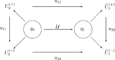
  Figure 1: Diagram showing the connections between the Dirac system, its transformed, and the associated SUSY Schrödinger equations.

• The second possibility is to split the Dirac equation into two Schrödinger equations with potentials $U_{0}^{\pm}$, and then realize a chain of two transformations at the level of the Schrödinger equations, starting with the potential $U_{0}^{+}$; for the first transformation we use $u_{11}$ as the transformation function, and get the potential $U_{0}^{-}$; finally transforming this potential with the help of the transformation function $u_{22}$, we obtain the same potential $\widetilde{U}^{(-)}_{1}$. This path corresponds to $q_{0}\to{U}^{(+)}_{0}\to{U}^{(-)}_{0}\to\widetilde{U}^{(-)}_{1}$ in the diagram.

Other possible path is $q_{0}\to{U}^{(+)}_{0}\to\widetilde{U}^{(+)}_{1}\to\widetilde{U}^{(-)}_{1}$, which is completely equivalent to the previous ones, as it is clear from the preceding discussion. Moreover, as it follows from the scheme of Figure 1, the following proposition holds.

Proposition 4

A Darboux transformation for the Dirac equation with a pseudoscalar potential (121), with transformation function (124), is equivalent to a two-step SUSY transformation for the Schrödinger equation with the potential $U_{0}^{+}$ given by (138) with transformation functions $u_{11}$ and $u_{22}$.

For the case $\lambda_{1}=-m$, $u_{11}=0$, similar calculations give us

$$\widetilde{U}^{(-)}_{1} = q_{0}^{2}+q^{\prime}_{0}=U^{(+)}_{0},$$ (148)

$$\widetilde{U}^{(+)}_{1} = -2(\ln u_{12})^{\prime\prime}+q_{0}^{2}+q^{\prime}_{0}.$$ (149)

We conclude this Section by stressing that Darboux transformation for the Dirac equation induces Darboux transformations for the associated Schrödinger equations.

9 Scalar potentials

9.1 Darboux transformation for a scalar potential

In this Section, let us consider that the initial potential $V_{0}$ has the scalar form

$$V_{0}(x)=p_{0}(x)\sigma_{3}\,,\quad p_{0}=m+S_{0}(x)\,,$$ (150)

where $m$ is the mass of a particle and the function $S_{0}(x)$ is supposed to be known. Note first that if the function $\psi$ is a solution of the Dirac equation with the potential (150) and the energy $E$, then the function $\sigma_{1}\psi$ is also a solution, but with the energy $-E$. In particular, this means that the spectrum of the Dirac equation is symmetric with respect to $E=0$.

In the literature another representation of scalar potentials is frequently used:

$$\widehat{V}_{0}(x)=(m+S_{0}(x))\sigma_{1}\ .$$ (151)

Both representations (150) and (151) are related by a unitary transformation $\widehat{U}$:

$$\widehat{V}_{0}=\widehat{U}^{-1}V_{0}\widehat{U}\,,\qquad\widehat{\psi}=\widehat{U}\psi\ ,$$ (152)

where

$$\widehat{U}=(1+\gamma)/\sqrt{2}\,.$$ (153)

Observe that the scalar potential (151) can be considered as a pseudoscalar potential (121) when the value of the mass is equal to zero. Nevertheless, it has some new properties to be considered below.

The Darboux transformation, in its general form, does not preserve the scalar character of a potential. Therefore, it is necessary to select those transformations such that they will preserve the scalar form of a potential. As it follows from (15)–(18), the transformed potential remains to be scalar if $d_{2}(x)\equiv 0$. From (19) one easily sees that to satisfy this condition it is sufficiently to construct the transformation function ${\mathcal{U}}=(u_{1},u_{2})$ from the spinors $u_{1}=(u_{11},u_{21})^{t}$ and $u_{2}=\sigma_{1}u_{1}$ with eigenvalues $\lambda_{1}=\lambda^{(0)}$ and $\lambda_{2}=-\lambda^{(0)}$, respectively.

In order to look for new properties of the Darboux transformation for the Dirac equation with a scalar potential, it is more convenient to consider the scalar potentials written in the form (151). Under the transformation (153) the potential $V_{0}$ goes into $\widetilde{V}_{0}=(m+S_{0})\sigma_{1}$, and the transformation function ${\mathcal{U}}$ into $\widehat{\mathcal{U}}$, given by

$$\widehat{{\mathcal{U}}}=\left(\begin{array}[]{cc}\widehat{u}_{11}&-\widehat{u}_{11}\\ \widehat{u}_{21}&\widehat{u}_{21}\end{array}\right),$$ (154)

where $\widehat{u}_{11}=u_{11}-u_{21}$, $\widehat{u}_{21}=u_{11}+u_{21}$. For calculating the new potential, we apply (15)–(19), and for getting the transformation operator we use (13), where we have to make the replacement ${\mathcal{U}}\to\widehat{\mathcal{U}}$. The matrix $\widehat{{\mathcal{U}}}_{x}\,\widehat{{\mathcal{U}}}^{-1}$ is now diagonal:

$$\widehat{{\mathcal{U}}}_{x}\,\widehat{{\mathcal{U}}}^{-1}=\left(\begin{array}[]{cc}(\ln\widehat{u}_{11})^{\prime}&0\\[4.30554pt] 0&(\ln\widehat{u}_{21})^{\prime}\end{array}\right).$$ (155)

From Eq. (14) we find that the transformed potential is

$$\widehat{V}_{1}=(m+S_{1})\sigma_{1},$$ (156)

where

$$S_{1}=S_{0}+(\ln\widehat{u}_{21})^{\prime}-(\ln\widehat{u}_{11})^{\prime}.$$ (157)

Solutions of the Dirac equations with the potential (156)–(157) are found by the action of the operator $L=\partial_{x}-\widehat{\mathcal{U}}_{x}\,\widehat{\mathcal{U}}^{-1}$ on solutions of the initial equation:

$$\widehat{\varphi}=L\widehat{\psi}=\left(\begin{array}[]{c}\widehat{\psi}^{\prime}_{1}-(\ln\widehat{u}_{11})^{\prime}\widehat{\psi}_{1}\\[4.30554pt] \widehat{\psi}^{\prime}_{2}-(\ln\widehat{u}_{21})^{\prime}\widehat{\psi}_{2}\end{array}\right).$$ (158)

Remark that if in the positive part of the spectrum of the initial Hamiltonian there exists a ground state level $E=E_{0}$ with wave function $\psi_{0}(x)$, then in the negative part of it there exists a highest energy level $E=-E_{0}$ with wave function $\sigma_{1}\psi_{0}(x)$. The choice of the spinors $u_{1}=\psi_{0}$ and $u_{2}=\sigma_{1}\psi_{0}$ generates a potential $V_{1}$ with the same spectrum as $V_{0}$, except for the levels $\pm E_{0}$.

The use of formula (154) gives us the matrix solution of the transformed Dirac equation with the matrix eigenvalue $\Lambda$

$$\widehat{\mathcal{V}}=(\widehat{{\mathcal{U}}}^{+})^{-1}=\frac{1}{2}\left(\begin{array}[]{cc}(\widehat{u}_{11}^{*})^{-1}&-(\widehat{u}_{11}^{*})^{-1}\\[4.30554pt] (\widehat{u}_{21}^{*})^{-1}&(\widehat{u}_{21}^{*})^{-1}\end{array}\right)\equiv(\widehat{v}_{1},\widehat{v}_{2})$$ (159)

We observe here that the spinors $\widehat{v}_{1}$ and $\widehat{v}_{2}$ are either square integrable or non-integrable simultaneously. In the first case the levels $E=\pm\lambda^{(0)}$ appear in the spectrum of $h_{1}$. Hence, the Darboux transformation may create the energy levels only by pairs symmetrically disposed with respect to $E=0$. This agrees with the fact that it produces a scalar potential which may have only a symmetrical spectrum.

9.2 Interrelation with the Schrödinger equation

It is well-known (see e.g. [33]) that the Dirac system with the scalar potential (151) may be reduced to the following supersymmetric pair of the Schrödinger equations:

$$\begin{array}[]{lcr}-\widehat{\psi}^{\prime\prime}_{1}+U^{(+)}\widehat{\psi}_{1}&=&\varepsilon\widehat{\psi}_{1}\,,\\[4.30554pt] -\widehat{\psi}^{\prime\prime}_{2}+U^{(-)}\widehat{\psi}_{2}&=&\varepsilon\widehat{\psi}_{2}\,.\end{array}$$ (160)

Since the transformed Dirac system also corresponds to a scalar potential, it may be associated with a couple of similar equations

$$\begin{array}[]{lcr}-\widehat{\varphi}^{\prime\prime}_{1}+U^{(+)}_{1}\widehat{\varphi}_{1}&=&\varepsilon_{1}\widehat{\varphi}_{1}\,,\\[4.30554pt] -\widehat{\varphi}^{\prime\prime}_{2}+U^{(-)}_{1}\widehat{\varphi}_{2}&=&\varepsilon_{1}\widehat{\varphi}_{2}\,,\end{array}$$ (161)

where

$$U^{(\pm)}_{1}=(m+S_{1})^{2}\pm S^{\prime}_{1}.$$ (162)

Taking into account the equation for $S_{1}$ (157), after some algebra we get from (162) the potentials $U^{(\pm)}_{1}$

$$U^{(+)}_{1} = (m+S_{0})^{2}+S_{0}^{\prime}-2(\ln\widehat{u}_{11})^{\prime\prime}\,,$$ (163)

$$U^{(-)}_{1} = (m+S_{0})^{2}-S_{0}^{\prime}-2(\ln\widehat{u}_{21})^{\prime\prime}\,.$$ (164)

Hence, we also conclude that the potentials $U^{(\pm)}_{1}$ are SUSY partners of the potentials $U^{(\pm)}_{0}$, and Darboux transformation for the Dirac equation induces Darboux transformations of corresponding supersymmetric pair of initial Schrödinger equations.

10 Illustrative examples

In this Section we will show how the technique we have developed for Dirac systems is applied to some interesting examples of pseudoscalar and scalar potentials, as well as to spherically symmetric potentials.

10.1 Pseudoscalar potentials

First, we will analyse some examples of Darboux transformation applied to transparent potentials, and also to the relativistic harmonic oscillator.

10.1.1 Transparent potentials

In this paper we do not analyse the changes in transmission and reflection coefficients produced by Darboux transformations. Nevertheless, we can easily notice that if the initial potential is transparent, i.e., if it produces the zero reflection coefficient for an incident particle, or if the potential does not change the asymptotic form of a continuous spectrum eigenfunction, then the transformed potential keeps this property unchanged. In particular, this means that starting with the free particle Dirac equation we shall get only transparent potentials. Hence, in this Section let us consider the potential

$$V_{0}=m\sigma_{3},$$ (165)

which is a particular case of (121) with $q_{0}=0$.

Example 1

Let us take as transformation function the following matrix

$${\mathcal{U}}=\left(\begin{array}[]{cc}1&\frac{k}{\varepsilon-m}\ \sinh kx\\[4.30554pt] 0&\cosh kx\end{array}\right)\,,\quad k=\sqrt{m^{2}-\varepsilon^{2}}\,.$$ (166)

It corresponds to $\lambda_{1}=m$, $\lambda_{2}=\varepsilon<m$. The transformed potential is obtained by Eqs. (127) and (128), that generate the well-known one-soliton potential (see e.g. [34, 35]):

$$V_{1}=-\varepsilon\sigma_{3}+k\tanh kx\,\sigma_{1}\ .$$ (167)

From Eq. (166) we find the matrix solution of the transformed Dirac equation for the particular value $E=\Lambda=\mbox{diag}(m,\varepsilon)$:

$${\mathcal{V}}=({\mathcal{U}}^{+})^{-1}=\left(\begin{array}[]{cc}1&0\\[4.30554pt] -\frac{k}{\varepsilon-m}\,\tanh kx&\mbox{sech\,}kx\end{array}\right)\,.$$ (168)

We conclude from (168) that the potential (167) has one discrete level at $E=\varepsilon$. The solutions of the Dirac equation with the potential (167) at $E\neq\varepsilon,m$ may be found by applying the operator $L$ to solutions $\psi$ of the free particle equation:

$${\varphi}=L\psi=\psi_{x}-{\mathcal{U}}_{x}\,{\mathcal{U}}^{-1}\psi\,.$$ (169)

The potential (167) may be considered as the initial potential for the next transformation step. To carry it out, we need a spinor solution of the Dirac equation with either upper or lower component equal to zero. If we take as a solution of the free particle Dirac equation

$$\psi_{1}=\left(\begin{array}[]{c}-\frac{k}{\varepsilon+m}\ \sinh kx\\[4.30554pt] \cosh kx\end{array}\right)$$ (170)

then, from (169) we find the following spinor solution of the Dirac equation for the potential (167):

$${\varphi}_{1}=\left(\begin{array}[]{c}-2\varepsilon\cosh kx\\[4.30554pt] 0\end{array}\right)$$ (171)

corresponding to the eigenvalue $\lambda_{1}=-\varepsilon.$ Another solution of the Dirac equation for this potential (167) may be found with the function

$$\psi_{2}=\left(\begin{array}[]{c}-\frac{k_{1}}{\varepsilon_{1}-m}\ e^{-k_{1}x}\\[4.30554pt] e^{-k_{1}x}\end{array}\right)$$ (172)

in (169), which gives us

$${\varphi}_{2}=\left(\begin{array}[]{c}(\varepsilon-\varepsilon_{1})e^{-k_{1}x}\\[4.30554pt] (k_{1}+k\tanh kx)e^{-k_{1}x}\end{array}\right),\quad k_{1}=\sqrt{m^{2}-\varepsilon_{1}^{2}}.$$ (173)

This spinor has the eigenvalue $\lambda_{2}=\varepsilon_{1}$. From the spinors $u_{1}=\varphi_{1}$ and $u_{2}=\varphi_{2}$ we construct the matrix solution for the potential (167), ${\mathcal{U}}=(u_{1},u_{2})$, with the matrix eigenvalue $\Lambda=\mbox{diag}(-\varepsilon,\varepsilon_{1})$.

Example 2

When the above matrix solution ${\mathcal{U}}$ is taken as the transformation function for the second transformation step, it produces a two-soliton potential of the form:

$$V_{2}=-\varepsilon_{1}\sigma_{3}+\left(\frac{k^{2}-k_{1}^{2}}{k_{1}+k\tanh kx}-k\tanh kx\right)\sigma_{1}\ .$$ (174)

The choice $k_{1}>k>0$ assures the regular behaviour of this potential $V_{2}$, which keeps the discrete level $E=\varepsilon$ unchanged and has an additional level at $E=-\varepsilon$. The last statement can be easily seen from the matrix solution for the potential (174) with matrix eigenvalue $\Lambda=\mbox{diag}(-\varepsilon,\varepsilon_{1})$:

$${\mathcal{V}}=({\mathcal{U}}^{+})^{-1}=\left(\begin{array}[]{cc}\frac{1}{2\varepsilon\cosh kx}&0\\[8.61108pt] \frac{\varepsilon-\varepsilon_{1}}{2\varepsilon\cosh kx(k_{1}+k\tanh kx)}&\frac{-e^{k_{1}x}}{k_{1}+k\tanh kx}\end{array}\right).$$

The first column of this matrix is a square integrable spinor with eigenvalue $E=-\varepsilon$.

Example 3

In (169) let us choose now

$$\psi_{2}=\left(\begin{array}[]{c}\frac{k_{1}}{\varepsilon_{1}-m}\ \cosh k_{1}x\\[4.30554pt] \sinh k_{1}x\end{array}\right),\qquad k_{1}=\sqrt{m^{2}-\varepsilon_{1}^{2}}\,.$$ (175)

This gives us

$$\varphi_{2}=\left(\begin{array}[]{c}(\varepsilon-\varepsilon_{1})\sinh k_{1}x\\[4.30554pt] k_{1}\cosh k_{1}x-k\tanh kx\ \sinh k_{1}x\end{array}\right)\,,\quad k=\sqrt{m^{2}-\varepsilon^{2}}\,.$$ (176)

The use of this spinor as the second component of the transformation function, $u_{2}=\varphi_{2}$, together with the previously found $u_{1}$ as the first component, ${\mathcal{U}}=(u_{1},u_{2})$, produces the following three-soliton potential:

$$V_{2}=-\varepsilon_{1}\sigma_{3}+\left(\frac{k_{1}^{2}-k^{2}}{k_{1}\coth k_{1}x-k\tanh kx}-k\tanh kx\right)\sigma_{1}\ ,$$ (177)

which is regular provided $k_{1}>k>0$, and has three discrete levels: $E=\pm\varepsilon$ and $E=\varepsilon_{1}$.

It is important to stress that similar potentials have been found recently by other means [34]. In contradistinction to these authors, we are able to indicate precisely the position of the discrete levels. Moreover, corresponding wave functions are easily obtained from columns of the matrix-function $({\mathcal{U}}^{+})^{-1}$ In the next example we give more general transparent potential with three discrete levels.

Example 4

We can take the following spinor as a solution of the free particle equation in order to get a solution of the Dirac equation with the one-soliton potential, which is:

$$\psi_{2}=\left(\begin{array}[]{c}\frac{k_{1}}{\varepsilon_{1}-m}(\sinh k_{1}x+B\cosh k_{1}x)\\[4.30554pt] (\cosh k_{1}x+B\sinh k_{1}x)\end{array}\right),$$ (178)

where $B$ is an arbitrary constant. From (169), we obtain

$$\varphi_{2}=\left(\begin{array}[]{c}(\varepsilon-\varepsilon_{1})Q(x)\\[4.30554pt] k_{1}(\sinh k_{1}x+B\cosh k_{1}x)-kQ(x)\tanh kx)\end{array}\right),$$ (179)

where $Q(x)=\cosh k_{1}x+B\sinh k_{1}x$. When $\varphi_{2}$ is used as the spinor $u_{2}$ for the second transformation step, it produces the potential

$$V_{2} = -\varepsilon_{1}\sigma_{3}$$

$$+\left(\frac{(k_{1}^{2}-k^{2})(1+B\tanh k_{1}x)}{k_{1}(\tanh k_{1}x+B)-k\tanh kx(1+B\tanh k_{1}x)}-k\tanh kx\right)\sigma_{1}\,.$$

It is not difficult to prove that it is regular provided $k_{1}>k>0$ and $B>1$, and also that it has three discrete levels: $E=\pm\varepsilon$ and $E=\varepsilon_{1}$. A typical behavior of this potential is shown in Figure 2, where the term between parentheses in Eq. (4) is plotted. One can notice that closer is the parameter $B$ to the value $1$, wider is the potential barrier.

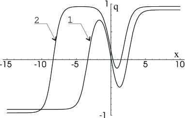
Figure 2: Three-level transparent pseudoscalar potentials with $m=1$ and $\varepsilon=0.5$. Curve 1 is obtained for $B=1.5$ and $\varepsilon=0.45$ Curve 2 is obtained for $B=1.000005$ and $\varepsilon=0.3$.

A potential of this type is not known in the available literature.

To finish this subsection, we would like to remark that our method can produce transparent potentials of a more general form, which are a superposition of scalar and pseudoscalar potentials. We illustrate this fact in he next example

Example 5

As a final case of transparent potentials, let us consider as transformation function the following matrix solution of the free particle Dirac equation:

$${\mathcal{U}}=\left(\begin{array}[]{cc}-\frac{k}{\varepsilon+m}\ \sinh kx&\frac{k}{\varepsilon-m}\ e^{kx}\\[4.30554pt] \cosh kx&e^{kx}\end{array}\right),\ \lambda_{1}=-\varepsilon,\ \lambda_{2}=\varepsilon,\ k=\sqrt{m^{2}-\varepsilon^{2}}.$$ (181)

It generates a completely new potential of the form

$$V_{1}=\left[m-\frac{2k^{2}}{\varepsilon{e^{2kx}}^{\vphantom{j}}+m}\right]\sigma_{3}+2k\varepsilon\,\frac{\sinh kx-\cosh kx}{\varepsilon e^{kx}+m{e^{-kx}}^{\vphantom{j}}}\ \sigma_{1}\,.$$ (182)

From the analysis of the function

$$({\mathcal{U}}^{+})^{-1}=\left(\begin{array}[]{cc}\displaystyle\frac{k}{\varepsilon e^{kx}+m{e^{-kx}}^{\vphantom{j}}}&\displaystyle\frac{-k\cosh kx}{\varepsilon{e^{2kx}}^{\vphantom{j}}+m}\\[8.61108pt] \displaystyle\frac{m+\varepsilon}{\varepsilon e^{kx}+m{e^{-kx}}^{\vphantom{j}}}&\displaystyle\frac{(\varepsilon-m)\sinh kx}{\varepsilon{e^{2kx}}^{\vphantom{j}}+m}\end{array}\right)$$

we conclude that $V_{1}$ has one discrete level $E=-\varepsilon$.

10.1.2 Darboux transformation for the Dirac oscillator

As it is well known, in the literature there are several possible candidates to be considered as the relativistic Dirac oscillator. We choose the one which is described by the Hamiltonian [36]

$$h_{0}=\gamma\partial_{x}+m\sigma_{3}+\frac{x}{2}\sigma_{1}\,.$$ (183)

Its discrete spectrum consists of a positive series

$$E^{(+)}_{n}=(m^{2}+n)^{1/2},\qquad n=1,2,\ldots$$ (184)

and a negative series

$$E^{(-)}_{n}=-(m^{2}+n)^{1/2},\qquad n=0,1,\ldots.$$ (185)

We will use this model to illustrate the aplications of the Darboux transformation for the Dirac equation in three examples.

Example 6

We will use the spinors

$$u_{1}=\left(\begin{array}[]{c}e^{x^{2}/2}\\[4.30554pt] 0\end{array}\right),$$ (186)

and

$$u_{2}=\left(\begin{array}[]{c}-\frac{i}{\varepsilon_{n}-m}\ e^{x^{2}/4}\ \mbox{He}_{n}(ix)\\[8.61108pt] e^{x^{2}/4}\ \mbox{He}_{n-1}(ix)\end{array}\right),$$ (187)

for constructing the transformation function ${\mathcal{U}}=(u_{1},u_{2})$. The spinor (186) is a solution of the Dirac equation with the potential (183) for $\lambda_{1}=m$; the same is true for the spinor (187) with eigenvalue $\lambda_{2}=\varepsilon_{n}=(m^{2}-n)^{1/2}$. Here

$$\mbox{He}_{n}(z)=2^{-n/2}H_{n}(z/\sqrt{2})\,,$$ (188)

where $H_{n}(z)$ are Hermite polynomials. Using the formulas (127) and (128) we obtain the transformed potential

$$V_{1}=-\varepsilon_{n}\sigma_{3}+\left(\frac{x}{2}+(n-1)\ \frac{K_{n-2}(x)}{K_{n-1}(x)}\right)\sigma_{1}\,,$$ (189)

where $K_{n}(x)=(-i)^{n}\,\mbox{He}_{n}(ix)$. Observe that the functions $K_{n}(x)$ are real and nodeless for even values of $n$; for odd values of $n$ they have only one node at $x=0$ [29]. Therefore, the potentials (189) are real and regular when $n$ takes odd values. The analysis of the function $({{\mathcal{U}}^{+}})^{-1}$ shows that this potential has two additional discrete levels $E=m$ and $E=\varepsilon_{n}$ with respect to the initial harmonic oscillator potential (183).

Example 7

Let us keep the spinor $u_{2}$ as in the previous example and let us take $u_{1}=(0,\ e^{-x^{2}/2})^{t}$, which corresponds to $\lambda_{1}=-m$. Using the same procedure of the previous example, we get the potential

$$V_{1}=\varepsilon_{n}\,\sigma_{3}-\left(\frac{x}{2}+n\ \frac{K_{n-1}(x)}{K_{n}(x)}\right)\sigma_{1}\,.$$ (190)

In contrast to the previous example, $\lambda_{1}$ belongs now to the discrete spectrum of the initial potential. Therefore, the level $E=-m$ is deleted from the spectrum of the Hamiltonian (183) and the new level $E=\varepsilon_{n}$ is added. The potential (190) is everywhere regular for even values of $n$.

Example 8

Finally, let us take now the spinor $u_{1}$ as in Example 1 and choose the spinor $u_{2}$ as follows:

$$u_{2}=\left(\begin{array}[]{c}\frac{1}{\lambda_{2}-m}\ (x\,Q(x)\ e^{x^{2}/4}+e^{-x^{2}/4})\\[4.30554pt] Q(x)\ e^{x^{2}/4}\end{array}\right),$$ (191)

which corresponds to $\lambda_{2}=(m^{2}-1)^{1/2}$. Here, $Q(x)=\sqrt{\pi/2}\,(B+\mbox{erf}(x/\sqrt{2}))$, with $|B|>1$. We get for the transformed potential

$$V_{1}=-\lambda_{2}\sigma_{3}+\left(\frac{x}{2}+e^{-x^{2}/2}\,Q^{-1}(x)\right)\sigma_{1}\,.$$ (192)

A simple analysis shows that this potential has two additional discrete levels $E=m$ and $E=(m^{2}-1)^{1/2}$ with respect to the initial potential (183). Two typical representatives of this potential are displayed in Figure 3, where the term between parentheses in Eq. (192) is plotted. It is clearly seen that closer is the parameter $B$ to the value $1$, larger is the perturbation of the initial potential.

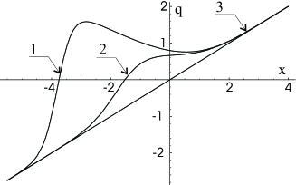
Figure 3: Harmonic oscillator potential $q_{0}(x)=x/2$ (curve 3) with $m=1$, and two of its Darboux transformed partners $q_{1}(x)$. Curve 1 is obtained for $B=1.0002$, and curve 2 for $B=1.2$.

10.2 Scalar potentials

In this subsection we will analise some scalar potentials of the form (151)

$$\widehat{V}_{0}(x)=p_{0}(x)\sigma_{1}=(m+S_{0}(x))\sigma_{1}\,.$$

In the first instance, we will consider the simplest case, corresponding to $S_{0}(x)\equiv 0$.

10.2.1 Transparent potentials

Example 9

The spinor

$$\widehat{u}_{1}=\left(\begin{array}[]{c}e^{kx}+e^{-kx}\\[4.30554pt] \frac{m-k}{\lambda}\ e^{kx}+\frac{m+k}{\lambda}\ e^{-kx}\end{array}\right),\qquad k=\sqrt{m^{2}-\lambda^{2}},$$ (193)

is a solution of the Dirac equation with potential $\widehat{V}_{0}=m\sigma_{1}$ for $E=\lambda<m$. Choosing the transformation function in the form $\widehat{\mathcal{U}}=(\widehat{u}_{1},\widehat{u}_{2})$, $\widehat{u}_{2}=-\sigma_{3}\widehat{u}_{1}$, and using Eq. (157), we get the transformed potential

$$S_{1}=-\frac{2k^{2}}{m+\lambda\cosh(2kx+2\alpha)},$$ (194)

where $e^{2\alpha}=\sqrt{(m-k)/(m+k)}$. This is a transparent potential, which has been previously found in [33]. It is easy to see that the two spinors coming from the matrix $(\widehat{{\mathcal{U}}}^{+})^{-1}$ are square integrable. This means that the potential (194) has two discrete levels: $E=\pm\lambda$.

Example 10

Consider now the spinor

$$\widehat{v}_{1}=\left(\begin{array}[]{c}\sinh k_{1}x\\[4.30554pt] \sinh(k_{1}x+2\alpha_{1})\end{array}\right),\quad k_{1}=\sqrt{m^{2}-\lambda_{1}^{2}},\ \ e^{2\alpha_{1}}=\sqrt{\frac{m-k_{1}}{m+k_{1}}},$$ (195)

satisfying the free Dirac equation for $E=\lambda_{1}<m$. After acting on it with the transformation operator of the Example 1, we get the spinor

$$\widehat{w}_{1}=\left(\begin{array}[]{c}k_{1}\cosh k_{1}x-k\tanh kx\,\sinh k_{1}x\\[4.30554pt] k_{1}\cosh(k_{1}x+2\alpha_{1})-k\tanh kx\,\sinh(k_{1}x+2\alpha_{1})\end{array}\right),$$ (196)

which is a solution of the Dirac equation with the potential (194). If we choose the spinors $\widehat{w}_{1}$ and $\widehat{w}_{2}=-\sigma_{3}\widehat{w}_{1}$ for the next transformation step, we obtain a two-step potential

$$S_{2} = \frac{k_{1}^{2}-k^{2}}{k_{1}\coth(k_{1}x+2\alpha_{1})-k\tanh(kx+2\alpha)}$$ (197)

$$-\frac{k_{1}^{2}-k^{2}}{k_{1}\coth k_{1}x-k\tanh kx}\,.$$

For $0<k<k_{1}<m$ this is a regular transparent potential with four discrete levels $E=\pm\lambda$ and $E=\pm\lambda_{1}$. Figure 4 shows the typical shape of such potentials. From this figure it is clearly seen that closer are the discrete levels of the potential, more distant from each other are the two potential wells.

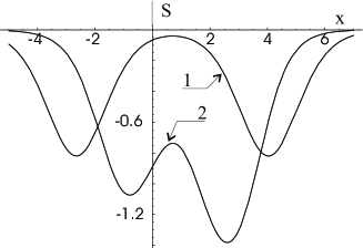
Figure 4: Four-level scalar potentials with $m=1$ and $\lambda=0.6$. Curve 1 is obtained for $\lambda_{1}=0.58$, and curve 2 for $\lambda_{1}=0.2$.

10.2.2 Scalar Coulomb potential

We will analise now radial potentials of the form

$$\widehat{V}_{0}=\left(m-\frac{\alpha}{r}\right)\sigma_{1},\qquad\alpha>0,$$ (198)

which find applications in modelling inter-quark interactions [37]. In this case, the discrete spectrum of the Dirac Hamiltonian consists of a positive and a negative series [38]

$$E_{n}=\pm m\ \sqrt{1-\frac{\alpha^{2}}{(n+\alpha)^{2}}},\quad n=1,2,\ldots,$$ (199)

plus the zero energy level $E=0$ [39]. The eigenfunctions of the discrete spectrum (not normalized here) have the form

$$\widetilde{\psi}_{n}=\left(\begin{array}[]{c}-\frac{E_{n}\,(n-1)!}{\varepsilon_{n}(2\alpha+1)_{n}}\ e^{-x}\ x^{\alpha+1}\ L^{2\alpha+1}_{n-1}(2x)\\[8.61108pt] \frac{n!}{(2\alpha)_{n}}\ e^{-x}\ x^{\alpha}\ L^{2\alpha-1}_{n}(2x)\end{array}\right),$$ (200)

where $\varepsilon_{n}=\sqrt{m^{2}-{E_{n}^{2}}^{\vphantom{k}}}$ and $x=\varepsilon_{n}r$, $n=1,2,\ldots$ .

Example 11

In order to apply the two-step Darboux transformation described in Section 7, let us take the spinors $\widehat{\mathcal{U}}=(\widehat{u}_{1},\widehat{u}_{2})$, with $\widehat{u}_{1}=\widehat{\psi}_{k}$ and $\widehat{u}_{2}=-\sigma_{3}\widehat{\psi}_{k}$, and $\widehat{\mathcal{V}}=(\widehat{v}_{1},\widehat{v}_{2})$, with $\widehat{v}_{1}=\widehat{\psi}_{k+1}$ and $\widehat{v}_{2}=-\sigma_{3}\widehat{\psi}_{k+1}$. For the transformed potential we obtain

$$\widehat{V}^{(k)}_{2}(x)=(m+S^{(k)}_{2}(x))\sigma_{1},\ S^{(k)}_{2}=-\frac{\alpha}{r}+(\ln{Q_{2}(r)})^{\prime}-(\ln{Q_{1}(r)})^{\prime},$$ (201)

where

$$Q_{1}(r) = \frac{kL^{2\alpha+1}_{k}(2\varepsilon_{k+1}r)L^{2\alpha-1}_{k}(2\varepsilon_{k}r)}{2\alpha+k+1}-\frac{(k+1)L^{2\alpha+1}_{k-1}(2\varepsilon_{k}r)L^{2\alpha-1}_{k+1}(2\varepsilon_{k+1}r)}{2\alpha+k},$$

$$Q_{2}(r) = \frac{L^{2\alpha+1}_{k}(2\varepsilon_{k+1}r)L^{2\alpha-1}_{k}(2\varepsilon_{k}r)}{(\alpha+k+1)^{2}}-\frac{L^{2\alpha+1}_{k-1}(2\varepsilon_{k}r)L^{2\alpha-1}_{k+1}(2\varepsilon_{k+1}r)}{(\alpha+k)^{2}}.$$

The spectrum of $\widehat{V}^{(k)}_{2}(x)$ differs from the spectrum of the initial Coulomb potential by the absence of the levels $E=E_{k}$ and $E=E_{k+1}$. We would like to remark that after the first transformation, either with the spinor $\widehat{u}_{1}$ or with $\widehat{u}_{2}$, we get potentials with singularities, but the second transformation removes all singularities and the potential (201) is regular for $r>0$. The simplest particular case corresponds to $k=1$:

$$S^{(1)}_{2}=-\frac{\alpha+2}{r}+\frac{2m(2mr-2\alpha-3)}{2m^{2}r^{2}-2m(2\alpha+3)r+(\alpha+2)(2\alpha+3)}\,.$$ (202)

The behavior of the potential (201) at $k=4$, $m=1$ and $a=1$ is shown in Figure 5.

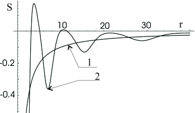
Figure 5: Scalar Coulomb potential $S_{0}(r)$ (curve 1) and its Darboux transformed partner $S_{2}^{(4)}(r)$ (curve 2).

10.3 Spherically symmetric potentials

The first important detail to be taken into account is that the usual (3+1)-dimensional Dirac equation with a spherically symmetric potential is included in our developments. Indeed, using the standard technique of separation of angular variables (see e.g. [40]), we get the following radial equation coupled to scalar $W_{s}(r)$, pseudoscalar $W_{p}(r)$ and vector $W_{v}(r)$ potentials:

$$\left\{\frac{d}{dr}-\left[\frac{k}{r}+W_{P}\right]\sigma_{3}+[m+W_{s}]\sigma_{1}+i[E-W_{v}]\sigma_{2}\right\}\psi(r)=0,$$ (203)

where $r$ is the radial variable, $m$ is the mass of the particle, and $E$ its energy, while $k=\pm 1,\pm 2\ldots$ is related to the total angular momentum. Eq. (203) can be also written as

$$\left\{i\sigma_{2}\frac{d}{dr}+\left[\frac{k}{r}+W_{P}\right]\sigma_{1}+\left[m+W_{s}\right]\sigma_{3}-\left[E-W_{v}\right]\right\}\psi(r)=0\,,$$ (204)

which if $W_{v}(r)\equiv 0$ coincides with $h_{0}\psi(r)=E\psi(r)$, $h_{0}=\gamma\partial_{r}+V_{0}(r)$, being $V_{0}(r)$ given in the canonical form (21) with

$$p_{0}(r)=m+W_{s}(r)\,,\quad q_{0}(r)=W_{p}(r)+\frac{k}{r}\,.$$ (205)

Let us start with an unphysical potential, corresponding to $p_{0}(r)=q_{0}(r)=0$ and $k=0$, i.e. $V_{0}=m\sigma_{3}$. The associated Dirac Hamiltonian will be denoted by $h_{0}$ and its eigenfunctions by $\psi(E)$, where we omit the evident dependence on the variable $r$ and we stress only the dependence on the eigenvalue $E$. We will show that, starting with $h_{0}$, one can obtain physically meaningful potentials with $k\neq 0$. For this purpose, we shall use the eigenfunctions of $h_{0}$ with $E=\pm m$:

$$\psi(m)=\left(\begin{array}[]{c}1\\ 0\end{array}\right)\,, \widetilde{\psi}(m)=\left(\begin{array}[]{c}-2mr\\ 1\end{array}\right)\,.$$ (210)

$$\psi(-m)=\left(\begin{array}[]{c}0\\ 1\end{array}\right)\,, \widetilde{\psi}(-m)=\left(\begin{array}[]{c}1\\ -2mr\end{array}\right)\,.$$ (215)

Other eigenfunctions will be also used for producing new nontrivial potentials

$$\psi(\lambda)=\left(\begin{array}[]{c}\cosh kr\\[4.30554pt] -\frac{k}{\lambda+m}\ \sinh kr\end{array}\right)\,,$$ (216)

$$\widetilde{\psi}(\lambda)=e^{-kr}\left(\begin{array}[]{c}1\\[4.30554pt] \frac{k}{\lambda+m}\end{array}\right)\,,\quad k^{2}=m^{2}-\lambda^{2}>0\,.$$ (217)

Example 12

Let us take the spinors $u_{1}$ and $u_{2}$ from which the transformation function ${\mathcal{U}}$ is constructed as follows: $u_{1}=\psi(m)$, $u_{2}=\widetilde{\psi}(-m)$. After a very simple algebra, we obtain the potential

$$V_{1}=m\sigma_{3}+\frac{1}{r}\sigma_{1},$$

which is just the free particle Dirac Hamiltonian with $k=1$. It is not difficult to see that the choice $u_{1}=\psi(-m)$, $u_{2}=\widetilde{\psi}(m)$ gives the same Hamiltonian, but with $k=-1$.

Now, all solutions of the Dirac equation with the potential $V_{1}=m\sigma_{3}+\frac{1}{r}\sigma_{1}$ can be found either by applying the transformation operator (13) to solutions of the same equation with $V_{0}=m\sigma_{3}$, or by applying formulas (34) and (30)–(32). Two solutions with $E=m$ are

$$\varphi(m)=\left(\begin{array}[]{c}1\\ \frac{1}{2mr}\end{array}\right)\,,\quad\widetilde{\varphi}(m)=\left(\begin{array}[]{c}r\\ 0\end{array}\right).$$ (218)

For $E=-m$ one gets

$$\varphi(-m)=\left(\begin{array}[]{c}0\\ {1}/{r}\end{array}\right)\,,\quad\widetilde{\varphi}(-m)=\left(\begin{array}[]{c}-3r\\ 2mr^{2}\end{array}\right).$$ (219)

The solutions with $E\neq\pm m$ have the form

$$\varphi(\lambda)=L\psi(\lambda)=k\left(\begin{array}[]{c}-\sinh kr\\[4.30554pt] \frac{-k}{\lambda-m}\ \cosh kr+\frac{1}{(\lambda-m)r}\ \sinh kr\end{array}\right)\,,$$ (222)

$$\widetilde{\varphi}(\lambda)=L\widetilde{\psi}(\lambda)=ke^{-kr}\left(\begin{array}[]{c}1\\ \frac{k}{\lambda}+\frac{1}{\lambda r}\end{array}\right)\,.$$ (225)

If we take now the spinors $u_{1}=\widetilde{\varphi}(m)$ and $u_{2}=\widetilde{\varphi}(-m)$ for constructing the transformation function ${\mathcal{U}}$ of the second transformation step, we find after some algebra the free Dirac Hamiltonian with $k=2$.

In the next example we illustrate how the use of a spinor having one of its components equal to zero inside the transformation function produces a pseudoscalar potential.

Example 13

The spinors $u_{1}=\widetilde{\varphi}(m)$ and $u_{2}=\widetilde{\varphi}(\lambda)$ give the simplest pseudoscalar potential with the mass equal to $-\lambda$

$$q_{2}(r)=-\frac{1}{r}-\frac{k^{2}r}{1+kr}\,,$$ (226)

whereas the choice $u_{2}=\varphi(\lambda)$ corresponds to

$$q_{2}(r)=\frac{2}{r}-\frac{3kr\cosh kr-(3+k^{2}r^{2})\sinh kr}{r(kr\cosh kr-\sinh kr)}\,.$$ (227)

Another possibility to get a pseudoscalar potential is by choosing $u_{1}=\widetilde{\varphi}(\lambda)$ and $u_{2}=\widetilde{\varphi}(-\lambda)$. By this means we get the potential corresponding to the same mass $m$ and

$$q_{2}(r)=\frac{2}{r}-\frac{k\cosh kr+k^{2}r^{2}\mbox{cosech}\,kr-2\sinh kr}{r(kr\cosh kr-\sinh kr)}\,.$$ (228)

In the final example we are going to consider in this paper, a superposition of scalar and pseudoscalar potentials is shown.

Example 14

We use here a linear combination of two spinors with eigenvalue $m$: $u_{1}=c\varphi(m)+\widetilde{\varphi}(m)$ ($c$ is a constant) and $u_{2}=\widetilde{\varphi}(-m)$. Then, we obtain a potential with

$$p_{2}(r) = 2m-\frac{16(cm^{3}r^{2}+2m^{4}r^{3})}{3c+4cm^{2}r^{2}+8m^{3}r^{3}}\,,$$ (229)

$$q_{2}(r) = -\frac{1}{r}+\frac{8m^{2}r(2c+3mr)}{8m^{3}r^{3}+c(3+4m^{2}r^{2})}\,.$$ (230)

This potential is regular provided $c>0$.

Finally, we choose a transformation function composed by following spinors: $u_{1}=\varphi(m)$ and $u_{2}=\varphi(\lambda)$, and we produce another exactly solvable potential corresponding to

$$p_{2}(r) = -\frac{2kmr\lambda\cosh kr+(k^{2}+m(m-\lambda))\sinh kr}{2kmr\cosh kr+(\lambda-m)\sinh kr}\,,$$ (231)

$$q_{2}(r) = k\ \frac{2kmr\sinh kr-k(m+\lambda)\cosh kr}{2kmr\cosh kr+(\lambda-m)\sinh kr}\,.$$ (232)

The Darboux transformation for a generalized Coulomb interaction is considered in [41].

11 Conclusion and outlook

In this paper only a small part of the properties of differential intertwining (Darboux) operators for the one-dimensional Dirac equation has been considered. We have shown that some properties known for the case of the Schrödinger equation, like factorization of Hamiltonians, one-to-one correspondence between spaces of solutions of equations related with an intertwiner, supersymmetry, and determinant formulas for chains of transformations, also have their counterparts for the case of the Dirac equation. We have shown with numerous examples that this technique is as easily as in the case of the Schrödinger equation. Therefore, we hope that this paper will stimulate further investigations in this field.

To put an end to this paper, we would like to enumerate some subjects that, from our point of view, are worth to be investigated in the future:

1. To get purely scalar spherically symmetric potentials.

2. To find conditions for a chain of transformations to produce regular potentials.

3. To find interrelation between differential and integral transformation operators.

4. To find transformation of scattering data such as transmission and reflection coefficients, phase shifts.

5. To consider transformations of periodical potentials.

6. To apply this technique for describing the scattering of particles at high energies.

References

- [1] D. J. Fernández C., V. Hussin, and B. Mielnik, Phys. Lett. A 244 (1998), 309.
- [2] J. Negro, L. M. Nieto, and O. Rosas-Ortiz, J. Math. Phys. 41 (2000), 7964.
- [3] D. J. Fernández C., J. Negro, and L. M. Nieto, Phys. Lett. A 275 (2000), 338.
- [4] B. F. Samsonov, Phys. Lett. A 263 (1999), 274.
- [5] J. C. Cariñena, A. Ramos, and D. J. Fernández C., Ann. Phys. NY 292 (2001), 42.
- [6] D. J. Fernández C., B. Mielnik, O Rosas-Ortiz, and B. F. Samsonov, J. Phys. A 35 (2002), 4279.
- [7] A. A. Andrianov, N. V. Borisov, M. V. Ioffe, and M. I. Eides, Theor. Math. Phys. 61 (1984), 17.
- [8] E. Witten, Nucl. Phys. B 185 (1981), 513; Nucl. Phys. B 202 (1982), 253.
- [9] G. Darboux, “Leçons sur la théorie générale des surfaces et les application géométriques du calcul infinitésimale.” Deuxiéme partie. - Paris, Gautier-Villar et Fils. 1889; Compt. Rend. Acad. Sci. Paris. 94 (1882), 1343; Compt. Rend. Acad. Sci. Paris. 94 (1882), 1456.
- [10] V. Matveev and M. Salle, “Darboux Transformations and Solitons”, New York, Springer, 1991.
- [11] C. V. Sukumar, J. Phys. A 18 (1985), 2937.
- [12] V. P. Berezovoy and A. I. Pashnev, Theor. Math. Phys. 74 (1988), 392.
- [13] D. Baye, Phys. Rev. Lett. 58 (1987), 2738; L. U. Ancarani and D. Baye, Phys. Rev. A46 (1992), 206; D. Baye, Phys. Rev. A 48 (1993), 2040; D. Baye and J. -M. Sparenberg, Phys. Rev. Lett. 73 (1994), 2789; G. Lévai, D. Baye and J. -M. Sparenberg, J. Phys. A 30 (1997), 8257; J. -M. Sparenberg and D. Baye, Phys. Rev. Lett. 79 (1997), 3802; H. Leeb, S. A. Sofianos, J. -M. Sparenberg and D. Baye, Phys. Rev. C 62 (2000), 064003.
- [14] E. Schrödinger, Proc. Roy. Irish. Acad. A. 46 (1940), 9; Proc. Roy. Irish. Acad. A. 47 (1941), 53.
- [15] H. Hull and T. E. Infeld, Phys. Rev. 74 (1948), 905; Phys. Rev. 59 (1941), 737; Rev. Mod. Phys. 53 (1951), 21.
- [16] A. Anderson, Phys. Rev. A 43 (1991), 4602.
- [17] A. A. Stahlhofen, J. Phys. A 27 (1994), 8279.
- [18] M. A. Salle, Theor. Math. Phys. 53 (1982), 1092.
- [19] M. A. Salle, Zapiski Nauchnnih Seminarov LOMI 161 (1987), 72.
- [20] V. B. Daskalov and E. Kh. Khristov, Inv. Probl. 16 (2000), 247.
- [21] P. Prats and J. S. Toll, Phys. Rev. 113 (1959), 363.
- [22] M. B. Levitan and I. S. Sargsian, Introduction to Spectral Theory, American Mathematical Siciety, Providence, Rhode Island, 1975.
- [23] B. F. Samsonov and A.A. Pecheritsin, Rus. Phys. J. 43(1) (2000), 48; Rus. Phys. J. 45(1) (2002), 14; Rus. Phys. J. 45(1) (2002), 74.
- [24] M. M. Crum Quart. J. Math. Ser 2, 6 (1955), 121.
- [25] V. G. Bagrov and B. F. Samsonov, Theor. Math. Phys. 104 (1995), 356.
- [26] V. Smirnov, “Advanced Course of Mathematics”, Vol. 5, Phys.-Math. Publishing State House, Moscow, 1958.
- [27] M. Reed and B. Simon, “Methods of Modern Mathematical Physics. I. Functional Analysis”, Academic, New York, 1972.
- [28] N. Dunford and J. T. Schwartz, “Linear Operators. Part II. Spectral Theory. Self-Adjoint Operators in Hilbert Spaces”, Interscience, New York, 1963.
- [29] V. G. Bagrov and B. F. Samsonov, Phys. Part. Nucl. 28 (1997), 951.
- [30] J. Beckers, N. Debergh and C. Gotti, Helv. Phys. Acta 71 (1998), 214.
- [31] Y. Nogami and F. M. Toyama, Phys. Rev. A 57 (1998), 93.
- [32] B. K. Bagchi, “Supersymmetry in Quantum and Classical Mechanics”, Chapman and Hall, New York, 2001.
- [33] Y. Nogami and F. M. Toyama, Phys. Rev. A 47 (1993), 1708.
- [34] F. M. Toyama and Y. Nogami, Phys. Rev. A 57 (1998), 93.
- [35] B. Thaler, “The Dirac Equation”, Springer, Berlin, 1992.
- [36] Y. Nogami and F. M. Toyama, J. Phys. A 30 (1997), 2585.
- [37] S. Benvegnu, J. Math. Phys. 38 (1997), 556.
- [38] F. Domínguez-Adame, Am. J. Phys. 58 (1990), 886.
- [39] Ho Choon-Lin and V. R. Khalilov, Phys. Rev. D 63 (2000), 027701.
- [40] J. Weidman, “Spectral Theory of Ordinary Differential Operators”, Lect. Notes Math., Vol. 1258, Springer, Berlin, 1987.
- [41] N. Debergh, A. A. Pecheritsin, B. F. Samsonov and B. Van Den Bossche, J. Phys. A 35 (2002), 3279.