Lower Bounds for Local Search by Quantum Arguments

Abstract

The problem of finding a local minimum of a black-box function is central for understanding local search as well as quantum adiabatic algorithms.  For functions on the Boolean hypercube $\left\{0,1\right\}^{n}$, we show a lower bound of $\Omega\left(2^{n/4}/n\right)$ on the number of queries needed by a quantum computer to solve this problem.  More surprisingly, our approach, based on Ambainis’s quantum adversary method, also yields a lower bound of $\Omega\left(2^{n/2}/n^{2}\right)$ on the problem’s classical randomized query complexity.  This improves and simplifies a 1983 result of Aldous.  Finally, in both the randomized and quantum cases, we give the first nontrivial lower bounds for finding local minima on grids of constant dimension $d\geq 3$.

1 Introduction

This paper deals with the following problem.

Local Search. Given an undirected graph $G=\left(V,E\right)$ and a function $f:V\rightarrow\mathbb{N}$, find a local minimum of $\mathit{f}$—that is, a vertex $v$ such that $f\left(v\right)\leq f\left(w\right)$ for all neighbors $w$ of $v$.

We are interested in the number of queries that an algorithm needs to solve this problem, where a query just returns $f\left(v\right)$ given $v$.  We consider deterministic, randomized, and quantum algorithms.  Section 2 motivates the problem theoretically and practically; this section explains our results.

We start with some simple observations.  If $G$ is the complete graph of size $N$, then clearly $\Omega\left(N\right)$ queries are needed to find a local minimum (or $\Omega\left(\sqrt{N}\right)$ with a quantum computer [9]).  At the other extreme, if $G$ is a line of length $N$, then even a deterministic algorithm can find a local minimum in $O\left(\log N\right)$ queries, using binary search: query the middle two vertices, $v$ and $w$.  If $f\left(v\right)\leq f\left(w\right)$, then search the line of length $\left(N-2\right)/2$ connected to $v$; otherwise search the line connected to $w$.  Continue recursively in this manner until a local minimum is found.

So the interesting case is when $G$ is a graph of ‘intermediate’ connectedness: for example, the Boolean hypercube $\left\{0,1\right\}^{n}$, with two vertices adjacent if and only if they have Hamming distance $1$.  For this graph, Llewellyn, Tovey, and Trick [19] showed a $\Omega\left(2^{n}/\sqrt{n}\right)$ lower bound on the number of queries needed by any deterministic algorithm, using a simple adversary argument.  Intuitively, until the set of vertices queried so far comprises a vertex cut (that is, splits the graph into two or more connected components), an adversary is free to return a descending sequence of $f$-values: $f\left(v_{1}\right)=2^{n}$ for the first vertex $v_{1}$ queried by the algorithm, $f\left(v_{2}\right)=2^{n}-1$ for the second vertex queried, and so on.  Moreover, once the set of queried vertices does comprise a cut, the adversary can choose the largest connected component of unqueried vertices, and restrict the problem recursively to that component.  So to lower-bound the deterministic query complexity, it suffices to lower-bound the size of any cut that splits the graph into two reasonably large components.  For the Boolean hypercube, Llewellyn et al. showed that the best one can do is essentially to query all $\Omega\left(2^{n}/\sqrt{n}\right)$ vertices of Hamming weight $n/2$.

Llewellyn et al.’s argument fails completely in the case of randomized algorithms.  By Yao’s minimax principle, what we want here is a fixed distribution $\mathcal{D}$ over functions $f:\left\{0,1\right\}^{n}\rightarrow\mathbb{N}$, such that any deterministic algorithm needs many queries to find a local minimum of $f$, with high probability if $f$ is drawn from $\mathcal{D}$.  Taking $\mathcal{D}$ to be uniform will not do, since a local minimum of a uniform random function is easily found.  However, Aldous [3] had the idea of defining $\mathcal{D}$ via a random walk, as follows.  Choose a vertex $v_{0}\in\left\{0,1\right\}^{n}$ uniformly at random; then perform an unbiased walk $v_{0},v_{1},v_{2},\ldots$ starting from $v_{0}$.  For each vertex $v$, set $f\left(v\right)$ equal to the first hitting time of the walk at $v$—that is, $f\left(v\right)=\min\left\{t:v_{t}=v\right\}$.  Clearly any $f$ produced in this way has a unique local minimum at $v_{0}$, since for all $t>0$, if vertex $v_{t}$ is visited for the first time at step $t$ then $f\left(v_{t}\right)>f\left(v_{t-1}\right)$.  Using sophisticated random walk analysis, Aldous managed to show a lower bound of $2^{n/2-o\left(n\right)}$ on the expected number of queries needed by any randomized algorithm to find $v_{0}$.  (As we will see in Section 3, this lower bound is close to tight.)  Intuitively, since a random walk on the hypercube mixes in $O\left(n\log n\right)$ steps, an algorithm that has not queried a $v$ with $f\left(v\right)<2^{n/2}$ has almost no useful information about where the unique minimum $v_{0}$ is, so its next query will just be a “stab in the dark.”

Aldous’s result leaves several questions about Local Search unanswered.  What if the graph $G$ is a $3$-D cube, on which a random walk does not mix very rapidly?  Can we still lower-bound the randomized query complexity of finding a local minimum?  More generally, what parameters of $G$ make the problem hard or easy?  Also, what is the quantum query complexity of Local Search?

This paper presents a new approach to Local Search, which we believe points the way to a complete understanding of its complexity.  Our approach is based on the quantum adversary method, introduced by Ambainis [5] to prove lower bounds on quantum query complexity.  Surprisingly, our approach yields new and simpler lower bounds for the problem’s classical randomized query complexity, in addition to quantum lower bounds.  Thus, along with recent work by Kerenidis and de Wolf [17] and by Aharonov and Regev [2], this paper illustrates how quantum ideas can help to resolve classical open problems.

Our results are as follows.  For the Boolean hypercube $G=\left\{0,1\right\}^{n}$, we show that any quantum algorithm needs $\Omega\left(2^{n/4}/n\right)$ queries to find a local minimum on $G$, and any randomized algorithm needs $\Omega\left(2^{n/2}/n^{2}\right)$ queries (improving the $2^{n/2-o\left(n\right)}$ lower bound of Aldous [3]).  Our proofs are elementary and do not require random walk analysis.  By comparison, the best known upper bounds are $O\left(2^{n/3}n^{1/6}\right)$ for a quantum algorithm and $O\left(2^{n/2}\sqrt{n}\right)$ for a randomized algorithm.  If $G$ is a $d$-dimensional grid of size $N^{1/d}\times\cdots\times N^{1/d}$, where $d\geq 3$ is a constant, then we show that any quantum algorithm needs $\Omega\left(\sqrt{N^{1/2-1/d}/\log N}\right)$ queries to find a local minimum on $G$, and any randomized algorithm needs $\Omega\left(N^{1/2-1/d}/\log N\right)$ queries.  No nontrivial lower bounds (randomized or quantum) were previously known in this case.

In an earlier version of this paper, we raised as our “most ambitious” conjecture that the deterministic and quantum query complexities of local search are polynomially related for every family of graphs.  At the time, it was not even known whether deterministic and randomized query complexities were polynomially related, not even for simple examples such as the $2$-dimensional square grid.  Recently Santha and Szegedy [22] spectacularly resolved our conjecture, by showing that the quantum query complexity is at least the $19^{th}$ root (!) of the deterministic complexity.  Given that their result generalizes ours to such an extent, we feel obligated to defend why this paper is still relevant.  First, for specific graphs such as the hypercube, our lower bounds are close to tight; those of Santha and Szegedy are not.  Second, we give randomized lower bounds that are quadratically better than our quantum lower bounds; Santha and Szegedy give only quantum lower bounds.

In another recent development, Ambainis (personal communication) has improved our $\Omega\left(2^{n/4}/n\right)$ quantum lower bound for local search on the hypercube to $2^{n/3}/n^{O\left(1\right)}$, using a hybrid argument.  Note that Ambainis’ lower bound matches the upper bound up to a polynomial factor.

The paper is organized as follows.  Section 2 motivates lower bounds on Local Search, pointing out connections to simulated annealing, quantum adiabatic algorithms, and the complexity class $\mathsf{TFNP}$ of total function problems.  Section 3 defines notation and reviews basic facts about Local Search, including upper bounds.  In Section 4 we give an intuitive explanation of Ambainis’s quantum adversary method, then state and prove a classical analogue of Ambainis’s main lower bound theorem.  Section 5 introduces snakes, a construction by which we apply the two adversary methods to Local Search.  We show there that to prove lower bounds for any graph $G$, it suffices to upper-bound a combinatorial parameter $\varepsilon$ of a ‘snake distribution’ on $G$.  Section 6 applies this framework to specific examples of graphs: the Boolean hypercube in Section 6.1, and the $d$-dimensional grid in Section 6.2.

2 Motivation

Local search is the most effective weapon ever devised against hard optimization problems.  For many real applications, neither backtrack search, nor approximation algorithms, nor even Grover’s algorithm (assuming we had a quantum computer) can compare.  Furthermore, along with quantum computing, local search (broadly defined) is one of the most interesting links between computer science and Nature.  It is related to evolutionary biology via genetic algorithms, and to the physics of materials via simulated annealing.  Thus it is both practically and scientifically important to understand its performance.

The conventional wisdom is that, although local search performs well in practice, its central (indeed defining) flaw is a tendency to get stuck at local optima.  If this were correct, one corollary would be that the reason local search performs so well is that the problem it really solves—finding a local optimum—is intrinsically easy.  It would thus be unnecessary to seek further explanations for its performance.  Another corollary would be that, for unimodal functions (which have no local optima besides the global optimum), the global optimum would be easily found.

However, the conventional wisdom is false.  The results of Llewellyn et al. [19] and Aldous [3] show that even if $f$ is unimodal, any classical algorithm that treats $f$ as a black box needs exponential time to find the global minimum of $f$ in general.  Our results extend this conclusion to quantum algorithms.  In our view, the practical upshot of these results is that they force us to confront the question: What is it about ‘real-world’ problems that makes it easy to find a local optimum?  That is, why do exponentially long chains of descending values, such as those used for lower bounds, almost never occur in practice (even in functions with large range sizes)?  We do not know a good answer to this.

Our results are also relevant for physics.  Many physical systems, including folding proteins and networks of springs and pulleys, can be understood as performing ‘local search’ through an energy landscape to reach a locally-minimal energy configuration.  A key question is, how long will the system take to reach its ground state (that is, a globally-minimal configuration)?  Of course, if there are local optima, the system might never reach its ground state, just as a rock in a mountain crevice does not roll to the bottom by going up first.  But what if the energy landscape is unimodal?  And moreover, what if the physical system is quantum?  Our results show that, for certain energy landscapes, even a quantum system would take exponential time to reach its ground state, regardless of what Hamiltonian is applied to it.  So in particular, the quantum adiabatic algorithm proposed by Farhi et al. [15], which can be seen as a quantum analogue of simulated annealing, needs exponential time to find a local minimum in the worst case.

Finally, our results have implications for so-called total function problems in complexity theory.  Megiddo and Papadimitriou [20] defined a complexity class $\mathsf{TFNP}$, consisting (informally) of those $\mathsf{NP}$ search problems for which a solution always exists.  For example, we might be given a function $f:\left\{0,1\right\}^{n}\rightarrow\left\{0,1\right\}^{n-1}$ as a Boolean circuit, and asked to find any distinct $x,y$ pair such that $f\left(x\right)=f\left(y\right)$.  This particular problem belongs to a subclass of $\mathsf{TFNP}$ called $\mathsf{PPP}$ (Polynomial Pigeonhole Principle).  Notice that no promise is involved: the combinatorial nature of the problem itself forces a solution to exist, even if we have no idea how to find it.  In a recent talk, Papadimitriou [21] asked broadly whether such ‘nonconstructive existence problems’ might be good candidates for efficient quantum algorithms.   In the case of $\mathsf{PPP}$ problems, the collision lower bound of Aaronson [1] (improved by Shi [23] and others) implies a negative answer in the black-box setting.  For other subclasses of $\mathsf{TFNP}$, such as $\mathsf{PODN}$ (Polynomial Odd-Degree Node), a quantum black-box lower bound follows easily from the optimality of Grover’s search algorithm.

However, there is one important subclass of $\mathsf{TFNP}$ for which no quantum lower bound was previously known.  This is $\mathsf{PLS}$ (Polynomial Local Search), defined by Johnson, Papadimitriou, and Yannakakis [16] as a class of optimization problems whose cost function $f$ and neighborhood function $\eta$ (that is, the set of neighbors of a given point) are both computable in polynomial time.  Given such a problem, the task is to output any local minimum of the cost function: that is, a $v$ such that $f\left(v\right)\leq f\left(w\right)$ for all $w\in\eta\left(v\right)$.  The lower bound of Llewellyn et al. [19] yields an oracle $A$ relative to which $\mathsf{FP}^{A}\neq\mathsf{PLS}^{A}$, by a standard diagonalization argument along the lines of Baker, Gill, and Solovay [7].  Likewise, the lower bound of Aldous [3] yields an oracle relative to which $\mathsf{PLS}\nsubseteq\mathsf{FBPP}$, where $\mathsf{FBPP}$ is simply the function version of $\mathsf{BPP}$.  Our results yield the first oracle relative to which $\mathsf{PLS}\nsubseteq\mathsf{FBQP}$.  In light of this oracle separation, we raise an admittedly vague question: is there a nontrivial “combinatorial” subclass of $\mathsf{TFNP}$ that we can show is contained in $\mathsf{FBQP}$?

3 Preliminaries

In the Local Search problem, we are given an undirected graph $G=\left(V,E\right)$ with $N=\left|V\right|$, and oracle access to a function $f:V\rightarrow\mathbb{N}$.  The goal is to find any local minimum of $f$, defined as a vertex $v\in V$ such that $f\left(v\right)\leq f\left(w\right)$ for all neighbors $w$ of $v$.  Clearly such a local minimum exists.  We want to find one using as few queries as possible, where a query returns $f\left(v\right)$ given $v$.  Queries can be adaptive; that is, can depend on the outcomes of previous queries.  We assume $G$ is known in advance, so that only $f$ needs to be queried.  Since we care only about query complexity, not computation time, there is no difficulty in dealing with an infinite range for $f$—though for our lower bounds, it will turn out that a range of size $O\left(\left|V\right|\right)$ suffices.

Our model of query algorithms is the standard one; see [11] for a survey.  Given a graph $G$, the deterministic query complexity of Local Search on $G$, which we denote $\operatorname*{DLS}\left(G\right)$, is $\min_{\Gamma}\max_{f}T\left(\Gamma,f,G\right)$ where the minimum ranges over all deterministic algorithms $\Gamma$, the maximum ranges over all $f$, and $T\left(\Gamma,f,G\right)$ is the number of queries made to $f$ by $\Gamma$ before it halts and outputs a local minimum of $f$ (or $\infty$ if $\Gamma$ fails to do so).  The randomized query complexity $\operatorname*{RLS}\left(G\right)$ is defined similarly, except that now the algorithm has access to an infinite random string $R$, and must only output a local minimum with probability at least $2/3$ over $R$.  For simplicity, we assume that the number of queries $T$ is the same for all $R$; clearly this assumption changes the complexity by at most a constant factor.

In the quantum model, an algorithm’s state has the form $\sum_{v,z,s}\alpha_{v,z,s}\left|v,z,s\right\rangle$, where $v$ is the label of a vertex in $G$, and $z$ and $s$ are strings representing the answer register and workspace respectively.  The $\alpha_{v,z,s}$’s are complex amplitudes satisfying $\sum_{v,z,s}\left|\alpha_{v,z,s}\right|^{2}=1$.  Starting from an arbitrary (fixed) initial state, the algorithm proceeds by an alternating sequence of queries and algorithm steps.  A query maps each $\left|v,z,s\right\rangle$ to $\left|v,z\oplus f\left(v\right),s\right\rangle$, where $\oplus$ denotes bitwise exclusive-OR.  An algorithm step multiplies the vector of $\alpha_{v,z,s}$’s by an arbitrary unitary matrix that does not depend on $f$.  Letting $\mathcal{M}_{f}$ denote the set of local minima of $f$, the algorithm succeeds if at the end $\sum_{v,z,s~{}:~{}v\in\mathcal{M}_{f}}\left|\alpha_{v,z,s}\right|^{2}\geq\frac{2}{3}$.  Then the bounded-error quantum query complexity, or $\operatorname*{QLS}\left(G\right)$, is defined as the minimum number of queries used by a quantum algorithm that succeeds on every $f$.

It is immediate that $\operatorname*{QLS}\left(G\right)\leq\operatorname*{RLS}\left(G\right)\leq\operatorname*{DLS}\left(G\right)\leq N$.  Also, letting $\delta$ be the maximum degree of $G$, we have the following trivial lower bound.

Proposition 1

$\operatorname*{RLS}\left(G\right)=\Omega\left(\delta\right)$ and $\operatorname*{QLS}\left(G\right)=\Omega\left(\sqrt{\delta}\right)$.

Proof 3.2.

Let $v$ be a vertex of $G$ with degree $\delta$.  Choose a neighbor $w$ of $v$ uniformly at random, and let $f\left(w\right)=1$.  Let $f\left(v\right)=2$, and $f\left(u\right)=3$ for all neighbors $u$ of $v$ other than $w$.  Let $S$ be the neighbor set of $v$ (including $v$ itself); then for all $x\notin S$, let $f\left(x\right)=3+\Delta\left(x,S\right)$ where $\Delta\left(x,S\right)$ is the minimum distance from $x$ to a vertex in $S$.  Clearly $f$ has a unique local minimum at $w$.  However, finding $y$ requires exhaustive search among the $\delta$ neighbors of $v$, which requires $\Omega\left(\sqrt{\delta}\right)$ quantum queries [9].

A corollary of Proposition 1 is that classically, zero-error randomized query complexity is equivalent to bounded-error up to a constant factor.  For given a candidate local minimum $v$, one can check using $O\left(\delta\right)$ queries that $v$ is indeed a local minimum.  Since $\Omega\left(\delta\right)$ queries are needed anyway, this verification step does not affect the overall complexity.

As pointed out by Aldous [3], a classical randomized algorithm can find a local minimum of $f$ with high probability in $O\left(\sqrt{N\delta}\right)$ queries.  The algorithm just queries $\sqrt{N\delta}$ vertices uniformly at random, and lets $v_{0}$ be a queried vertex for which $f\left(v\right)$ is minimal.  It then follows $v_{0}$ to a local minimum by steepest descent.  That is, for $t=0,1,2,\ldots$, it queries all neighbors of $v_{t}$, halts if $v_{t}$ is a local minimum, and otherwise sets $v_{t+1}$ to be the neighbor $w$ of $v_{t}$ for which $f\left(w\right)$ is minimal (breaking ties by lexicographic ordering).  A similar idea yields an improved quantum upper bound.

Proposition 3.3.

For any $G$, $\operatorname*{QLS}\left(G\right)=O\left(N^{1/3}\delta^{1/6}\right)$.

Proof 3.4.

The algorithm first chooses $N^{2/3}\delta^{1/3}$ vertices of $G$ uniformly at random, then uses Grover search to find a chosen vertex $v_{0}$ for which $f\left(v\right)$ is minimal.  By a result of Dürr and Høyer [14], this can be done with high probability in $O\left(N^{1/3}\delta^{1/6}\right)$ queries.  Next, for $t=0,1,2,\ldots$, the algorithm performs Grover search over all neighbors of $v_{t}$, looking for a neighbor $w$ such that $f\left(w\right)<f\left(v_{t}\right)$.  If it finds such a $w$, then it sets $v_{t+1}:=w$ and continues to the next iteration.  Otherwise, it repeats the Grover search $\log\left(N/\delta\right)$ times before finally giving up and returning $v_{t}$ as a claimed local minimum.

The expected number of vertices $u$ such that $f\left(u\right)<f\left(v_{0}\right)$ is at most $N/\left(N^{2/3}\delta^{1/3}\right)=\left(N/\delta\right)^{1/3}$.  Since $f\left(v_{t+1}\right)<f\left(v_{t}\right)$ for all $t$, clearly the number of such $u$ provides an upper bound on $t$.  Furthermore, assuming there exists a $w$ such that $f\left(w\right)<f\left(v_{t}\right)$, the expected number of repetitions of Grover’s algorithm until such a $w$ is found is $O\left(1\right)$.  Since each repetition takes $O\left(\sqrt{\delta}\right)$ queries, by linearity of expectation the total expected number of queries used by the algorithm is therefore

$$O\left(N^{1/3}\delta^{1/6}+\left(N/\delta\right)^{1/3}\sqrt{\delta}+\log\left(N/\delta\right)\sqrt{\delta}\right)$$

or $O\left(N^{1/3}\delta^{1/6}\right)$.  To see that the algorithm finds a local minimum with high probability, observe that for each $t$, the probability of not finding a $w$ such that $f\left(w\right)<f\left(v_{t}\right)$, given that one exists, is at most $c^{-\log\left(N/\delta\right)}\leq\left(\delta/N\right)^{1/3}/10$ for a suitable constant $c$.  So by the union bound, the probability that the algorithm returns a ‘false positive’ is at most $\left(N/\delta\right)^{1/3}\cdot\left(\delta/N\right)^{1/3}/10=1/10$.

4 Relational Adversary Method

We know of essentially two methods for proving lower bounds on quantum query complexity: the polynomial method of Beals et al. [8], and the quantum adversary method of Ambainis [5].  For a few problems, such as the collision problem [1], the polynomial method succeeded where the adversary method failed.  However, for problems that lack permutation symmetry (such as Local Search), the adversary method has proven more effective.

How could a quantum lower bound method possibly be applied classically?  When proving randomized lower bounds, the tendency is to attack “bare-handed”: fix a distribution over inputs, and let $x_{1},\ldots,x_{t}$ be the locations queried so far by the algorithm.  Show that for small $t$, the posterior distribution over inputs, conditioned on $x_{1},\ldots,x_{t}$, is still ‘hard’ with high probability—so that the algorithm knows almost nothing even about which location $x_{t+1}$ to query next.  This is essentially the approach taken by Aldous [3] to prove a $2^{n/2-o\left(n\right)}$ lower bound on $\operatorname*{RLS}\left(\left\{0,1\right\}^{n}\right)$.

In the quantum case, however, it is unclear how to specify what an algorithm ‘knows’ after a given number of queries.  So we are almost forced to step back, and identify general combinatorial properties of input sets that make them hard to distinguish.  Once we have such properties, we can then try to exhibit them in functions of interest.

We believe this “gloved” attack can be useful for classical lower bounds as well as quantum ones.  In our relational adversary method, we assume there exists a $T$-query randomized algorithm for function $F$.  We consider a set $\mathcal{A}$ of $0$-inputs of $F$, a set $\mathcal{B}$ of $1$-inputs, and an arbitrary real-valued relation function $R\left(A,B\right)\geq 0$ for $A\in\mathcal{A}$ and $B\in\mathcal{B}$.  Intuitively, $R\left(A,B\right)$ should be large if $A$ and $B$ differ in only a few locations.  We then fix a probability distribution $\mathcal{D}$ over inputs; by Yao’s minimax principle, there exists a $T$-query deterministic algorithm $\Gamma^{\ast}$ that succeeds with high probability on inputs drawn from $\mathcal{D}$.  Let $W_{A}$ be the set of $0$-inputs and $W_{B}$ the set of $1$-inputs on which $\Gamma^{\ast}$ succeeds.  Using the relation function $R$, we define a separation measure $S$ between $W_{A}$ and $W_{B}$, and show that (1) initially $S=0$, (2) by the end of the computation $S$ must be large, and (3) $S$ increases by only a small amount as the result of each query.  It follows that $T$ must be large.

Undoubtedly any randomized lower bound proved using our relational method could also be proved “bare-handed,” without any quantum intuition.  However, our method makes it easier to focus on what is unique about a problem, and ignore what is common among many problems.

Our starting point is the “most general” adversary theorem in Ambainis’s original paper (Theorem 6 in [5]), which he introduced to prove a quantum lower bound for the problem of inverting a permutation.  Here the input is a permutation $\sigma\left(1\right),\ldots,\sigma\left(N\right)$, and the task is to output $0$ if $\sigma^{-1}\left(1\right)\leq N/2$ and $1$ otherwise.  To lower-bound this problem’s query complexity, what we would like to say is this:

Given any $0$-input $\sigma$ and any location $x$, if we choose a random $1$-input $\tau$ that is ‘related’ to $\sigma$, then the probability $\theta\left(\sigma,x\right)$ over $\tau$ that $\sigma\left(x\right)$ does not equal $\tau\left(x\right)$ is small.  In other words, the algorithm is unlikely to distinguish $\sigma$ from a random neighbor $\tau$ of $\sigma$ by querying $x$.

Unfortunately, the above claim is false.  Letting $x=\sigma^{-1}\left(1\right)$, we have that $\sigma\left(x\right)\neq\tau\left(x\right)$ for every $1$-input $\tau$, and thus $\theta\left(\sigma,x\right)=1$.  Ambainis resolves this difficulty by letting us take the maximum, over all $0$-inputs $\sigma$ and $1$-inputs $\tau$ that are related and differ at $x$, of the geometric mean $\allowbreak\sqrt{\theta\left(\sigma,x\right)\theta\left(\tau,x\right)}$.  Even if $\theta\left(\sigma,x\right)=1$, the geometric mean is still small provided that $\theta\left(\tau,x\right)$ is small.  More formally:

Theorem 4.5 (Ambainis).

Let $\mathcal{A}\subseteq F^{-1}\left(0\right)$ and $\mathcal{B}\subseteq F^{-1}\left(1\right)$ be sets of inputs to function $F$.  Let $R\left(A,B\right)\geq 0$ be a real-valued function, and for $A\in\mathcal{A}$, $B\in\mathcal{B}$, and location $x$, let

$$\theta\left(A,x\right) =\frac{\sum_{B^{\ast}\in\mathcal{B}~{}:~{}A\left(x\right)\neq B^{\ast}\left(x\right)}R\left(A,B^{\ast}\right)}{\sum_{B^{\ast}\in\mathcal{B}}R\left(A,B^{\ast}\right)},$$

$$\theta\left(B,x\right) =\frac{\sum_{A^{\ast}\in\mathcal{A}~{}:~{}A^{\ast}\left(x\right)\neq B\left(x\right)}R\left(A^{\ast},B\right)}{\sum_{A^{\ast}\in\mathcal{A}}R\left(A^{\ast},B\right)},$$

where the denominators are all nonzero.  Then the number of quantum queries needed to evaluate $F$ with at least $9/10$ probability is $\Omega\left(1/\upsilon_{\operatorname*{geom}}\right)$, where

$$\upsilon_{\operatorname*{geom}}=\max_{\begin{subarray}{c}A\in\mathcal{A},~{}B\in\mathcal{B},~{}x~{}:\\ R\left(A,B\right)>0,~{}A\left(x\right)\neq B\left(x\right)\end{subarray}}\sqrt{\theta\left(A,x\right)\theta\left(B,x\right)}.$$

To illustrate we show the following.

Proposition 4.6 (Ambainis).

The quantum query complexity of inverting a permutation is $\Omega\left(\sqrt{N}\right)$.

Proof 4.7.

Let $\mathcal{A}$ be the set of all permutations $\sigma$ with $\sigma^{-1}\left(1\right)$ $\leq N/2$, and $\mathcal{B}$ be the set of permutations $\tau$ with $\tau^{-1}\left(1\right)>N/2$.  Given $\sigma\in\mathcal{A}$ and $\tau\in\mathcal{B}$, let $R\left(\sigma,\tau\right)=1$ if $\sigma$ and $\tau$ differ only at locations $\sigma^{-1}\left(1\right)$ and $\tau^{-1}\left(1\right)$, and $R\left(\sigma,\tau\right)=0$ otherwise.  Then given $\sigma,\tau$ with $R\left(\sigma,\tau\right)=1$, if $x\neq\sigma^{-1}\left(1\right)$ then $\theta\left(\sigma,x\right)=2/N$, and if $x\neq\tau^{-1}\left(1\right)$ then $\theta\left(\tau,x\right)=2/N$.  So $\max_{x~{}:~{}\sigma\left(x\right)\neq\tau\left(x\right)}\sqrt{\theta\left(\sigma,x\right)\theta\left(\tau,x\right)}=\sqrt{2/N}$.

The only difference between Theorem 4.5 and our relational adversary theorem is that in the latter, we take the minimum of $\theta\left(A,x\right)$ and $\theta\left(B,x\right)$ instead of the geometric mean.  Taking the reciprocal then gives up to a quadratically better lower bound: for example, we obtain that the randomized query complexity of inverting a permutation is $\Omega\left(N\right)$.  However, the proofs of the two theorems are quite different.

Theorem 4.8.

Let $\mathcal{A},\mathcal{B},R,\theta$ be as in Theorem 4.5.  Then the number of randomized queries needed to evaluate $F$ with at least $9/10$ probability is $\Omega\left(1/\upsilon_{\min}\right)$, where

$$\upsilon_{\min}=\max_{\begin{subarray}{c}A\in\mathcal{A},~{}B\in\mathcal{B},~{}x~{}:\vskip 3.0pt plus 1.0pt minus 1.0pt\,\\ R\left(A,B\right)>0,~{}A\left(x\right)\neq B\left(x\right)\end{subarray}}\min\left\{\theta\left(A,x\right),\theta\left(B,x\right)\right\}.$$

Proof 4.9.

Let $\Gamma$ be a randomized algorithm that, given an input $A$, returns $F\left(A\right)$ with at least $9/10$ probability.  Let $T$ be the number of queries made by $\Gamma$.  For all $A\in\mathcal{A}$, $B\in\mathcal{B}$, define

$$M\left(A\right) =\sum_{B^{\ast}\in\mathcal{B}}R\left(A,B^{\ast}\right),$$

$$M\left(B\right) =\sum_{A^{\ast}\in\mathcal{A}}R\left(A^{\ast},B\right),$$

$$M =\sum_{A^{\ast}\in\mathcal{A}}M\left(A^{\ast}\right)=\sum_{B^{\ast}\in\mathcal{B}}M\left(B^{\ast}\right).$$

Now let $\mathcal{D}_{A}$ be the distribution over $A\in\mathcal{A}$ in which each $A$ is chosen with probability $M\left(A\right)/M$; and let $\mathcal{D}_{B}$ be the distribution over $B\in\mathcal{B}$ in which each $B$ is chosen with probability $M\left(B\right)/M$.  Let $\mathcal{D}$ be an equal mixture of $\mathcal{D}_{A}$ and $\mathcal{D}_{B}$.  By Yao’s minimax principle, there exists a deterministic algorithm $\Gamma^{\ast}$ that makes $T$ queries, and succeeds with at least $9/10$ probability given an input drawn from $\mathcal{D}$.  Therefore $\Gamma^{\ast}$ succeeds with at least $4/5$ probability given an input drawn from $\mathcal{D}_{A}$ alone, or from $\mathcal{D}_{B}$ alone.  In other words, letting $W_{A}$ be the set of $A\in\mathcal{A}$ and $W_{B}$ the set of $B\in\mathcal{B}$ on which $\Gamma^{\ast}$ succeeds, we have

$$\sum_{A\in W_{A}}M\left(A\right)\geq\frac{4}{5}M,\,\,\,\,\,\,\sum_{B\in W_{B}}M\left(B\right)\geq\frac{4}{5}M.$$

Define a predicate $P^{\left(t\right)}\left(A,B\right)$, which is true if $\Gamma^{\ast}$ has distinguished $A\in\mathcal{A}$ from $B\in\mathcal{B}$ by the $t^{th}$ query and false otherwise.  (To distinguish $A$ from $B$ means to query an index $x$ for which $A\left(x\right)\neq B\left(x\right)$, given either $A$ or $B$ as input.)  Also, for all $A\in\mathcal{A}$, define a score function

$$S^{\left(t\right)}\left(A\right)=\sum_{B^{\ast}\in\mathcal{B}~{}:~{}P^{\left(t\right)}\left(A,B^{\ast}\right)}R\left(A,B^{\ast}\right).$$

This function measures how much “progress” has been made so far in separating $A$ from $\mathcal{B}$-inputs, where the $\mathcal{B}$-inputs are weighted by $R\left(A,B\right)$.  Similarly, for all $B\in\mathcal{B}$ define

$$S^{\left(t\right)}\left(B\right)=\sum_{A^{\ast}\in\mathcal{A}~{}:~{}P^{\left(t\right)}\left(A^{\ast},B\right)}R\left(A^{\ast},B\right).$$

It is clear that for all $t$,

$$\sum_{A\in\mathcal{A}}S^{\left(t\right)}\left(A\right)=\sum_{B\in\mathcal{B}}S^{\left(t\right)}\left(B\right).$$

So we can denote the above sum by $S^{\left(t\right)}$ and think of it as a global progress measure.  We will show the following about $S^{\left(t\right)}$:

1. $S^{\left(0\right)}=0$ initially.

2. $S^{\left(T\right)}\geq 3M/5$ by the end.

3. $\Delta S^{\left(t\right)}\leq 3\upsilon_{\min}M$ for all $t$, where $\Delta S^{\left(t\right)}=S^{\left(t\right)}-S^{\left(t-1\right)}$ is the amount by which $S^{\left(t\right)}$ increases as the result of a single query.

It follows from (i)-(iii) that

$$T\geq\frac{3M/5}{3\upsilon_{\min}M}=\frac{1}{5\upsilon_{\min}}$$

which establishes the theorem.  Part (i) is obvious.  For part (ii), observe that for every pair $\left(A,B\right)$ with $A\in W_{A}$ and $B\in W_{B}$, the algorithm $\Gamma^{\ast}$ must query an $x$ such that $A\left(x\right)\neq B\left(x\right)$.  Thus

$$S^{\left(T\right)} \geq\sum_{A\in W_{A},~{}B\in W_{B}}R\left(A,B\right)$$

$$\geq\sum_{A\in W_{A}}M\left(A\right)-\sum_{B\notin W_{B}}M\left(B\right)\geq\frac{4}{5}M-\frac{1}{5}M.$$

It remains only to show part (iii).  Suppose $\Delta S^{\left(t\right)}>3\upsilon_{\min}M$ for some $t$; we will obtain a contradiction.  Let

$$\Delta S^{\left(t\right)}\left(A\right)=S^{\left(t\right)}\left(A\right)-S^{\left(t-1\right)}\left(A\right),$$

and let $C_{A}$ be the set of $A\in\mathcal{A}$ for which $\Delta S^{\left(t\right)}\left(A\right)>\upsilon_{\min}M\left(A\right)$.  Since

$$\sum_{A\in\mathcal{A}}\Delta S^{\left(t\right)}\left(A\right)=\Delta S^{\left(t\right)}>3\upsilon_{\min}M,$$

it follows by Markov’s inequality that

$$\sum_{A\in C_{A}}\Delta S^{\left(t\right)}\left(A\right)\geq\frac{2}{3}\Delta S^{\left(t\right)}.$$

Similarly, letting $C_{B}$ be the set of $B\in\mathcal{B}$ for which $\Delta S^{\left(t\right)}\left(B\right)>\upsilon_{\min}M\left(B\right)$, we have

$$\sum_{B\in C_{B}}\Delta S^{\left(t\right)}\left(B\right)\geq\frac{2}{3}\Delta S^{\left(t\right)}.$$

In other words, at least $2/3$ of the increase in $S^{\left(t\right)}$ comes from $\left(A,B\right)$ pairs such that $A\in C_{A}$, and at least $2/3$ comes from $\left(A,B\right)$ pairs such that $B\in C_{B}$.  Hence, by a ‘pigeonhole’ argument, there exists an $A\in C_{A}$ and $B\in C_{B}$ with $R\left(A,B\right)>0$ that are distinguished by the $t^{th}$ query.  In other words, there exists an $x$ with $A\left(x\right)\neq B\left(x\right)$, such that the $t^{th}$ index queried by $\Gamma^{\ast}$ is $x$ whether the input is $A$ or $B$.  Then since $A\in C_{A}$, we have $\upsilon_{\min}M\left(A\right)<\Delta S^{\left(t\right)}\left(A\right)$, and hence

$$\upsilon_{\min}<\frac{\Delta S^{\left(t\right)}\left(A\right)}{M\left(A\right)}\leq\frac{\sum_{B^{\ast}\in\mathcal{B}~{}:~{}A\left(x\right)\neq B^{\ast}\left(x\right)}R\left(A,B^{\ast}\right)}{\sum_{B^{\ast}\in\mathcal{B}}R\left(A,B^{\ast}\right)}$$

which equals $\theta\left(A,x\right)$.  Similarly $\upsilon_{\min}<\theta\left(B,x\right)$ since $B\in C_{B}$.  This contradicts the definition

$$\upsilon_{\min}=\max_{\begin{subarray}{c}A\in\mathcal{A},~{}B\in\mathcal{B},~{}x~{}:\vskip 3.0pt plus 1.0pt minus 1.0pt\,\\ R\left(A,B\right)>0,~{}A\left(x\right)\neq B\left(x\right)\end{subarray}}\min\left\{\theta\left(A,x\right),\theta\left(B,x\right)\right\},$$

and we are done.

5 Snakes

For our lower bounds, it will be convenient to generalize random walks to arbitrary distributions over paths, which we call snakes.

Definition 5.10.

Given a vertex $h$ in $G$ and a positive integer $L$, a snake distribution $\mathcal{D}_{h,L}$ (parameterized by $h$ and $L$) is a probability distribution over paths $\left(x_{0},\ldots,x_{L-1}\right)$ in $G$, such that each $x_{t}$ is either equal or adjacent to $x_{t+1}$, and $x_{L-1}=h$.  Let $D_{h,L}$ be the support of $\mathcal{D}_{h,L}$.  Then an element of $D_{h,L}$ is called a snake; the part near $x_{0}$ is the tail and the part near $x_{L-1}=h$ is the head.

Given a snake $X$ and integer $t$, we use $X\left[t\right]$ as shorthand for $\left\{x_{0},\ldots,x_{t}\right\}$.

Definition 5.11.

We say a snake $X\in D_{h,L}$ is $\varepsilon$-good if the following holds.  Choose $j$ uniformly at random from $\left\{0,\ldots,L-1\right\}$, and let $Y=\left(y_{0},\ldots,y_{L-1}\right)$ be a snake drawn from $\mathcal{D}_{h,L}$ conditioned on $x_{t}=y_{t}$ for all $t>j$.  Then

1. Letting $S_{X,Y}$ be the set of vertices $v$ in $X\cap Y$ such that $\min\left\{t:x_{t}=v\right\}=\min\left\{t:y_{t}=v\right\}$, we have

   $$\Pr_{j,Y}\left[X\cap Y=S_{X,Y}\right]\geq 9/10.$$

2. For all vertices $v$, $\Pr_{j,Y}\left[v\in Y\left[j\right]\right]\leq\varepsilon$.

The procedure above—wherein we choose a $j$ uniformly at random, then draw a $Y$ from $\mathcal{D}_{h,L}$ consistent with $X$ on all steps later than $j$—will be important in what follows.  We call it the snake $\mathit{X}$ flicking its tail.  Intuitively, a snake is good if it is spread out fairly evenly in $G$—so that when it flicks its tail, (1) with high probability the old and new tails do not intersect, and (2) any particular vertex is hit by the new tail with probability at most $\varepsilon$.

We now explain our ‘snake method’ for proving lower bounds for Local Search.  Given a snake $X$, we define an input $f_{X}$ with a unique local minimum at $x_{0}$, and $f$-values that decrease along $X$ from head to tail.  Then, given inputs $f_{X}$ and $f_{Y}$ with $X\cap Y=S_{X,Y}$, we let the relation function $R\left(f_{X},f_{Y}\right)$ be proportional to the probability that snake $Y$ is obtained by $X$ flicking its tail.  (If $X\cap Y\neq S_{X,Y}$ we let $R=0$.)  Let $f_{X}$ and $g_{Y}$ be inputs with $R\left(f_{X},g_{Y}\right)>0$, and let $v$ be a vertex such that $f_{X}\left(v\right)\neq g_{Y}\left(v\right)$.  Then if all snakes were good, there would be two mutually exclusive cases: (1) $v$ belongs to the tail of $X$, or (2) $v$ belongs to the tail of $Y$.  In case (1), $v$ is hit with small probability when $Y$ flicks its tail, so $\theta\left(f_{Y},v\right)$ is small.  In case (2), $v$ is hit with small probability when $X$ flicks its tail, so $\theta\left(f_{X},v\right)$ is small.  In either case, then, the geometric mean $\sqrt{\theta\left(f_{X},v\right)\theta\left(f_{Y},v\right)}$ and minimum $\min\left\{\theta\left(f_{X},v\right),\theta\left(f_{Y},v\right)\right\}$ are small.  So even though $\theta\left(f_{X},v\right)$ or $\theta\left(f_{Y},v\right)$ could be large individually, Theorems 4.5 and 4.8 yield a good lower bound, as in the case of inverting a permutation (see Figure 1).

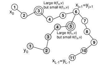
Figure 1: For every vertex $v$ such that $f_{X}\left(v\right)\neq f_{Y}\left(v\right)$, either when snake $X$ flicks its tail $v$ is not hit with high probability, or when snake $Y$ flicks its tail $v$ is not hit with high probability.

One difficulty is that not all snakes are good; at best, a large fraction of them are.  We could try deleting all inputs $f_{X}$ such that $X$ is not good, but that might ruin some remaining inputs, which would then have fewer neighbors.  So we would have to delete those inputs as well, and so on ad infinitum.  What we need is basically a way to replace “all inputs” by “most inputs” in Theorems 4.5 and 4.8.

Fortunately, a simple graph-theoretic lemma can accomplish this.  The lemma (see Diestel [12, p.6] for example) says that any graph with average degree at least $k$ contains an induced subgraph with minimum degree at least $k/2$.  Here we prove a weighted analogue of the lemma.

Lemma 5.12.

Let $p\left(1\right),\ldots,p\left(m\right)$ be positive reals summing to $1$.  Also let $w\left(i,j\right)$ for $i,j\in\left\{1,\ldots,m\right\}$ be nonnegative reals satisfying $w\left(i,j\right)=w\left(j,i\right)$ and $\allowbreak\sum_{i,j}w\left(i,j\right)\geq r$.  Then there exists a nonempty subset $U\subseteq\left\{1,\ldots,m\right\}$ such that for all $i\in U$, $\sum_{j\in U}w\left(i,j\right)\geq rp\left(i\right)/2.$

Proof 5.13.

If $r=0$ then the lemma trivially holds, so assume $r>0$.  We construct $U$ via an iterative procedure.  Let $U\left(0\right)=\left\{1,\ldots,m\right\}$.  Then for all $t$, if there exists an $i^{\ast}\in U\left(t\right)$ for which

$$\sum_{j\in U\left(t\right)}w\left(i^{\ast},j\right)<\frac{r}{2}p\left(i^{\ast}\right),$$

then set $U\left(t+1\right)=U\left(t\right)\setminus\left\{i^{\ast}\right\}$.  Otherwise halt and return $U=U\left(t\right)$.  To see that the $U$ so constructed is nonempty, observe that when we remove $i^{\ast}$, the sum $\sum_{i\in U\left(t\right)}p\left(i\right)$ decreases by $p\left(i^{\ast}\right)$, while $\sum_{i,j\in U\left(t\right)}w\left(i,j\right)$ decreases by at most

$$\sum_{j\in U\left(t\right)}w\left(i^{\ast},j\right)+\sum_{j\in U\left(t\right)}w\left(j,i^{\ast}\right)<rp\left(i^{\ast}\right).$$

So since $\sum_{i,j\in U\left(t\right)}w\left(i,j\right)$ was positive to begin with, it must still be positive at the end of the procedure; hence $U$ must be nonempty.

We can now prove the main result of the section.

Theorem 5.14.

Suppose a snake drawn from $\mathcal{D}_{h,L}$ is $\varepsilon$-good with probability at least $9/10$.  Then

$$\operatorname*{RLS}\left(G\right)=\Omega\left(1/\varepsilon\right),~{}~{}~{}~{}~{}~{}\operatorname*{QLS}\left(G\right)=\Omega\left(\sqrt{1/\varepsilon}\right).$$

Proof 5.15.

Given a snake $X\in D_{h,L}$, we construct an input function $f_{X}$ as follows.  For each $v\in X$, let $f_{X}\left(v\right)=\min\left\{t:x_{t}=v\right\}$; and for each $v\notin X$, let $f_{X}\left(v\right)=\Delta\left(v,h\right)+L$ where $\Delta\left(v,h\right)$ is the distance from $v$ to $h$ in $G$.  Clearly $f_{X}$ so defined has a unique local minimum at $x_{0}$.  To obtain a decision problem, we stipulate that querying $x_{0}$ reveals an answer bit ($0$ or $1$) in addition to $f_{X}\left(x_{1}\right)$; the algorithm’s goal is then to return the answer bit.  Obviously a lower bound for the decision problem implies a corresponding lower bound for the search problem. Let us first prove the theorem in the case that all snakes in $D_{h,L}$ are $\varepsilon$-good.  Let $p\left(X\right)$ be the probability of drawing snake $X$ from $\mathcal{D}_{h,L}$.  Also, given snakes $X,Y$ and $j\in\left\{0,\ldots,L-1\right\}$, let $q_{j}\left(X,Y\right)$ be the probability that $X^{\ast}=Y$, if $X^{\ast}$ is drawn from $\mathcal{D}_{h,L}$ conditioned on agreeing with $X$ on all steps later than $j$.  Then define

$$w\left(X,Y\right)=\frac{p\left(X\right)}{L}\sum_{j=0}^{L-1}q_{j}\left(X,Y\right).$$

Our first claim is that $w$ is symmetric; that is, $w\left(X,Y\right)=w\left(Y,X\right)$.  It suffices to show that

$$p\left(X\right)q_{j}\left(X,Y\right)=p\left(Y\right)q_{j}\left(Y,X\right)$$

for all $j$.  We can assume $X$ agrees with $Y$ on all steps later than $j$, since otherwise $q_{j}\left(X,Y\right)=q_{j}\left(Y,X\right)=0$.  Given an $X^{\ast}\in D_{h,L}$, let $A$ denote the event that $X^{\ast}$ agrees with $X$ (or equivalently $Y$) on all steps later than $j$, and let $B_{X}$ (resp. $B_{Y}$) denote the event that $X^{\ast}$ agrees with $X$ (resp. $Y$) on steps $1$ to $j$.  Then

$$p\left(X\right)q_{j}\left(X,Y\right) =\Pr\left[A\right]\Pr\left[B_{X}|A\right]\cdot\Pr\left[B_{Y}|A\right]$$

$$=p\left(Y\right)q_{j}\left(Y,X\right).$$

Now let $E\left(X,Y\right)$ denote the event that $X\cap Y=S_{X,Y}$, where $S_{X,Y}$ is as in Definition 5.11.  Also, let $f_{X}$ be the input obtained from $X$ that has answer bit $0$, and $g_{X}$ be the input that has answer bit $1$.  To apply Theorems 4.5 and 4.8, take $\mathcal{A}=\left\{f_{X}:X\in D_{h,L}\right\}$ and $\mathcal{B}=\left\{g_{X}:X\in D_{h,L}\right\}$.  Then take $R\left(f_{X},g_{Y}\right)=w\left(X,Y\right)$ if $E\left(X,Y\right)$ holds, and $R\left(f_{X},g_{Y}\right)=0$ otherwise.  Given $f_{X}\in\mathcal{A}$ and $g_{Y}\in\mathcal{B}$ with $R\left(f_{X},g_{Y}\right)>0$, and letting $v$ be a vertex such that $f_{X}\left(v\right)\neq g_{Y}\left(v\right)$, we must then have either $v\notin X$ or $v\notin Y$.  Suppose the former case; then

$$\sum_{f_{X^{\ast}}\in\mathcal{A}~{}:~{}f_{X^{\ast}}\left(v\right)\neq g_{Y}\left(v\right)}R\left(f_{X^{\ast}},g_{Y}\right)$$

$$\leq\sum_{f_{X^{\ast}}\in\mathcal{A}~{}:~{}f_{X^{\ast}}\left(v\right)\neq g_{Y}\left(v\right)}\frac{p\left(Y\right)}{L}\sum_{j=0}^{L-1}q_{j}\left(Y,X^{\ast}\right)\leq\varepsilon p\left(Y\right),$$

since $Y$ is $\varepsilon$-good.  Thus

$$\theta\left(g_{Y},v\right)=\frac{\sum_{f_{X^{\ast}}\in\mathcal{A}~{}:~{}f_{X^{\ast}}\left(v\right)\neq g_{Y}\left(v\right)}R\left(f_{X^{\ast}},g_{Y}\right)}{\sum_{f_{X^{\ast}}\in\mathcal{A}}R\left(f_{X^{\ast}},g_{Y}\right)}\leq\frac{\varepsilon p\left(Y\right)}{9p\left(Y\right)/10}.$$

Similarly, if $v\notin Y$ then $\theta\left(f_{X},v\right)\leq 10\varepsilon/9$ by symmetry.  Hence

$$\upsilon_{\min} =\max_{\begin{subarray}{c}f_{X}\in\mathcal{A},~{}g_{Y}\in\mathcal{B},~{}v:\\ R\left(f_{X},g_{Y}\right)>0,\\ f_{X}\left(v\right)\neq g_{Y}\left(v\right)\end{subarray}}\min\left\{\theta\left(f_{X},v\right),\theta\left(g_{Y},v\right)\right\}\leq\frac{\varepsilon}{9/10},$$

$$\upsilon_{\operatorname*{geom}} =\max_{\begin{subarray}{c}f_{X}\in\mathcal{A},~{}g_{Y}\in\mathcal{B},~{}v:\\ R\left(f_{X},g_{Y}\right)>0,\\ f_{X}\left(v\right)\neq g_{Y}\left(v\right)\end{subarray}}\sqrt{\theta\left(f_{X},v\right)\theta\left(g_{Y},v\right)}\leq\sqrt{\frac{\varepsilon}{9/10}},$$

the latter since $\theta\left(f_{X},v\right)\leq 1$ and $\theta\left(g_{Y},v\right)\leq 1$ for all $f_{X},g_{Y}$ and $v$. We now turn to the general case, in which a snake drawn from $\mathcal{D}_{h,L}$ is $\varepsilon$-good with probability at least $9/10$.  Let $G\left(X\right)$ denote the event that $X$ is $\varepsilon$-good.  Take $\mathcal{A}^{\ast}=\left\{f_{X}\in\mathcal{A}:G\left(X\right)\right\}$ and $\mathcal{B}^{\ast}=\left\{g_{Y}\in\mathcal{B}:G\left(Y\right)\right\}$, and take $\allowbreak R\left(f_{X},g_{Y}\right)$ as before.  Then since

$$\sum_{X,Y~{}:~{}E\left(X,Y\right)}w\left(X,Y\right)\geq\sum_{X}\frac{9}{10}p\left(X\right)\geq\frac{9}{10},$$

by the union bound we have

$$\sum_{f_{X}\in\mathcal{A}^{\ast},~{}g_{Y}\in\mathcal{B}^{\ast}}R\left(f_{X},g_{Y}\right)$$

$$\geq\sum_{X,Y~{}:~{}G\left(X\right)\wedge G\left(Y\right)\wedge E\left(X,Y\right)}w\left(X,Y\right)$$

$$\quad\quad\quad-\sum_{X~{}:~{}\urcorner G\left(X\right)}p\left(X\right)-\sum_{Y~{}:~{}\urcorner G\left(Y\right)}p\left(Y\right)$$

$$\geq\frac{9}{10}-\frac{1}{10}-\frac{1}{10}=\frac{7}{10}.$$

So by Lemma 5.12, there exist subsets $\widetilde{\mathcal{A}}\subseteq\mathcal{A}^{\ast}$ and $\widetilde{\mathcal{B}}\subseteq\mathcal{B}^{\ast}$ such that for all $f_{X}\in\widetilde{\mathcal{A}}$ and $g_{Y}\in\widetilde{\mathcal{B}}$,

$$\sum_{g_{Y^{\ast}}\in\widetilde{\mathcal{B}}}R\left(f_{X},g_{Y^{\ast}}\right) \geq\frac{7p\left(X\right)}{20},$$

$$\sum_{f_{X^{\ast}}\in\widetilde{\mathcal{A}}}R\left(f_{X^{\ast}},g_{Y}\right) \geq\frac{7p\left(Y\right)}{20}.$$

So for all $f_{X},g_{Y}$ with $R\left(f_{X},g_{Y}\right)>0$, and all $v$ such that $f_{X}\left(v\right)\neq g_{Y}\left(v\right)$, either $\theta\left(f_{X},v\right)\leq 20\varepsilon/7$ or $\theta\left(g_{Y},v\right)\leq 20\varepsilon/7$.  Hence $\upsilon_{\min}\leq 20\varepsilon/7$ and $\upsilon_{\operatorname*{geom}}\leq\sqrt{20\varepsilon/7}$.

6 Specific Graphs

In this section we apply the ‘snake method’ developed in Section 5 to specific examples of graphs: the Boolean hypercube in Section 6.1, and the $d$-dimensional cubic grid (for $d\geq 3$) in Section 6.2.

6.1 Boolean Hypercube

Abusing notation, we let $\left\{0,1\right\}^{n}$ denote the $n$-dimensional Boolean hypercube—that is, the graph whose vertices are $n$-bit strings, with two vertices adjacent if and only if they have Hamming distance $1$.  Given a vertex $v\in\left\{0,1\right\}^{n}$, we let $v\left[0\right],\ldots,v\left[n-1\right]$ denote the $n$ bits of $v$, and let $v^{\left(i\right)}$ denote the neighbor obtained by flipping bit $v\left[i\right]$.  In this section we lower-bound $\operatorname*{RLS}\left(\left\{0,1\right\}^{n}\right)$ and $\operatorname*{QLS}\left(\left\{0,1\right\}^{n}\right)$.

Fix a ‘snake head’ $h\in\left\{0,1\right\}^{n}$ and take $L=2^{n/2}/100$.  We define the snake distribution $\mathcal{D}_{h,L}$ via what we call a coordinate loop, as follows.  Starting from $x_{0}=h$, for each $t$ take $x_{t+1}=x_{t}$ with $1/2$ probability, and $x_{t+1}=x_{t}^{\left(t\operatorname{mod}n\right)}$ with $1/2$ probability.  The following is a basic fact about this distribution.

Proposition 6.16.

The coordinate loop mixes completely in $n$ steps, in the sense that if $t^{\ast}\geq t+n$, then $x_{t^{\ast}}$ is a uniform random vertex conditioned on $x_{t}$.

We could also use the random walk distribution, following Aldous [3].  However, not only is the coordinate loop distribution easier to work with (since it produces fewer self-intersections), it also yields a better lower bound (since it mixes completely in $n$ steps, as opposed to approximately in $n\log n$ steps).

We first upper-bound the probability, over $X$, $j$, and $Y\left[j\right]$, that $X\cap Y\neq S_{X,Y}$ (where $S_{X,Y}$ is as in Definition 5.11).

Lemma 6.17.

Suppose $X$ is drawn from $\mathcal{D}_{h,L}$, $j$ is drawn uniformly from $\left\{0,\ldots,L-1\right\}$, and $Y\left[j\right]$ is drawn from $\mathcal{D}_{x_{j},j}$.  Then $\Pr_{X,j,Y\left[j\right]}\left[X\cap Y=S_{X,Y}\right]\geq 0.9999$.

Proof 6.18.

Call a disagreement a vertex $v$ such that

$$\min\left\{t:x_{t}=v\right\}\neq\min\left\{t^{\ast}:y_{t^{\ast}}=v\right\}.$$

Clearly if there are no disagreements then $X\cap Y=S_{X,Y}$.  If $v$ is a disagreement, then by the definition of $\mathcal{D}_{h,L}$ we cannot have both $t>j-n$ and $t^{\ast}>j-n$.  So by Proposition 6.16, either $y_{t^{\ast}}$ is uniformly random conditioned on $X$, or $x_{t}$ is uniformly random conditioned on $Y\left[j\right]$.  Hence $\Pr_{X,j,Y\left[j\right]}\left[x_{t}=y_{t^{\ast}}\right]=1/2^{n}$.  So by the union bound,

$$\Pr_{X,j,Y\left[j\right]}\left[X\cap Y\neq S_{X,Y}\right]\leq\frac{L^{2}}{2^{n}}=0.0001.$$

We now argue that, unless $X$ spends a ‘pathological’ amount of time in one part of the hypercube, the probability of any vertex $v$ being hit when $X$ flicks its tail is small.  To prove this, we define a notion of sparseness, and then show that (1) almost all snakes drawn from $\mathcal{D}_{h,L}$ are sparse (Lemma 6.20), and (2) sparse snakes are unlikely to hit any given vertex $v$ (Lemma 6.22).

Definition 6.19.

Given vertices $v,w$ and $i\in\left\{0,\ldots,n-1\right\}$, let $\Delta\left(x,v,i\right)$ be the number of steps needed to reach $v$ from $x$ by first setting $x\left[i\right]:=v\left[i\right]$, then setting $x\left[i-1\right]:=v\left[i-1\right]$, and so on.  (After we set $x\left[0\right]$ we wrap around to $x\left[n-1\right]$.)  Then $X$ is sparse if there exists a constant $c$ such that for all $v\in\left\{0,1\right\}^{n}$ and all $k$,

$$\left|\left\{t:\Delta\left(x_{t},v,t\operatorname{mod}n\right)=k\right\}\right|\leq cn\left(n+\frac{L}{2^{n-k}}\right).$$

Lemma 6.20.

If $X$ is drawn from $\mathcal{D}_{h,L}$, then $X$ is sparse with probability $1-o\left(1\right)$.

Proof 6.21.

For each $i\in\left\{0,\ldots,n-1\right\}$, the number of $t\in\left\{0,\ldots,L-1\right\}$ such that $t\equiv i\left(\operatorname{mod}n\right)$ is at most $L/n$.  For such a $t$, let $E_{t}^{\left(v,i,k\right)}$ be the event that $\Delta\left(x_{t},v,i\right)\leq k$; then $E_{t}^{\left(v,i,k\right)}$ holds if and only if

$$x_{t}\left[i\right]=v\left[i\right],\ldots,x_{t}\left[i-k+1\right]=v\left[i-k+1\right]$$

(where we wrap around to $x_{t}\left[n-1\right]$ after reaching $x_{t}\left[0\right]$).  This occurs with probability $2^{k}/2^{n}$ over $X$.  Furthermore, by Proposition 6.16, the $E_{t}^{\left(v,i,k\right)}$ events for different $t$’s are independent.  So let

$$\mu_{k}=\frac{L}{n}\cdot\frac{2^{k}}{2^{n}};$$

then for fixed $v,i,k$, the expected number of $t$’s for which $E_{t}^{\left(v,i,k\right)}$ holds is at most $\mu_{k}$.  Thus by a Chernoff bound, if $\mu_{k}\geq 1$ then

$$\Pr_{X}\left[\left|\left\{t:E_{t}^{\left(v,i,k\right)}\right\}\right|>cn\cdot\mu_{k}\right]<\left(\frac{e^{cn-1}}{\left(cn\right)^{cn}}\right)^{\mu_{k}}<\frac{1}{2^{2n}}$$

for sufficiently large $c$.  Similarly, if $\mu_{k}<1$ then

$$\Pr_{X}\left[\left|\left\{t:E_{t}^{\left(v,i,k\right)}\right\}\right|>cn\right]<\left(\frac{e^{cn/\mu_{k}-1}}{\left(cn/\mu_{k}\right)^{cn/\mu_{k}}}\right)^{\mu_{k}}<\frac{1}{2^{2n}}$$

for sufficiently large $c$.  By the union bound, then,

$$\left|\left\{t:E_{t}^{\left(v,i,k\right)}\right\}\right|\leq cn\cdot\left(1+\mu_{k}\right)=c\left(n+\frac{L}{2^{n-k}}\right)$$

for every $v,i,k$ triple simultaneously with probability at least $1-n^{2}2^{n}/2^{2n}=1-o\left(1\right)$.  Summing over all $i$’s produces the additional factor of $n$.

Lemma 6.22.

If $X$ is sparse, then for every $v\in\left\{0,1\right\}^{n}$,

$$\Pr_{j,Y}\left[v\in Y\left[j\right]\right]=O\left(\frac{n^{2}}{L}\right).$$

Proof 6.23.

By assumption, for every $k\in\left\{0,\ldots,n\right\}$,

$$\Pr_{j}\left[\Delta\left(x_{j},v,j\operatorname{mod}n\right)=k\right] \leq\frac{\left|\left\{t:\Delta\left(x_{t},v,t\operatorname{mod}n\right)=k\right\}\right|}{L}$$

$$\leq\frac{cn}{L}\left(n+\frac{L}{2^{n-k}}\right).$$

Consider the probability that $v\in Y\left[j\right]$ in the event that $\Delta\left(x_{j},v,j\operatorname{mod}n\right)=k$.  Clearly

$$\Pr_{Y}\left[v\in\left\{y_{j-n+1},\ldots,y_{j}\right\}\right]=\frac{1}{2^{k}}.$$

Also, Proposition 6.16 implies that for every $t\leq j-n$, the probability that $y_{t}=v$ is $2^{-n}$.  So by the union bound,

$$\Pr_{Y}\left[v\in\left\{y_{0},\ldots,y_{j-n}\right\}\right]\leq\frac{L}{2^{n}}.$$

Then $\Pr_{j,Y}\left[v\in Y\left[j\right]\right]$ equals

$$\sum_{k=0}^{n}\left(\begin{array}[c]{c}\Pr_{j}\left[\Delta\left(x_{j},v,j\operatorname{mod}n\right)=k\right]\cdot\\ \Pr_{Y}\left[v\in Y\left[j\right]~{}|~{}\Delta\left(x_{j},v,j\operatorname{mod}n\right)=k\right]\end{array}\right)$$

$$\leq\sum_{k=0}^{n}\frac{cn}{L}\left(n+\frac{L}{2^{n-k}}\right)\left(\frac{1}{2^{k}}+\frac{L}{2^{n}}\right)=O\left(\frac{cn^{2}}{L}\right)$$

as can be verified by breaking the sum into cases and doing some manipulations.

The main result follows easily:

Theorem 6.24.

$$\operatorname*{RLS}\left(\left\{0,1\right\}^{n}\right)=\Omega\left(\frac{2^{n/2}}{n^{2}}\right),~{}~{}\operatorname*{QLS}\left(\left\{0,1\right\}^{n}\right)=\Omega\left(\frac{2^{n/4}}{n}\right).$$

Proof 6.25.

Take $\varepsilon=n^{2}/2^{n/2}$.  Then by Theorem 5.14, it suffices to show that a snake $X$ drawn from $\mathcal{D}_{h,L}$ is $O\left(\varepsilon\right)$-good with probability at least $9/10$.  First, since

$$\Pr_{X,j,Y\left[j\right]}\left[X\cap Y=S_{X,Y}\right]\geq 0.9999$$

by Lemma 6.17, Markov’s inequality shows that

$$\Pr_{X}\left[\Pr_{j,Y\left[j\right]}\left[X\cap Y=S_{X,Y}\right]\geq\frac{9}{10}\right]\geq\frac{19}{20}.$$

Second, by Lemma 6.20, $X$ is sparse with probability $1-o\left(1\right)$, and by Lemma 6.22, if $X$ is sparse then

$$\Pr_{j,Y}\left[v\in Y\left[j\right]\right]=O\left(\frac{n^{2}}{L}\right)=O\left(\varepsilon\right)$$

for every $v$.  So both requirements of Definition 5.11 hold simultaneously with probability at least $9/10$.

6.2 Constant-Dimensional Grid Graph

In the Boolean hypercube case, we defined $\mathcal{D}_{h,L}$ by a ‘coordinate loop’ instead of the usual random walk mainly for convenience.  When we move to the $d$-dimensional grid, though, the drawbacks of random walks become more serious: first, the mixing time is too long, and second, there are too many self-intersections, particularly if $d\leq 4$.  Our snake distribution will instead use straight lines of randomly chosen lengths attached at the endpoints, as in Figure 2.

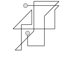
Figure 2: In $d=3$ dimensions, a snake drawn from $\mathcal{D}_{h,L}$ moves a random distance left or right, then a random distance up or down, then a random distance inward or outward, etc.

Let $G_{d,N}$ be a $d$-dimensional grid graph with $d\geq 3$.  That is, $G_{d,N}$ has $N$ vertices of the form $v=\left(v\left[0\right],\ldots,v\left[d-1\right]\right)$, where each $v\left[i\right]$ is in $\left\{1,\ldots,N^{1/d}\right\}$ (we assume for simplicity that $N$ is a $d^{th}$ power).  Vertices $v$ and $w$ are adjacent if and only if $\left|v\left[i\right]-w\left[i\right]\right|=1$ for some $i\in\left\{0,\ldots,d-1\right\}$, and $v\left[j\right]=w\left[j\right]$ for all $j\neq i$ (so $G_{d,N}$ does not wrap around at the boundaries).

We take $L=\sqrt{N}/100$, and define the snake distribution $\mathcal{D}_{h,L}$ as follows.  Starting from $x_{0}=h$, for each $T$ we take $x_{N^{1/d}\left(T+1\right)}$ identical to $x_{N^{1/d}T}$, but with the $\left(T\operatorname{mod}d\right)^{th}$ coordinate $x_{N^{1/d}\left(T+1\right)}\left[T\operatorname{mod}d\right]$ replaced by a uniform random value in $\left\{1,\ldots,N^{1/d}\right\}$.  We then take the vertices $x_{N^{1/d}T+1},\ldots,x_{N^{1/d}T+N^{1/d}-1}$ to lie along the shortest path from $x_{N^{1/d}T}$ to $x_{N^{1/d}\left(T+1\right)}$, ‘stalling’ at $x_{N^{1/d}\left(T+1\right)}$ once that vertex has been reached.  We call

$$\Phi_{T}=\left(x_{N^{1/d}T},\ldots,x_{N^{1/d}T+N^{1/d}-1}\right)$$

a line of vertices, whose direction is $T\operatorname{mod}d$.  As in the Boolean hypercube case, we have:

Proposition 6.26.

$\mathcal{D}_{h,L}$ mixes completely in $dN^{1/d}$ steps, in the sense that if $T^{\ast}\geq T+d$, then $x_{N^{1/d}T^{\ast}}$ is a uniform random vertex conditioned on $x_{N^{1/d}T}$.

Lemma 6.17 in Section 6.1 goes through essentially without change.

Definition 6.27.

Letting $\Delta\left(x,v,i\right)$ be as before, we say $X$ is sparse if there exists a constant $c$ (possibly dependent on $d$) such that for all vertices $v$ and all $k$,

$$\left|\left\{t:\Delta\left(x_{t},v,\left\lfloor t/N^{1/d}\right\rfloor\operatorname{mod}d\right)=k\right\}\right|$$

$$\leq\left(c\log N\right)\left(N^{1/d}+\frac{L}{N^{1-k/d}}\right).$$

Lemma 6.28.

If $X$ is drawn from $\mathcal{D}_{h,L}$, then $X$ is sparse with probability $1-o\left(1\right)$.

Lemma 6.29.

If $X$ is sparse, then for every $v\in G_{d,N}$,

$$\Pr_{j,Y}\left[v\in Y\left[j\right]\right]=O\left(\frac{N^{1/d}\log N}{L}\right),$$

where the big-$O$ hides a constant dependent on $d$.

The proofs of Lemmas 6.28 and 6.29 are omitted from this abstract, since they involve no new ideas beyond those of Lemmas 6.20 and 6.22.  Taking $\varepsilon=\left(\log N\right)/N^{1/2-1/d}$ we get, by the same proof as for Theorem 6.24:

Theorem 6.30.

Neglecting a constant dependent on $d$, for all $d\geq 3$

$$\operatorname*{RLS}\left(G_{d,N}\right) =\Omega\left(\frac{N^{1/2-1/d}}{\log N}\right),$$

$$\operatorname*{QLS}\left(G_{d,N}\right) =\Omega\left(\sqrt{\frac{N^{1/2-1/d}}{\log N}}\right).$$

7 Acknowledgments

I thank Andris Ambainis for suggesting an improvement to Proposition 3.3; David Aldous, Christos Papadimitriou, Yuval Peres, and Umesh Vazirani for discussions during the early stages of this work; and Ronald de Wolf and the anonymous reviewers for helpful comments.

References

• [1] S. Aaronson.  Quantum lower bound for the collision problem, Proc. ACM STOC, pp. 635–642, 2002.  quant-ph/0111102.
• [2] D. Aharonov and O. Regev.  Approximating the shortest and closest vector in a lattice to within $\sqrt{n}$ are in $\mathsf{NP}\cap\mathsf{coNP}$, unpublished.
• [3] D. Aldous.  Minimization algorithms and random walk on the d-cube, Annals of Probability 11(2):403–413, 1983.
• [4] A. Ambainis.  Polynomial degree vs. quantum query complexity, Proc. IEEE FOCS, pp. 230–239, 2003.  quant-ph/0305028.
• [5] A. Ambainis.  Quantum lower bounds by quantum arguments, J. Comput. Sys. Sci. 64:750–767, 2002.  Earlier version in STOC’2000.  quant-ph/0002066.
• [6] A. Ambainis.  Talk at the Banff Centre, Banff, Canada, June 18, 2003.
• [7] T. Baker, J. Gill, and R. Solovay.  Relativizations of the P=?NP question, SIAM J. Comput. 4:431–442, 1975.
• [8] R. Beals, H. Buhrman, R. Cleve, M. Mosca, and R. de Wolf.  Quantum lower bounds by polynomials, Proc. IEEE FOCS, pp. 352–361, 1998.  quant-ph/9802049.
• [9] C. Bennett, E. Bernstein, G. Brassard, and U. Vazirani. Strengths and weaknesses of quantum computing, SIAM J. Comput. 26(5):1510–1523, 1997.  quant-ph/9701001.
• [10] H. Buhrman, R. Cleve, R. de Wolf, and Ch. Zalka.  Bounds for small-error and zero-error quantum algorithms, Proc. IEEE FOCS, pp. 358–368, 1999.  cs.CC/9904019.
• [11] H. Buhrman and R. de Wolf.  Complexity measures and decision tree complexity: a survey, Theoretical Comput. Sci. 288:21–43, 2002.
• [12] R. Diestel.  Graph Theory (2nd edition), Springer-Verlag, 2000.
• [13] S. Droste, T. Jansen, and I. Wegener.  Upper and lower bounds for randomized search heuristics in black-box optimization, ECCC TR03-048, 2003.
• [14] C. Dürr and P. Høyer.  A quantum algorithm for finding the minimum, 1996.  quant-ph/9607014.
• [15] E. Farhi, J. Goldstone, S. Gutmann, J. Lapan, A. Lundgren, and D. Preda.  A quantum adiabatic evolution algorithm applied to random instances of an NP-complete problem, Science 292:472–476, 2001.  quant-ph/0104129.
• [16] D. S. Johnson, C. H. Papadimitriou, and M. Yannakakis.  How easy is local search?, J. Comput. Sys. Sci. 37:79–100, 1988.
• [17] I. Kerenidis and R. de Wolf.  Exponential lower bound for 2-query locally decodable codes via a quantum argument, Proc. ACM STOC, pp. 106–115, 2003.  quant-ph/0208062.
• [18] D. C. Llewellyn and C. Tovey.  Dividing and conquering the square, Discrete Appl. Math 43:131–153, 1993.
• [19] D. C. Llewellyn, C. Tovey, and M. Trick.  Local optimization on graphs, Discrete Appl. Math 23:157–178, 1989.  Erratum: 46:93–94, 1993.
• [20] N. Megiddo and C. H. Papadimitriou.  On total functions, existence theorems, and computational complexity, Theoret. Comp. Sci. 81:317–324, 1991.
• [21] C. H. Papadimitriou.  Talk at UC Berkeley, February 6, 2003.
• [22] M. Santha and M. Szegedy.  Quantum and classical query complexities of local search are polynomially related, this Proceedings, 2004.
• [23] Y. Shi.  Quantum lower bounds for the collision and the element distinctness problems, Proc. IEEE FOCS, pp. 513–519, 2002.  quant-ph/0112086.