Entanglement and quantum fluctuations

Abstract

We discuss maximum entangled states of quantum systems in terms of quantum fluctuations of all essential measurements responsible for manifestation of entanglement. Namely, we consider maximum entanglement as a property of states, for which quantum fluctuations come to their extreme.

In spite of a great progress in investigation and implementation of quantum entanglement, it still remains an enigmatic phenomenon, which is in need of accurate definition and disclosure of mathematical structure hidden behind it. The urgency of this is caused by the discovery of quantum cryptography 1 and quantum teleportation 2 that put entanglement at the very heart of quantum information processing and quantum computing (e.g., see Ref. 3 ).

As usually, the first thing to settle is to separate the essential from accidental. In the case of entanglement, this touches upon even the very definition, which still remains intuitive at great extent. In fact, the concept of entanglement was formed under strong influence of bipartite systems that have transparent mathematical structure provided by the Schmidt decomposition 4 .

Probably, the definition of entanglement that the most experts are agreeing with is as follows.

”Quantum entanglement is a subtle nonlocal correlation among the parts of a quantum system that has no classical analog. Thus, entanglement is best characterized and quantified as a feature of the system that cannot be created through local operations that act on the different parts separately, or by means of classical communication among the parts.” (See Ref. 5 ).

The assigning primary importance to the quantum correlations, having no classical analog, seems to be the most essential in the intuitive definitions of entanglement. In particular, just these correlations are responsible for information transmission in quantum channels 6 .

At the same time, the assumption of nonlocality, which is important for quantum communication processing, leads to a loss in generality. In particular, this requirement is meaningless in the case of entanglement in Bose-Einstein condensate because of the strong overlap of wave functions of individual atoms 7 . Besides that, it leaves aside the single-particle entanglement with respect to intrinsic degrees of freedom 8 ; 9 ; 10 .

The entanglement is also defined in terms of violation of classical realism described by the Bell-type inequalities 11 and Greenberger-Horne-Zeilinger (GHZ) conditions 12 . This means the violation of local classical constrains on the correlation of measurements performed on different parts of the system. In fact, violation of these constrains indicates the quantum nature of states and can be observed for unentangled states as well. An example is provided by coherent states 9 that represent an exact antithesis to entanglement.

In turn, the requirement of nonseparability of states that is often considered as a definition, in reality is not a sufficient condition of entanglement 13 . An example of nonseparable unentangled state is considered below.

An important property of entangled states is that one can change the amount of entanglement by a certain operations such as the Lorentz bust 14 and SLOCC (stochastic local operations assisted by classical communications) 15 ; 16 ; 17 . In particular, this means that all entangled states can be constructed from the maximum entangled (ME) states through the use of these operations 17 . Thus, if ME states are well defined, all other entangled states can be constructed.

The main aim of this note is to discuss a novel definition of ME states and its consequences.

From the intuitive definitions, it follows that the maximum entanglement should be considered as an extreme property of quantum states maximally remote from the ”classical reality” (classical bonds on correlation of measurements). Such a ”remoteness” can be naturally specified in terms of quantum fluctuations of observables.

As a matter of fact, the principle difference between the classical and quantum levels of description of physical systems consists just in the existence of quantum fluctuations (uncertainties) in the latter case, caused by the interpretation of observables in terms of Hermitian operators. The total uncertainty of all essential measurements performed over a physical system can be used as a measure of remoteness of a state of this system from the classical reality.

We choose to interpret ME state of a given system as that, providing the maximum remoteness from the classical reality.

To cast this definition into a rigorous form, consider a quantum system $S$ (not necessarily a nonlocal one) defined in the Hilbert space ${\mathbb{H}}(S)$. Let $\{M_{i}\}$ be a set of all essential measurements. The choice of the essential observables depends on the physical measurements we are going to perform over the system, or, what is the same, on the Hamiltonians, which are accessible for the manipulation with quantum states. Let $\psi\in{\mathbb{H}}(S)$ be a pure state. Then, the result of quantum measurement $M_{i}$ is specified by the expectation value

$$\langle M_{i}\rangle=\langle\psi|M_{i}|\psi\rangle$$ (1)

and variance (uncertainty)

$$V_{i}(\psi)\equiv\langle(\Delta M_{i})^{2}\rangle=\langle\psi|M_{i}^{2}|\psi\rangle-\langle\psi|M_{i}|\psi\rangle^{2},$$ (2)

describing quantum fluctuations. In the case of mixed state with the density matrix $\rho$, instead of (1) and (2) we get

$$\langle M_{i}\rangle=Tr(\rho M_{i}),\quad V_{i}(\rho)=Tr[\rho(\Delta M_{i})^{2}],$$ (3)

respectively.

We choose to specify the remoteness of quantum states from the classical reality by the total variance that has the form

$${\mathbb{V}}(\psi)=\sum_{i}V_{i}(\psi),$$ (4)

in the case of pure states, and

$${\mathbb{V}}(\rho)=\sum_{i}V_{i}(\rho),$$ (5)

in the case of mixed states.

In the spirit of our philosophy, we define ME of pure states in ${\mathbb{H}}(S)$ by the condition

$${\mathbb{V}}(\psi_{ME})=\max_{\psi\in{\mathbb{H}}(S)}{\mathbb{V}}(\psi).$$ (6)

In the case of mixed states, Eq. (6) is replaced by the following

$${\mathbb{V}}(\rho_{ME})=\max_{\rho}{\mathbb{V}}(\rho).$$ (7)

This definition means that ME states have the maximum scale of quantum fluctuations of all essential measurements. Eqs. (6) and (7) represent a variational principle for maximum entanglement similar in a sense to the maximum entropy principle in statistical mechanics. In particular, this principle permits us to understand how to prepare a persistent ME state, which is necessary for teleportation and other quantum information processes. First, we should exert influence upon the system to achieve the state with maximum scale of quantum fluctuations. Then, the energy of the system should be decreased up to a (local) minimum under the condition of retention of the fluctuation scale. The possible realization of the process in atom-photon system was discussed in Refs. 18 ; 19 .

In a special case of interest, when the enveloping algebra of the Lie algebra of all essential measurements ${\mathcal{L}}(M)$ contains a uniquely defined Casimir operator

$$\hat{\mathbf{C}}=\sum_{i}M^{2}_{i}={\mathbf{C}}\times\mathbb{I},$$ (8)

where $\mathbb{I}$ is the unit operator, the conditions (6) and (7) can be represented in a different form. Namely, it follows from Eqs. (2)-(5) and (8) that the maximum in (6) and (7) is achieved if

$$\forall i\quad\langle M_{i}\rangle=0.$$ (9)

Then, the maximum total variance takes the form

$${\mathbb{V}}_{max}={\mathbf{C}}.$$ (10)

It should be mentioned that it was observed in Ref. 20 that ME states obey the condition (9), which can be used as an operational definition of maximum entanglement.

To illustrate the definition of ME states (4) and condition (9), consider a system of $N$ qubits defined in the Hilbert space

$${\mathbb{H}}_{2,N}=({\mathbb{H}}_{2})^{N}.$$

A pure state $\psi\in{\mathbb{H}}_{2,N}$ has the form

$$|\psi\rangle=\sum\psi_{\ell_{1}\ell_{2}\cdots\ell_{N}}\mathbf{e}_{\ell_{1}}\otimes\mathbf{e}_{\ell_{2}}\otimes\cdots\otimes\mathbf{e}_{\ell_{N}},$$ (11)

where $\mathbf{e}_{\ell}=|\ell\rangle$, $\ell=0,1$, are the base vectors in ${\mathbb{H}}_{2}$. The dynamic symmetry group $G$ in the two-dimensional space ${\mathbb{H}}_{2}$ is $G=SU(2)$. At the same time, the local measurements are provided by the Pauli operators 21

$$\left\{\begin{array}[]{ll}\sigma_{1}=&|0\rangle\langle 1+|1\rangle\langle 0|\\ \sigma_{2}=&-i(|0\rangle\langle 1|-|1\rangle\langle 0|)\\ \sigma_{3}=&|0\rangle\langle 0|-|1\rangle\langle 1|\end{array}\right.$$ (15)

that form a representation of the infinitesimal generators of the $SL(2,{\mathbb{C}})$ algebra ${\mathcal{L}}^{c}$. The corresponding dynamic symmetry group $G^{c}=\exp({\mathcal{L}}^{c})$ is the $SL(2,{\mathbb{C}})$ group, which is known to be the complexification of $G=SU(2)$.

It should be stressed that the complexification of the dynamic group plays here very important role 8 . In particular, SLOCC in an $N$-partite system is identified with the complexification $G^{c}=\prod_{i}SL({\mathbb{H}}_{i})$ of the dynamic symmetry group $G=\prod_{i}SU({\mathbb{H}}_{i})$ 16 ; 17 . The complexification of the spin group $G=SU(2)$ also emerges as Lorentz group, locally isomorphic to $G^{c}=SL(2,{\mathbb{C}})$, in study of relativistic transformation of entanglement 14 .

The condition of maximum entanglement (9) imposes a certain restrictions on the multidimensional matrix 22 $[\psi]$ of coefficients in (11). Namely, the parallel slices of $[\psi]$ should be orthogonal and have the same norm. This result can also be considered as the necessary and sufficient condition of ME states 8 .

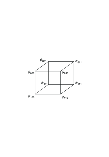
Figure 1: Structure of the three-dimensional matrix $[\psi]$ of three qubits. Vertices of the cube are associated with the coefficients $\psi_{ijk}$ in Eq. (11) at $N=3$.

Consider the three-qubit system ($N=3$). In this case, $[\psi]$ is a three-dimensional matrix (cube) shown in Fig. 1. The parallel slices are represented by the faces of the cube. Consider, for example, the parallel faces $(\psi_{000},\psi_{010},\psi_{100},\psi_{110})$ and $(\psi_{001},\psi_{011},\psi_{101},\psi_{111})$. The condition of orthogonality then gives the equations

$$Re(\psi_{000}\psi_{001}^{*}+\psi_{010}\psi_{011}^{*}+\psi_{110}\psi_{111}^{*}+\psi_{100}\psi_{101}^{*}) =0,$$

$$Im(\psi_{000}\psi_{001}^{*}+\psi_{010}\psi_{001}^{*}+\psi_{110}\psi_{111}^{*}+\psi_{100}\psi_{101}^{*}) =0,$$

that coincide with the conditions $\langle\sigma_{1}^{(3)}\rangle=0$ and $\langle\sigma_{2}^{(3)}\rangle=0$, where the superscript indicates the measuring party. In turn, the equation

$$|\psi_{000}|^{2}+|\psi_{010}|^{2}+|\psi_{110}|^{2}+|\psi_{100}|^{2}$$

$$=|\psi_{001}|^{2}+|\psi_{011}|^{2}+|\psi_{111}|^{2}+|\psi_{101}|^{2},$$

specifying the equality of the corresponding norms, comes from the condition $\langle\sigma_{3}^{(3)}\rangle=0$. All other conditions in (9) can be considered in the same way.

It is seen that the conditions (9) in the case of $N$-qubit system give $3\times N$ equations. One more equation comes from the normalization of (11). At the same time, the number of complex elements in $[\psi]$ is equal to $\dim{\mathbb{H}}_{2,N}=2^{N}$, which corresponds to $2\times 2^{N}$ real parameters. Since $2^{N+1}>3\times N+1$ at $N\geq 2$, any bipartite and multipartite system of two qubits has infinitely many ME states. Among them, the ME states forming a basis in ${\mathbb{H}}_{2,N}$ are important. Such a basis can be constructed in the following way. Consider first the generic ME state of $N$ qubits

$$\frac{1}{\sqrt{2}}(|00\cdots 0\rangle\pm|11\cdots 1\rangle)=\frac{1}{\sqrt{2}}\sum_{\ell=0}^{1}\bigotimes_{j=1}^{N}|\ell\rangle_{j}.$$ (16)

It is easily seen that the two states (13) obey the condition (9). The examples at $N=2$ and $N=3$ are provided by the Bell and GHZ states, respectively. The basis of ME states in ${\mathbb{H}}_{2,N}$ can be generated by the action of the local cyclic permutation operator

$${\mathcal{C}}_{2}=|0\rangle\langle 1|+|1\rangle\langle 0|$$ (17)

on the generic states (13) $(2^{N-1}-1)$ times (also see Ref. 2 ). Here the operator (14) formally coincides with $\sigma_{1}$ in (12). In the case of qudits ($d$ degrees of freedom per party), this operator takes the form

$${\mathcal{C}}_{d}=|0\rangle\langle 1|+\cdots+|d-1\rangle\langle 0|$$

so that ${\mathcal{C}}^{d}={\mathbb{I}}$.

Consider now a few important corollaries of the above definition of ME states.
$\bullet$ Corollary 1. The classification of quantum states according to the scale of quantum fluctuations is known since the discussion of coherent states (e.g., see 23 ; 24 ). The coherent states have the minimum scale of quantum fluctuations and therefore they are considered as almost classical states. Thus, by definition, ME states represent an exact antithesis to coherent states.
$\bullet$ Corollary 2. The definition of ME states (6) or (7) is independent on whether the system is nonlocal or not. For example, it can be used to specify ME states of a particle with respect to internal degrees of freedom. An example is provided by $\pi$-mesons that are built from the up $u$ and down $d$ quarks as follows 25

$$\pi^{+}\rightarrow u\bar{d},\quad\pi^{-}\rightarrow\bar{u}d,\quad\pi_{0}\rightarrow\frac{u\bar{u}-d\bar{d}}{\sqrt{2}}.$$

The first two particles $\pi^{\pm}$ correspond to the coherent states of internal (quark) degrees of freedom, while $\pi^{0}$ is specified by ME state with respect to quarks. Since these two states have quite different levels of quantum fluctuations, $\pi^{0}$ meson should be less stable than $\pi^{\pm}$. In fact, the ratio of lifetimes is $\tau_{0}/\tau_{\pm}\sim 3\times 10^{-9}$. The single-particle entangled states are possible if the number of internal degrees of freedom exceeds two (single qutrit etc.).
$\bullet$ Corollary 3. The definition of ME states (6) can also be applied to the photon field, when the dynamic symmetry is specified by the Weyl-Heisenberg group. Choosing the measurements as the field quadratures

$$q=\frac{1}{2}(a+a^{+}),\quad p=\frac{-i}{2}(a-a^{+}),\quad[a,a^{+}]=1$$

and employing condition (9), it is easily seen that the Fock number state $|n\rangle$ and squeezed vacuum state give $\langle q\rangle=\langle p\rangle=0$ and provide the total variances

$${\mathbb{V}}_{Fock}=(2n+1)/2,\quad{\mathbb{V}}_{squeez}=(2\cosh r-1)/2,$$

respectively. Here $r$ is the squeezing parameter. A certain difference between the variances is caused by the fact that the Weyl-Heisenberg algebra has no uniquely defined Casimir operator. The number and squeezed vacuum state represents a kind of parametric ME states because the scale of quantum fluctuations is specified by the parameters $n$ and $r$, respectively. The real ME states are achieved in the limit $n,r\rightarrow\infty$.

Of course, some other entangled states of light, specified by the measurements belonging to the $SU(N)$ subalgebras in the Weyl-Heisenberg algebra and corresponding to the polarization and angular moment of photons, can also be considered in terms of definition (6) and (7).
$\bullet$ Corollary 4. The total variance (4) cannot be used as a measure of entanglement. The unentangled states may manifest even more quantum fluctuations than entangled states but not ME states. For example, the three-qubit $W$ state 16 has ${\mathbb{V}}_{W}=8+2/3$. The maximum entangled GHZ state has ${\mathbb{V}}_{GHZ}=9$, so that the level of quantum fluctuations in $W$ state is quite close to maximum. At the same time, $W$ state is not entangled because the 3-tangle 26 , which is similar to Cayley’s hyperdeterminant 27 and is an entangled monotone in the case of three qubits, is equal to zero. Thus, nonseparable $W$ state is not entangled. In turn, the state

$$|\psi_{x}\rangle=x(|000\rangle+|111\rangle)+y(|001\rangle+|110\rangle),$$ (18)

where $x^{2}+y^{2}=1/2$, is entangled but not maximum entangled at $x\neq 1/2,1/\sqrt{2}$. In the intervals $0.122<x<0.5$ and $0.5<x<0.696$, we get ${\mathbb{V}}_{x}<{\mathbb{V}}_{W}$.
$\bullet$ Corollary 5. The definition (6) and possibility to construct the entangled states from ME states by means of SLOCC put the notion of entanglement within the framework of geometric invariant theory 8 (concerning geometric invariant theory, see Ref. 28 ). This permits us to introduce a new universal measure of entanglement which is the length of minimal vector in complex orbit 8

$$\mu(\psi)=\min_{g\in G^{c}}|g\psi|^{2}.$$ (19)

Here $\psi\in{\mathbb{H}}(S)$ is a state of quantum system $S$ and $G^{c}$ is the complexified dynamic symmetry group in ${\mathbb{H}}(S)$. This measure represents an entangled monotone, which is equal to zero for unentangled states and achieves maximum for ME states. The measure (16) coincides with the concurrence (determinant of $[\psi]$ in (11) at $N=2$) in the case of two qubits and with the square root of 3-tangle for three qubits. It can also be calculated in the case of four qubits (all geometric invariants in four-qubit system were calculated in Ref. 29 ). The description of entanglement and its proper measure (not necessarily of maximum entanglement) within the framework of geometric invariant theory deserves a special, more detailed discussion.

Summarizing, we should stress that the definition of ME states in terms of extreme quantum fluctuations agrees with that based on the consideration of quantum correlations, whose maximum in many cases can be expressed in terms of condition (9) as well. At the same time, definition in terms of the variational principle (6) or (7) is more general and has an evident heuristic advantage. It lays bare the physical essence of the phenomenon as the manifestation of quantum fluctuations at their extreme and reveals the mathematical structure hidden behind the entanglement.

The most of examples in this note were referred to pure states. They can be easily generalized on the case of mixed states because the latter can be treated as a pure state of a certain doublet, consisting of the system $S$ and its ”mirror image” 30 .

References

- (1) C.H. Bennett and G. Brassard, in Proc. IEEE Int. Conf. Computers, Systems and Signal Processing (1984).
- (2) C.H. Bennett, G. Brassard, C. Crepeau, R. Josa, A. Peres, and W.K. Wooters, Phys. Rev. Lett. 70, 1895 (1993).
- (3) C.H. Bennett and P.W. Shor, IEEE Trans. Inform. Theory 44, 2724 (1998).
- (4) A. Ekert and P.L. Knight, Am. J. Phys. 63, 415 (1995).
- (5) Quantum Information Science. NSF Workshop, October 28-29, 1999, Arlington, Virginia; www.nsf.gov/pubs/2000/nsf00101/nsf00101.htm.
- (6) A. Zeilinger, Phil. Trns. Roy. Soc. London 1733, 2401 (1997); Found. Phys. 29, 631 (1999).
- (7) A.J. Leggett, Rev. Mod. Phys. 73, 307 (2001).
- (8) A.A. Klyachko, E-print quant-ph/0206012.
- (9) A.A. Klyachko and A.S. Shumovsky, J. Opt. B 5, S322 (2003).
- (10) Y.-H. Kim, E-print quant-ph/0303125.
- (11) J.S. Bell, Physics 1, 195 (1964); J. Clauser, M. Horne, A. Shimony, and R. Holt, Phys. Rev. Lett. 23, 880 (1969); D.N. Mermin, Am. J. Phys. 66, 753; M. Ardehali, Phys. Rev. A 46, 5375; A.V. Belinskii and D.N. Klyshko, Phys. Uspehi 36, 653 (1993).
- (12) D.M. Greenberger, M. Horne, and A. Zeilinger, in Bell’s Theorem, Quantum Theory, and Concepts of Universe, edited by M. Kafatos (Kluwer Academic, Dordreht, 1989); D.M. Greenberger, M. Horne, A. Shimony and A. Zeilinger, Am. J. Phys. 58, 1131 (1990).
- (13) M. Horodecki, P. Horodecki, and R. Horodecki, Phys. Rev. Lett. 80, 5239 (1998).
- (14) A. Peres, P.F. Scudo, and D.R. Terno, Phys. Rev. Lett. 88, 230402 (2002); A. Peres and D.R. Terno, E-print quant-ph/0208128; A.J. Bergou, R.M. Gingrich, and C. Adami, E-print quant-ph/0302095.
- (15) C.H. Bennett, H.J. Bernstein, S. Popescu, and B. Schumacher, E-print quant-ph/9511030; C.H. Bennett, S. Popescu, D. Rohrlich, J.A. Smolin, and A.V. Thapaliya, Phys. Rev. A 63, 012307 (2001).
- (16) W. Dür, G. Vidal, and J.I. Cirac, Phys. Rev. A 62, 062314 (2000).
- (17) F. Verstraete, J. Dehaene, B. De Moor, and H. Verschelde, Phys. Rev. A 65, 052112 (2002).
- (18) M.A. Can, A.A. Klyachko, and A.S. Shumovsky, Appl. Phys. Lett. 81, 5072 (2002).
- (19) Ö. Çakır, M.A. Can, A.A. Klyachko, and A.S. Shumovsky, Phys. Rev. A (in press); E-print quant-ph/0211157.
- (20) M.A. Can, A.A. Klyachko, and A.S. Shumovsky, Phys. Rev. A 66, 022111 (2002).
- (21) M.A. Nielsen and I.L. Chuang, Quantum Computation and Quantum Information (Cambridge University Press, Cambridge, 2000).
- (22) Concerning the multidimensional matrices, see: I.M. Gelfand, M.M. Kapranov, and A.V. Zelevinsky, Determinants, Resultants, and Multidimensional Determinants (Birkhauser, Boston MA, 1994).
- (23) L. Delbargo and J.R. Fox, J. Phys. A 10, 1233 (1970).
- (24) A. Perelomov, Generalized Coherent States and Their Applications (Springer, Berlin, 1986).
- (25) K. Huang, Quarks, Leptons and Gauge Fields (World Scientific, Singapore, 1982).
- (26) V. Coffman, J. Kundu, and W.K. Wooters, Phys. Rev. A 61, 052306 (2000).
- (27) A. Miyake, E-print quant-ph/0206111.
- (28) E. Vinberg and V. Popov, Invariant Theory (Springer, Berlin, 1992).
- (29) J.-G. Luque and J.-Y. Thibon, Phys. Rev. A 67, 042303 (2003).
- (30) Y. Takahashi and H. Umezawa, Int. J. Mod. Phys. B 10, 1755 (1996).