Distillation of continuous-variable entanglement with optical means

Abstract

We present an event-ready procedure that is capable of distilling Gaussian two-mode entangled states from a supply of weakly entangled states that have become mixed in a decoherence process. This procedure relies on passive optical elements and photon detectors distinguishing the presence and the absence of photons, but does not make use of photon counters. We identify fixed points of the iteration map, and discuss in detail its convergence properties. Necessary and sufficient criteria for the convergence to two-mode Gaussian states are presented. On the basis of various examples we discuss the performance of the procedure as far as the increase of the degree of entanglement and two-mode squeezing is concerned. Finally, we consider imperfect operations and outline the robustness of the scheme under non-unit detection efficiencies of the detectors. This analysis implies that the proposed protocol can be implemented with currently available technology and detector efficiencies.

I Introduction

The key requirement in essentially all practical applications of quantum information science is to protect the coherence of quantum states against decoherence induced by the uncontrolled influences of an environment. Entangled states of composite quantum systems, in particular, deteriorate typically into mixed quantum states with mere classical correlations. Decoherence accompanies to some extent any attempt to distribute entangled states that have been prepared using some local interaction. The first obvious strategy to minimize this effect is to try to reduce the interaction with the environment, e.g., by using glass fibers with a long characteristic absorption length when distributing photonic entanglement.

This strategy is, however, not enough in many cases. If one intends to share entanglement over arbitrary distances, entanglement must in some way be extracted out of the only weakly entangled quantum systems. Under the key word entanglement distillation such strategies have been developed Bennett , most notably the iterative distillation schemes that work for spin-$1/2$ or qubit systems. In such schemes, entanglement is distilled out of a supply of weakly entangled pairs of quantum systems by means of local operations and classical communication. Such protocols have been proposed as theoretical concepts Bennett , and discussed under the assumption of imperfect devices HansHans . They form the basis of the theoretical concept of the distillable entanglement Rains , which clarifies the notion of entanglement as a resource. All the proposed protocols share nevertheless one property: they are experimentally very difficult to implement. First steps towards the full experimental realization of a distillation scheme very recently been taken Exp , based on earlier theoretical work on optical distillation protocols in the finite-dimensional setting Fin . However, it seems fair to say that the practical realization of full-scale entanglement distillation remains one of the key challenges of the field.

In this paper we present a feasible alternative to entanglement distillation in the finite-dimensional setting. We present a procedure that is capable of entanglement distillation and purification employing systems with canonical coordinates, or so-called continuous-variable systems such as light modes or harmonic oscillator systems. The scheme that we present is as such an extension of the Gaussification scheme of Ref. Gaussify . In this paper, we investigate the power of this procedure to distill states that have become mixed as a result of a decoherence process Scheel . More specifically, we investigate whether Gaussian states that originate for example from two-mode squeezed states TMSSTheory ; TMSSTheory2 ; tmss ; GExp that underwent a decoherence process can be transformed back into highly entangled Gaussians using feasible local operations and classical communication only.

The result that, highly entangled and often even pure Gaussian states can be extracted from a supply of weakly entangled mixed states, appears to be in strong contrast to the no-go-theorems concerning the distillation of Gaussian states with Gaussian operations NoGo ; NoGo2 ; NoGo3 . However, the central idea is to leave the Gaussian setting in a first preparation step, and only in the course of the iteration the resulting states converge towards a final Gaussian state. In this sense one can sneak through a loophole left open by the statements demonstrating the impossibility of entanglement distillation when staying entirely within the Gaussian setting. It has been shown that the general use of non-Gaussian operations allow for entanglement purification gaussdistillability . However, it should be noted that the scheme presented here endeavors to employ non-Gaussian operations in a minimal way, namely only in the first step. Also, merely detectors are required that distinguish the presence and absence of photons. The resulting procedure yields finally the desired output: the states are approximately (i) pure, (ii) Gaussian, and (iii) highly entangled. As such, this protocol could serve as a quantum privacy amplification protocol in continuous-variable PreskillCrypto ; cryptography entanglement-based quantum key distribution. Needless to say, privacy amplification to pure states is only possible in case of an error-free implementation of the required steps. In any practical realization, this is of course not possible. One of the crucial numbers specifying to what extent the procedure can achieve pure final states is the detection efficiency of the used photon detectors. Yet, the purity of the final states is no necessary requirement for quantum privacy amplification to function.

It should be noted that this procedure may well have significant advantages compared to schemes in the finite-dimensional setting, even when one is indifferent to whether the resulting states are entangled in polarization or continuous degrees of freedom, and is only interested in some form of highly entangled states of light. The procedure is event-ready, in the sense that one has a classical signal at hand indicating success, and in principle, one can use the resulting states on the basis of this measurement. Photon counters, or set-ups where the photon number can be inferred in retrospect from the outcomes of measurements on all modes including the output modes, as well as controlled-not operations are not required. Also, no post-processing is necessary dependent on the measurement outcomes, which constitutes an advantage in iterative protocols where the output of one step is the input of the next step. But in turn, the final state that one obtains can obviously not be the same maximally entangled state for all inputs, as for finite-dimensional procedures this is often the case, one reason being that the maximally entangled state does not even exist in state space. There is no measure of the quality of the output available as the fidelity with respect to a maximally entangled state.

We have decided to split our analysis into several parts, in a hierarchy of abstraction versus practicability: Following the introduction of the procedure in Section II, we will investigate the power of the procedure in abstract terms. Section III will be dedicated to this analysis, where we will assume the applied quantum operations to be error-free. The procedure can be conceived as the continuous-variable analogue of the finite-dimensional quantum privacy amplification procedure Bennett . We will present statements identifying the fixed points of the iteration map: we will find that exactly the Gaussians centred in phase space form the set of fixed points. We will investigate convergence properties, and in particular present necessary and sufficient criteria for convergence to a pure entangled Gaussian state. The proofs – some of them are technically involved – will be presented in a self-contained section in the Appendix. The degree of entanglement and two-mode squeezing properties of the output will be investigated in great detail, and several examples will be discussed.

Section IV is concerned with the non-Gaussian preparatory step in the absence and presence of decoherence. This step also relies only on photon detectors and passive linear optics. In Section V we will then discuss the situation when the performed operations are not noiseless. The most relevant parameter here is the detection efficiency of the photon detectors. We will present the iteration map, and will investigate by numerical means what output states should be expected asymptotically after many iteration steps. In an experiment that realizes, say, a single step of the distillation procedure, further sources of imperfection play a role. This is the third part of the analysis. These additional imperfections, including dark counts of the detectors and mode matching issues will be sketched at the end of Section V and will be discussed in great detail in a forthcoming publication. Also, the quantum privacy amplification capabilities in the presence of noisy apparata will be discussed elsewhere. The present paper concentrates to a large extent to flesh out what can be achieved in an asymptotic setting, or in a protocol where many steps can be implemented: as such it shows that continuous variable entanglement can be distilled, even when resorting to the most feasible class of operations. For imperfect detectors, yet, it is shown that even after a small number of steps and for fairly low detection efficiencies, the degree of entanglement can be significantly increased. Finally, in Section VI we summarise what we have achieved, and sketch what further steps could be taken towards the implementation of continuous-variable distillation schemes with continuous variables.

II The procedure

The procedure makes use of only beam splitters and photon detectors distinguishing the presence and absence of photons. The iteration amounts to a very elementary operation, and it will only turn out to be technical to characterize its properties concerning convergence. From a supply of two-mode squeezed states, one prepares two-mode states $\rho$ in a first step. The state $\rho$ is assumed to be non-Gaussian in the sense that its associated characteristic function or Wigner function is not a Gaussian in phase space. This step can be conceived as the preparatory part, this preparation will be discussed in more detail in Section V. Pairs $\rho\otimes\rho$ of such non-Gaussian states $\rho$ are then mixed at a $50:50$ beam splitter, yielding a state

$$(U\otimes U)(\rho\otimes\rho)(U\otimes U)^{\dagger},$$ (1)

where the beam splitters are reflected by unitaries vogelwelsch

$$U=T^{a_{1}^{\dagger}a_{1}}e^{-R^{\ast}a_{2}^{\dagger}a_{1}}e^{Ra_{2}a_{1}^{\dagger}}T^{-a_{2}^{\dagger}a_{2}},$$ (2)

where we set $T=R=1/\sqrt{2}$. Two of the output modes are then directed into a photon detector, whose action is each associated with Kraus operators

$$E_{1}=|0\rangle\langle 0|,\,\,E_{2}={\mathbbm{1}}-|0\rangle\langle 0|,$$ (3)

where $|0\rangle$ denotes the state vector associated with the vacuum state. Note that the first operator is a Gaussian projector and the second merely the difference of two Gaussian operators, which is a very simple non-Gaussian operation indeed.

The state is kept in case of the vacuum outcome of both local detectors. The procedure is the Gaussification procedure of Ref. Gaussify , but now the input states are not necessarily pure states. The unnormalized final state after one step is given by

$$\langle 0,0|(U\otimes U)(\rho\otimes\rho)(U\otimes U)^{\dagger}|0,0\rangle.$$ (4)

The resulting two-mode states then form the basis of the next step. It is an iterative protocol, and it is event-ready, in the sense that one has a classical signal at hand which indicates whether the procedure was successful or not. No further post-processing has to be performed. The Gaussification procedure is depicted in Fig. 1.

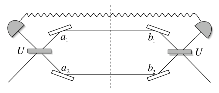
Figure 1: A single step of the protocol: two non-Gaussian states are mixed at a $50:50$ beam splitter. Two of the output modes are fed into photon detectors, the remaining two modes are kept in further steps, given a vacuum outcome in the detectors.

III Perfect devices

In this section we investigate the ideal situation where all operations can be implemented to perfect accuracy. In particular, perfect detection efficiencies are assumed, but later, this assumption will be relaxed. We first discuss the recurrence relation of the states, and then identify all fixed points of the map. We then investigate convergence, and give a necessary and sufficient criterion for convergence to a pure Gaussian two-mode state. Note that the general situation that we encounter here is different from the finite-dimensional setting. In the latter case, the fidelity with respect to a maximally entangled state is a meaningful measure of the quality of the output, for example the fidelity with respect to the singlet state of two qubits. Here, no such maximally entangled state exists, and consequently, the degree of squeezing, of entanglement, and the von-Neumann entropy characterizing purity are unbounded. Hence, a more complicated interplay should be expected. We state the quality of the output in terms of the degree of entanglement and squeezing of the output.

III.1 The iteration map

The iteration map takes as input a four-mode state, and has a two-mode state as output, which corresponds to the resulting state after the measurement, given that both measurement outcomes were appropriate. Let $\omega$ be a four-mode state; the iteration map ${\cal E}$ is then defined as

$${\cal E}(\omega)=\langle 0,0|(U\otimes U)\omega(U\otimes U)^{\dagger}|0,0\rangle.$$ (5)

The output of one step is the input of the next step, which gives rise to a sequence of states representing the output after a number of steps. The map that links one state with the subsequent one – given a positive outcome of the measurements – will be referred to as recursion relation.

The recursion relation can be stated in a transparent way as follows. The two-mode state $\rho$ can be represented in the number basis $\{|n\rangle:n\in{\mathbbm{N}}\}$ as

$$\rho=\sum_{s,t,n,m=0}^{\infty}\rho_{s,t;n,m}|s,t\rangle\langle n,m|.$$ (6)

The output $\rho^{\prime}={\cal E}(\rho\otimes\rho)$ can then be written as

$$\rho^{\prime}=\sum_{s,t,n,m=0}^{\infty}\rho^{\prime}_{s,t;n,m}|s,t\rangle\langle n,m|,$$ (7)

where

$$\rho^{\prime}_{a,b;c,d} = \sum_{s=0}^{a}\sum_{t=0}^{b}\sum_{n=0}^{c}\sum_{m=0}^{d}M_{a,b;c,d}^{s,t;n,m}$$ (8)

$$\times \rho_{s,t;n,m}\rho_{a-s,b-t;c-n,d-m}.$$

The coefficients $M_{a,b;c,d}^{s,t;n,m}$ are given by

$$M_{a,b;c,d}^{s,t;n,m} = 2^{-(a+b+c+d)/2}(-1)^{(a+b+c+d)-(s+t+n+m)}$$ (9)

$$\times \left[\binom{a}{s}\binom{b}{t}\binom{c}{n}\binom{d}{m}\right]^{1/2}.$$

Note that each number $\rho^{\prime}_{a,b;c,d}$ for some $a,b,c,d\in{\mathbbm{N}}$ is a polynomial in $\rho_{s,t;n,m}$ for $s\leq a$, $t\leq b$, $n\leq c$, and $m\leq d$ only. This is a quite helpful property as it implies that changes of coefficients associated with certain Fock numbers depend only on coefficients associated with smaller Fock numbers. This property will prove to be crucial in the formal proofs of convergence that are presented later on in this paper.

III.2 Fixed points of the map

The first task is to identify the fixed points of the iteration map: these are the states that are left unchanged under the operation. With fixed point we mean two-mode states $\rho$ for which there exists a $c\in(0,1]$ such that

$$\rho=c\;{\cal E}(\rho\otimes\rho).$$ (10)

The number $c$ reflects the fact that we do not require the output to be the appropriate one with unit probability. Some fixed points can easily be found. These are all two-mode Gaussian states with vanishing first moments. That this set of Gaussian states qualifies as being a set of fixed points becomes obvious in terms of the covariance matrices.

This can be formulated as follows. For a general $n$-mode system, let $R=(X_{1},P_{1},\ldots,X_{n},P_{n})$ be the vector consisting of the canonical coordinates of an $n$-mode system (only two and four-mode systems will be relevant). The canonical commutation relations (CCR) $[R_{j},R_{k}]=i\Sigma_{j,k}$ for $j,k=1,\ldots,2n$ give rise to the symplectic matrix

$$\Sigma=\bigoplus_{j=1}^{n}\left(\begin{array}[]{cc}0&1\\ -1&0\\ \end{array}\right).$$ (11)

If the second moments exist, then the covariance matrix $\gamma$ st , a real symmetric $2n\times 2n$-matrix, is defined as

$$\gamma_{j,k}=2\text{Re}\left(\text{Tr}[(R_{j}-\text{Tr}[R_{j}\rho])(R_{k}-\text{Tr}[R_{k}\rho])\rho]\right).$$ (12)

Every covariance matrix satisfies the Heisenberg uncertainty principle $\gamma+i\Sigma\geq 0$.

Symplectic transformations st such as the one corresponding to the application of the above beam splitters are reflected by transformations of the form

$$\gamma\longmapsto S\gamma S^{T}$$ (13)

with $S\in Sp(2n,{\mathbbm{R}})$, i.e., $S\Sigma S^{T}=\Sigma$ st . If the first moments vanish, the characteristic function $\chi:{\mathbbm{R}}^{2n}\longrightarrow{\mathbbm{C}}$ defined as $\chi(\xi)=\text{tr}[W_{\xi}\rho]$ of a Gaussian state $\rho$ can be written as

$$\chi(\xi)=e^{-(\xi^{T}\Sigma^{T}\gamma\Sigma\xi)/4},$$ (14)

where the Weyl displacement operator is given by

$$W_{\xi}=\exp(i\xi^{T}\Sigma R).$$ (15)

$\gamma$ is just the above covariance matrix. With this notation, the fact that Gaussians in the centre of phase space form fixed points becomes straightforward.

Proposition 1 (Gaussian states are fixed points)

Let $\rho$ be a Gaussian two-mode state with vanishing first moments. Then ${\cal E}(\rho\otimes\rho)=\rho$.

In fact, this set of fixed points is already exhaustive: there are no other fixed points that do not have the property of Proposition 1. This is quite a surprise, but a pleasant one, as it makes the characterisation of the fixed points very easy: the fixed points are exactly the Gaussian states with vanishing first moments, and there are no other states that are left unaffected by the iteration. The proof of this assertion can be found in Appendix A.

Proposition 2 (All fixed points are Gaussian)

Let $\rho$ be a two-mode state satisfying $c\;{\cal E}(\rho\otimes\rho)=\rho$ for some $c>0$. Then $\rho$ is a Gaussian state with vanishing first moments.

The proof of this statement – while being of central interest for the purposes of this paper – is quite technical and will for the sake of readability of the main text be presented in Appendix B. The property stated in Proposition 2 is an interesting feature of the iteration map: it is a Gaussian map and hence maps by definition all Gaussian states onto Gaussian states. But even when applied to general two-mode quantum states, the only fixed points of the map happen to be Gaussian states as well. No other state is left unchanged under the mixing at the beam splitters followed by the measurement.

III.3 Convergence

Once the fixed points have been specified, the next step is to see whether the procedure in fact converges to such a Gaussian state with vanishing first moments. So the question is under what constraints the procedure converges to a state at all – which is then one of the fixed points. We will also characterize fully those initial states, pure or mixed, for which convergence can be shown to an exactly pure Gaussian state.

The above protocol is probabilistic, and in the following convergence proofs it is assumed that it is successful in each step. This is to demonstrate that as a matter of principle, this procedure has the power of distilling entangled Gaussian states from a supply of non-Gaussian initial states. The closer the state approaches the fixed point, the smaller the improvement in quality in a step of our procedure. As every step of the procedure loses at least half of the partially entangled pairs that enter the iteration step one has to make a meaningful choice concerning the accuracy to which the envisioned entangled state can be achieved on the one hand and the rate with which this is possible on average on the other hand.

For a $\rho\in{\cal S}$, where ${\cal S}$ denotes the state space on ${\cal H}\otimes{\cal H}$, let ${\cal E}^{(1)}(\rho)$ be defined as

$${\cal E}^{(1)}(\rho)={\cal E}(\rho\otimes\rho),$$ (16)

and

$${\cal E}^{(i+1)}(\rho)={\cal E}({\cal E}^{(i)}(\rho)\otimes{\cal E}^{(i)}(\rho))$$ (17)

for $i\in{\mathbbm{N}}$. So ${\cal E}^{(i+1)}(\rho)$ is nothing than the unnormalized outcome of the procedure after $i+1$ steps of the iteration. The actual states are then

$$\rho^{(i)}=\frac{{\cal E}^{(i)}}{\text{tr}[{\cal E}^{(i)}]}.$$ (18)

The next result states when convergence to one of the fixed points can be expected.

To express the result in a concise manner, introduce a useful map, $B:{\cal S}\longrightarrow M_{4\times 4}$, which for any state $\rho$ allows one to construct a real symmetric $4\times 4$ matrix $B(\rho)$, with which we will characterize the convergence properties of the protocol. The map $B$ can be defined in terms of the matrix elements of $B(\rho)$ as follows:

$$B(\rho)_{1,1} = \frac{1}{2}\left(-(\sigma_{1,0,1,0}-1)+\sqrt{2}{\text{Re}}(\sigma_{2,0,0,0})\right)$$

$$B(\rho)_{2,2} = \frac{1}{2}\left(-(\sigma_{1,0,1,0}-1)-\sqrt{2}{\text{Re}}(\sigma_{2,0,0,0})\right)$$

$$B(\rho)_{3,3} = \frac{1}{2}\left(-(\sigma_{0,1,0,1}-1)+\sqrt{2}{\text{Re}}(\sigma_{0,2,0,0})\right)$$

$$B(\rho)_{4,4} = \frac{1}{2}\left(-(\sigma_{0,1,0,1}-1)-\sqrt{2}{\text{Re}}(\sigma_{0,2,0,0})\right)$$

$$B(\rho)_{1,2} = \frac{1}{\sqrt{2}}{\text{Im}}(\sigma_{2,0,0,0})$$

$$B(\rho)_{3,4} = \frac{1}{\sqrt{2}}{\text{Im}}(\sigma_{0,2,0,0})$$

$$B(\rho)_{1,3} = \frac{1}{2}\left(-{\text{Re}}(\sigma_{1,0,0,1})+{\text{Re}}(\sigma_{1,1,0,0})\right)$$

$$B(\rho)_{1,4} = \frac{1}{2}\left({\text{Im}}(\sigma_{1,0,0,1})+{\text{Im}}(\sigma_{1,1,0,0})\right)$$

$$B(\rho)_{2,3} = \frac{1}{2}\left(-{\text{Im}}(\sigma_{1,0,0,1})+{\text{Im}}(\sigma_{1,1,0,0})\right)$$

$$B(\rho)_{2,4} = \frac{1}{2}\left(-{\text{Re}}(\sigma_{1,0,0,1})-{\text{Re}}(\sigma_{1,1,0,0})\right)$$ (19)

where we define $\sigma=\rho/\rho_{0,0,0,0}$, which is the state $\rho$ normalized such that element $\sigma_{0,0,0,0}=1$ for states $\rho\in{\cal S}$ with $\rho_{0,0,0,0}=\langle 0,0|\rho|0,0\rangle>0$. The map is not defined for states with $\rho_{0,0,0,0}=0$, but that has no consequences for this discussion.

For a Gaussian two-mode state $\rho$, the $4\times 4$-matrix $B(\rho)$ is always invertible, and its covariance matrix is simply

$$\gamma=\Sigma^{T}B(\rho)^{-1}\Sigma+{\mathbbm{1}}_{4}.$$ (20)

Proposition 3 (Convergence to Gaussian states)

Let $\rho\in{\cal S}$. Then there exists a Gaussian two-mode state with vanishing first moments $\omega$ satisfying

$$\lim_{i\rightarrow\infty}\langle a,b|\left(\rho^{(i)}-\omega\right)|c,d\rangle=0$$ (21)

for all $a,b,c,d\in{\mathbbm{N}}_{0}$ if and only if both (i) $\langle 0,0|{\cal E}(\rho\otimes\rho)|0,0\rangle>0$, and (ii) $B(\rho^{(1)})$ is invertible.

The matrix

$$\Sigma^{T}B(\rho^{(1)})^{-1}\Sigma+{\mathbbm{1}}_{4}$$ (22)

with $\rho^{(1)}={\cal E}(\rho\otimes\rho)/\text{tr}[{\cal E}(\rho\otimes\rho)]$ is then the covariance matrix of the resulting Gaussian state to which the procedure converges (weakly). In other words, the procedure always converges to Gaussian two-mode states, whenever there is a non-vanishing success probability. The proof of this statement will be presented in Appendix C. The most interesting case is the situation where one can prove convergence to an exactly pure Gaussian state. This is the case when $\Sigma^{T}B(\rho^{(1)})^{-1}\Sigma+{\mathbbm{1}}_{4}$ is the covariance matrix of a pure Gaussian state. In this case, however, the necessary and sufficient criteria can be formulated in a more transparent manner. For imperfect detectors one will not achieve this goal exactly. From the perspective of the basic understanding of the procedure, however, necessary and sufficient conditions for convergence are instructive.

Proposition 4

(Necessary and sufficient conditions for convergence to pure Gaussians) Let $\rho\in{\cal S}$. Then there exists a pure two-mode Gaussian state $|\psi\rangle\langle\psi|$ centred in phase space satisfying

$$\lim_{i\rightarrow\infty}\langle a,b|\left(\rho^{(i)}-|\psi\rangle\langle\psi|\right)|c,d\rangle=0$$ (23)

for all $a,b,c,d\in{\mathbbm{N}}_{0}$ if and only if (i) $\rho_{0,0,0,0}>0$, (ii)

$$\rho_{1,0,1,0} = |\rho_{1,0,0,0}|^{2}/\rho_{0,0,0,0},$$ (24)

$$\rho_{0,1,0,1} = |\rho_{0,1,0,0}|^{2}/\rho_{0,0,0,0},$$ (25)

$$\rho_{1,0,0,1} = |\rho_{1,0,0,0}|^{2}/\rho_{0,0,0,0},$$ (26)

and (iii)

$$\left\|\begin{array}[]{cc}\sqrt{2}\frac{\rho_{2,0,0,0}}{\rho_{0,0,0,0}}-\frac{\rho_{1,0,0,0}^{2}}{\rho_{0,0,0,0}^{2}}&\frac{\rho_{1,1,0,0}}{\rho_{0,0,0,0}}-\frac{\rho_{1,0,0,0}\rho_{0,1,0,0}}{\rho_{0,0,0,0}}\\ \frac{\rho_{1,1,0,0}}{\rho_{0,0,0,0}}-\frac{\rho_{1,0,0,0}\rho_{0,1,0,0}}{\rho_{0,0,0,0}}&\sqrt{2}\frac{\rho_{0,2,0,0}}{\rho_{0,0,0,0}}-\frac{\rho_{1,0,0,0}^{2}}{\rho_{0,0,0,0}^{2}}\end{array}\right\|_{\infty}<1,$$ (29)

where $\|.\|_{\infty}$ denotes the spectral norm.

The proof of Proposition 4 can be found in Appendix D. In this sense the protocol can also work as a purification protocol. Not only the degree of entanglement and squeezing are increased, but also the von-Neumann entropy decreased. Note, however, that the conditions to convergence to exactly pure Gaussian states are fairly restrictive, and one will often encounter the situation that the states are almost pure. It can also happen that the degree of entanglement is significantly increased in the course of the procedure, but the von-Neumann entropy also increases.

Such a procedure would – if implemented with perfect physical devices – clearly lead to a perfect distillation procedure, and moreover, to the possibility of quantum privacy amplification for unconditionally secure quantum key distribution: if the state is a pure state, it cannot be entangled to any system of a third party, and the resulting states could be used to simply transmit a quantum state encoding the key. Needless to say, one would still have to apply classical methods to extract a secure key from the measurement outcomes, as the states exhibit only a finite squeezing, and hence, measurements of canonical coordinates by means of homodyne detection do not yield a deterministic outcome. This is, however, then entirely due to the Gaussian character of the quantum state and not due to an eavesdropper.

Note that the second moments of the states do not remain constant during this procedure, as they are modified in the steps involving measurements. For example, the only states with the second moments of a Gaussian pure state is a Gaussian state itself. Hence, the ‘Gaussification’ of the states is not merely a mixing to a Gaussian state, by virtue of the law of large numbers.

III.4 Examples

We will now turn to discussing a number of examples to visualize the procedure. For a number of initial states we will discuss the degree of entanglement after a single step and compare it with the degree of entanglement of the Gaussian state the sequence of states converges to. We start by giving an example for pure states, and then turn to mixed initial states.

Example 1: Let $\rho\in{\cal S}$ be the (pure) state with

$$\rho_{0,0,0,0} = 1/(1+\varepsilon^{2}),$$ (31)

$$\rho_{1,1,0,0} = \rho_{0,0,1,1}=\varepsilon/(1+\varepsilon^{2}),$$

$$\rho_{1,1,1,1} = \varepsilon^{2}/(1+\varepsilon^{2}),$$

with $\varepsilon\in[0,1)$, and $\rho_{a,b,c,d}=0$ with $a,b,c,d\in{\mathbbm{N}}_{0}$ otherwise. The sequence of outputs converges to a Gaussian pure state, the covariance matrix of which can be evaluated according to Proposition 3. Depending on the value of $\varepsilon$, the degree of entanglement that can be achieved will be different. This degree of entanglement will now and in the following be quantified in terms of the logarithmic negativity logneg , which is for a state $\rho$ of a bi-partite system defined as

$$E_{N}(\rho)=\log_{2}\|\rho^{\Gamma}\|_{1},$$ (32)

where $\|.\|_{1}$ denotes the trace-norm, and $\rho^{\Gamma}$ is the partial transpose of $\rho$ QuantNote . The negativity has been shown to be monotone under local operations with classical communication lognegmon ; lognegmon2 . The logarithmic negativity is an upper bound for the distillable entanglement, grasping the resource character of entanglement. For Gaussian states, as we encounter here, the logarithmic negativity has moreover a clearcut physical interpretation in terms of an asymptotic cost function PPT . For the specific initial state as in Eq. (31), Fig. 2 displays the behavior the logarithmic negativity of the initial state $\rho$, and of the Gaussian state the sequence of states converges to as a function of $\varepsilon\in[0,1)$. Note that the corresponding expressions can be evaluated analytically, by virtue of Proposition 3.

For $\varepsilon\rightarrow 1$ the logarithmic negativity of the resulting Gaussian state diverges, which reflects the fact that with unit detection efficiencies, one could in principle prepare arbitrarily entangled and squeezed states in this manner. This holds, as should be noted, also in the single-mode case, and one may prepare states with an arbitrary degree of single-mode squeezing. Technical limitations, however, will limit the degree of squeezing that is actually attainable, as will be discussed later.

Figure 2: The logarithmic negativity of the resulting states for an initial state $\rho$ as specified in Eq. (31). Depicted is the logarithmic negativity of the Gaussian state the sequence converges to (straight line), i.e., the degree of entanglement after ’infinitely many steps’, (ii) of the output state after a single iteration of the protocol (dashed line), and (iii) of the initial state $\rho$ itself (dotted line). Note that the increase of entanglement is already significant in a single step of the procedure. For infinitely many iterations and $\varepsilon\rightarrow 1$ the degree of entanglement diverges.

Example 2: As another example, let us consider the state $\rho\in{\cal S}$ with

$$\rho_{0,0,0,0} = \rho_{1,1,0,0}=\rho_{0,0,1,1}=\rho_{1,1,1,1}$$ (33)

$$= 1/(2+\varepsilon),$$

$$\rho_{0,1,0,1} = \varepsilon/(2+\epsilon)$$

with $\varepsilon\in[0,\infty)$, and $\rho_{a,b,c,d}=0$ otherwise. This state is mixed for all values $\varepsilon\in(0,\infty)$. Fig. 3 depicts again the value of the logarithmic negativity of the initial state, after a single iteration step and after ’infinitely many’ iterations.

Figure 3: The logarithmic negativity of the resulting states for initial states $\rho$ as in Eq. (33). Again, the straight line shows the negativity of the Gaussian state the sequence converges to, with diverging logarithmic negativity as $\varepsilon$ approaches zero. The dashed line represents the logarithmic negativity after a single step, whereas the dotted line is the logarithmic negativity of the original state.

Figure 4: As Fig. 3 for the initial state as in Eq. (34).

Example 3: The third example is $\rho\in{\cal S}$ with

$$\rho_{0,0,0,0} = 1/(1+\varepsilon^{2}),\,\,\rho_{1,1,0,0}=\rho_{0,0,1,1}=\varepsilon/(2+2\varepsilon^{2})$$

$$\rho_{1,1,1,1} = \varepsilon^{2}/(1+\varepsilon^{2})$$ (34)

with $\varepsilon\in[0,1)$, and $\rho_{a,b,c,d}=0$ otherwise. Again, we depict the degree of entanglement in Fig. 4. This is a set of initial states for which exact convergence to a pure Gaussian state is guaranteed by Proposition 4 for all values of $\varepsilon$. In Fig. 5, the von-Neumann entropy $S(\omega)=-\text{tr}[\omega\log_{2}\omega]$ for states $\omega$ is displayed, again as a function of $\varepsilon$, characterizing the purity of the resulting states. Note that the state does not only become more entangled, but also less mixed in the course of the protocol.

Figure 5: This figure depicts the von-Neumann entropy of the output as a function of $\varepsilon\in[0,1)$, for the initial state as in Eq. (34). The dotted line corresponds to the initial state itself, and the dashed lines show the von-Neumann entropy after one (dashed), two (dashed with longer dashing), and four steps (solid line). The limiting von-Neumann entropy vanishes exactly, as the conditions for Proposition 4 are met. Note that for very mixed initial states the von-Neumann entropy can first increase, to then decrease again in further steps.

Example 4: As a mere graphical illustration of the procedure we represent the states that are encountered in the procedure in phase space. More specifically, for the initial state $\rho$ as in Example 1 with $\varepsilon=0.6$ we investigate the Wigner function of the single-mode states of the reduced state of one mode alone for the initial state, and the state after one and two steps. The Wigner function $W:{\mathbbm{R}}^{2}\longrightarrow{\mathbbm{R}}$ is the Fourier transform of the characteristic function,

$$W(\xi)=\frac{1}{(2\pi)^{2}}\int e^{i\xi^{T}\Sigma\eta}\chi(\eta)d^{2}\eta.$$ (35)

Fig. 6 shows the Wigner function of $\text{tr}_{B}[\rho]$, $\text{tr}_{B}[\rho^{(1)}]$, and $\text{tr}_{B}[\rho^{(2)}]$. While initially, the Wigner function is far from being a Gaussian in phase space, its non-Gaussian features disappear quickly.

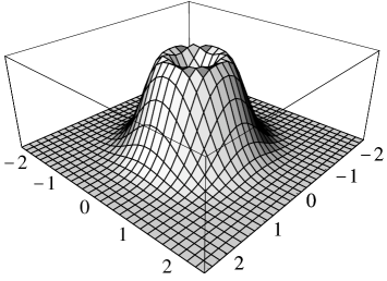
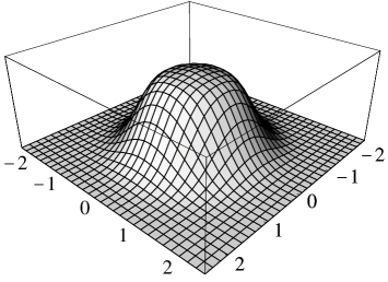
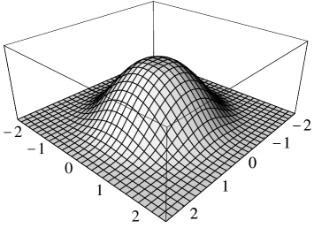
Figure 6: The Wigner function of the reduced state of one system initially and after one and two steps for the initial state as in Eq. (31).

III.5 Achievable squeezing

Another relevant figure is the degree of two-mode squeezing that one can achieve. For a Gaussian state $\rho$ with covariance matrix $\gamma$, one of the standard definitions for the degree of squeezing translates into the language of covariance matrices to

$$E_{S}(\rho)=\max\left\{-\log\lambda_{\text{min}}(\gamma),0\right\}$$ (36)

where $\lambda_{\text{min}}$ denotes the smallest eigenvalue. Roughly speaking, one compares the variance with respect to some canonical coordinate of this state with the one of the vacuum. For example, for the two-mode squeezed state $\rho$ with a covariance matrix of the form (41) with

$$\xi=\cosh(2r),\,\,\zeta=\sinh(2r),$$ (37)

$r\in[0,\infty)$ being the ordinary two-mode squeezing parameter, we arrive at $E_{S}(\rho)=r$. In terms of dB, the degree of squeezing is related to $E_{S}(\rho)$ according to $2E_{S}(\rho)/\log(10)$. For a two-mode state, this gives the total degree of squeezing. To distinguish genuine two-mode squeezing from locally available single-mode squeezing, one may consider for a two-mode state with $4\times 4$ covariance matrix of the block form

$$\gamma=\left(\begin{array}[]{cc}\gamma_{A}&\gamma_{C}\\ \gamma_{C}^{T}&\gamma_{B}\end{array}\right)$$ (38)

the quantity

$$E_{TS}(\rho)=\max\left\{-\log\lambda_{\text{min}}((S_{A}\oplus S_{B})\gamma(S_{A}\oplus S_{B})^{T}),0\right\},$$

where $S_{A},S_{B}\in Sp(2,{\mathbbm{R}})$ are chosen in such a way such that

$$S_{A}\gamma_{A}S_{A}^{T}=\alpha{\mathbbm{1}}_{2},\,\,\,S_{B}\gamma_{B}S_{B}^{T}=\beta{\mathbbm{1}}_{2}$$ (40)

with $\alpha,\beta\geq 1$, and $S_{A}\gamma_{C}S_{B}^{T}$ is diagonal. This is the degree of squeezing after the state has been locally brought to a form corresponding to a Gibbs state with appropriate local symplectic transformations (that can in particular include also single-mode squeezing).

IV Preparatory step

The above procedure takes non-Gaussian states as input. If one starts off with a Gaussian state, a preparatory step is clearly necessary. Such a step has been described in Ref. Gaussify . In principle, any other protocol preparing the states that are suitable in the above procedure would be appropriate as well. The one presented here has the advantage that it does not leave the scope of the paper, in that only the possibility of preparing Gaussian states is assumed, and the use of dichotomic photon detectors with high efficiency, which do not resolve the photon number.

IV.1 The preparation procedure

Let us assume that one has two-mode squeezed states at hand, which are Gaussian states the covariance matrix of which is of the form

$$\gamma=\left(\begin{array}[]{cccc}\xi&0&\zeta&0\\ 0&\xi&0&-\zeta\\ \zeta&0&\xi&0\\ 0&-\zeta&0&\xi\end{array}\right),$$ (41)

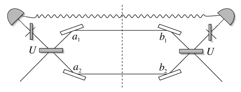
Figure 10: A single step of the protocol for detection efficiencies smaller than one. The detection efficiency less than unity is incorporated by placing perfect detectors behind a beam splitter.

where $\zeta^{2}=\xi^{2}-1$, $\xi\in(0,\infty]$. The numbers $\xi,\zeta$ characterize the degree of two-mode squeezing, as in Eq. (37). It has been shown in Ref. Gaussify that with the procedure as in Fig. 10, with the appropriate choice for $\xi$ and for the transmittivity $T$ and reflectivity $R$ of the beam splitter $V$, the resulting mixed two-mode state can be made arbitrarily close in trace-norm to a maximally entangled state in the subspace isomorphic to ${\mathbbm{C}}^{2}\otimes{\mathbbm{C}}^{2}$ with state vector $|0,0\rangle+\lambda|1,1\rangle/(1+\lambda^{2})^{1/2}$ for any value of $\lambda\in[0,1)$. This state can be used as input of the procedure. Taking this as input of the procedure of Section II, the sequence of states will converge to a pure state with an arbitrarily large degree of entanglement, as well as an arbitrary degree of two-mode squeezing.

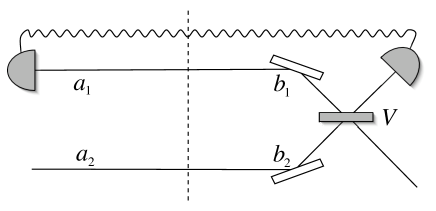
Figure 7: The preparatory step which resembles very much the step of an iteration in the Gaussification scheme. Given two specimens of two-mode squeezed states, measurements are performed on two of the four modes. However, now the outcome is accepted in case that both detectors click, corresponding to the Kraus operators $E_{2}={\mathbbm{1}}-|0\rangle\langle 0|$. The beam splitter $V$ is not a $50:50$ beam splitter, but one that has an appropriately tuned reflectivity and transmittivity.

IV.2 The full protocol under decoherence

Yet, such states are not available in the presence of a decoherence process. Once locally prepared, two-mode squeezed states or other entangled Gaussian states will deteriorate into weakly entangled mixed states. The decoherence dynamics we are interested in, i.e., transmission through an absorbing fiber, does not alter the Gaussian character of the state scheelwelsch , and it acts in effect as a Gaussian channel Channel . We assume that both modes are affected in the same manner.

Starting from the two-mode state with covariance matrix $\gamma$ as in Eq. (41), the state after the decoherence process is a Gaussian state with a covariance matrix of the same simple form, but with the roles of $\xi$ and $\zeta$ being replaced by

$$\xi\longmapsto 1+\theta^{2}(\xi-1),\,\,\,\,\zeta\longmapsto\theta^{2}\zeta,$$ (42)

$\theta\in[0,1]$ specifying the strength of the decoherence process. The value $\theta=1$ corresponds to no losses at all. It is a tedious but straightforward calculation to show (compare, e.g., Ref. Nonlin ) that for each value of $\theta$, one can find a choice for $\xi$ and the transmittivity $T$ and reflectivity $R$ such that the resulting state becomes arbitrarily close in trace-norm to $\rho\in{\cal S}$ with

$$\rho_{0,0,0,0} = 1/(1+\lambda^{2}\varepsilon+\lambda^{2}),$$ (43)

$$\rho_{1,1,0,0} = \rho_{0,0,1,1}=\lambda\rho_{0,0,0,0},$$ (44)

$$\rho_{1,1,1,1} = \lambda^{2}\rho_{0,0,0,0},$$ (45)

$$\rho_{0,1,0,1} = \varepsilon\lambda^{2}\rho_{0,0,0,0},$$ (46)

with

$$\varepsilon=(1-\theta^{2})/\theta^{2},$$ (47)

and $\rho_{a,b,c,d}=0$ otherwise. Any value for the number $\lambda\in[0,1]$ can be achieved. For $\lambda=1$ this is nothing but the state of Example 2 given in Eq. (33). The negativity after a number of steps of the Gaussification protocol for this initial state has already been depicted in Fig. 3. If one implements the full procedure, including the preparatory step and one or several instances of the whole procedure, it is certainly the relevant figure to compare the resulting degree of entanglement with the one before even the preparatory step has been taken. However, the initial two-mode squeezed states that have to be transmitted before the preparatory step has a negligible degree of entanglement: in order to better and better approximate the state of the form as in Eq. (33), less and less entanglement is needed, at the expense that the achievable rate decreases. Therefore, in principle, with perfect detection efficiencies as considered in this section, one can encounter an arbitrarily large entanglement gain. Also, note that the largest increase in entanglement per step occurs already in the preparatory step – this is specific for this case of perfect detectors. Figs. 8 and 9 show the degree of squeezing and entanglement that can be asymptotically achieved as a function of $\lambda$ for several values of $\theta\in[0,1]$.

Figure 8: The degree of two-mode squeezing for the Gaussian to which convergence is encountered, as a function of $\lambda\in[0,1)$, for $\theta=1$ (solid line), $\theta=0.9$ (dashed line), and $\theta=0.8$ (dotted line).

Figure 9: As Fig. 8, but for the degree of entanglement in terms of the achievable logarithmic negativity.

V Imperfect devices

Until now, it was assumed that the devices that are being used are noiseless and error free. We have seen that with such devices, distillation to highly entangled Gaussian states is indeed possible. This is the continuous-variable analogue to quantum privacy amplification in the finite-dimensional case. In any practical realization of such a scheme, however – just as in the case of finite systems such as qubits – the performance of the scheme depends very much on to what accuracy the operations can be performed. The most important number here is the detector efficiency of the photon detectors.

Needless to say, there are other potential sources of error: there is no intrinsic need for storing light in fiber loops, but nevertheless, losses even in short fibers cannot be avoided. If the scheme is not implemented entirely within fibers, losses are due to the coupling into the fiber. Then, in the entire paper we have discussed single modes only, and not broadband squeezed states TMSSTheory . In a practical realization, mode-matching problems will occur. Finally, dark counts of the photon detectors must be included in the treatment: here, however, it turns out that dark counts are much less problematic as one is tempted to think on intuitive grounds. Firstly, in the Gaussification step the only effect of dark counts is that one accidently does not accept the resulting state. This merely leads to a reduced rate of production of entangled states, but does not result in an increase of noise in the outputs. As the whole protocol is assumed to be implemented with a high repetition rate, this reduction of rate is acceptable. In the preparatory step dark counts do play a role. But even here, as the preparation requires a coincidence of several or many detectors in a very short time window (four in the simplest case), the dark count rate can in principle be made arbitrarily small. These further sources of errors will be discussed in a forthcoming paper. As has been pointed out in the introduction, in this paper, we concentrate on the most crucial source of error, the non-unit detection efficiency.

V.1 The iteration map

The case of imperfect detectors is modeled as follows, the usual projection operator onto the number state $|n\rangle\langle n|$ is replaced by

$$|n\rangle\langle n|\longmapsto\sum_{k=n}^{\infty}{k\choose n}\eta^{n}(1-\eta)^{k-n}|k\rangle\langle k|,$$ (48)

with $\eta\in[0,1]$. This formula has a representation in terms of a beam-splitter of transmittivity $T=\sqrt{\eta}$ placed in front of a detector with unit efficiency (see, e.g., Ref. K ). As before, let $\rho$ be some trace-class two-mode positive operator, i.e., a not necessarily normalized two-mode state. In the Fock basis, it can be represented as in Eq. (6). The resulting $\rho^{\prime}$ after one step of the procedure,

$$\rho^{\prime}={\cal E}_{T}(\rho\otimes\rho),$$ (49)

where ${\cal E}$ is replaced by the map ${\cal E}_{T}$ reflecting non-unit efficiency, can then be written as

$$\rho^{\prime}=\sum_{s,t,n,m=0}^{\infty}\rho^{\prime}_{s,t;n,m}|s,t\rangle\langle n,m|.$$ (50)

The new coefficients can be evaluated to be given by

$$\rho^{\prime}_{A,B;C,D}=\sum_{k,l=0}^{\infty}\sum_{a=0}^{A+k}\sum_{b=0}^{B+l}\sum_{c=0}^{C+k}\sum_{d=0}^{D+l}$$

$$\times \sum_{s=0}^{\min\{a,k\}}\sum_{u=0}^{\min\{b,l\}}\sum_{s^{\prime}=0}^{\min\{c,k\}}\sum_{u^{\prime}=0}^{\min\{d,l\}}$$

$$\times N_{A,B,C,D}^{a,b,c,d,s,u,s^{\prime},u^{\prime}}\rho_{a,b;c,d}\,\,\rho_{A+k-a,B+l-b,C+k-c,D+l-d},$$

where

$$N_{A,B,C,D}^{a,b,c,d,s,u,s^{\prime},u^{\prime}}=2^{-(A+B+C+D+2k+2l)/2}$$

$$\times (-1)^{A-a+B-b+C-c+D-d+s+u+s^{\prime}+u^{\prime}}(1-\eta)^{k+l}$$

$$\times \left[\binom{a}{s}\binom{k}{s}\binom{A+k-a}{k-s}\binom{A}{a-s}\right]^{1/2}$$

$$\times \left[\binom{b}{u}\binom{l}{u}\binom{B+l-b}{l-u}\binom{B}{b-u}\right]^{1/2}$$

$$\times \left[\binom{c}{s^{\prime}}\binom{k}{s^{\prime}}\binom{C+k-c}{k-s^{\prime}}\binom{C}{c-s^{\prime}}\right]^{1/2}$$

$$\times \left[\binom{d}{u^{\prime}}\binom{l}{u^{\prime}}\binom{D+l-d}{l-u^{\prime}}\binom{D}{d-u^{\prime}}\right]^{1/2}.$$

The case $\eta=1$ describes a detector with unit efficiency, and this expression reduces to the one described above.

V.2 Examples

The issue here is to what extent the noise introduced by imperfect photon detectors is harmful to the functioning of the protocol. Very low detection efficiencies obviously render the protocol less effective. Then, in each step of the iteration more entanglement is lost than concentrated. In turns out, however, that it is not necessary to have detectors with efficiencies very close to unity. Instead, with efficiencies that are achievable with present avalanche photodiodes, the degree of entanglement can in fact be increased in the actual Gaussification step. Astonishingly, for a small number of iterations of the protocol, the efficiency does not have to be particularly high at all, as the subsequent cases will exemplify.

Example 5: To demonstrate the performance of the procedure with detectors of non-unit efficiency, we have computed the logarithmic negativity for the initial state of Example 1 for $\varepsilon=0.7$ after one step and two steps of the iteration, as a function of $\eta\in[0,1]$, see Fig. 11. Fig. 12 depicts the logarithmic negativity for $\varepsilon=0.95$. The value for the initial state is related to the choice for the reflectivities and the degree of two-mode squeezing in the preparatory step. Note that for two steps of the procedure and $80\%$ detection efficiency, the degree of entanglement is almost doubled.

Figure 11: The logarithmic negativity as a function of $\eta\in[0,1]$ after one and after ten steps of the procedure, for the initial state as in Example 1 with $\varepsilon=0.7$. The dashed line is the logarithmic negativity after a single step of the procedure, the dotted line corresponds to two steps. The solid line represents the logarithmic negativity of the initial state prior to the implementation of the procedure.

It becomes clear from these figures that in these instances, even fairly low detection efficiencies render the protocol very effective. Surprisingly, for a single step, any detection efficiency is accompanied with an increase of entanglement, even for very low ones. This is due to the fact that already without measurement, no entanglement is lost, due to the particular structure of the initial state. Whenever the detection efficiency is larger than zero, the distillation protocol does work. For a larger number of steps, more and more increase of entanglement is to be expected for high detection efficiencies, while the procedure becomes more and more sensitive with respect to imperfect detectors. Nevertheless, the scheme seems astonishingly robust with respect to imperfections in the detectors for a small number of steps. In fact, realistic detection efficiencies available with present technology are sufficient for the functioning of the scheme.

Note that the biggest increase in entanglement per step will follow the preparatory step as described in Section IV. The Gaussification steps in turn will let the state become Gaussian to arbitrary approximation. The capabilities to serve as a quantum privacy amplification scheme even in the case of noisy apparata HansHans resulting from non-unit detection efficiencies will be discussed in a forthcoming publication.

Figure 12: As Fig. 11, but for the initial state as in Example 1 for $\varepsilon=0.95$.

VI Summary and Discussion

In this paper we have presented a scheme for distilling mixed-state continuous-variable entanglement that only makes use of operations that are accessible in optical systems. This scheme, the Gaussification scheme applied to mixed states, is an iterative procedure, in each step of which modes are brought to interference and are measured using photon detectors that distinguish between the presence and the absence of a photon. There is no essential need for storing the light in fibers or for mapping the state of light to atomic degrees of freedom. It is after all worth noting that the same scheme, when applied to single-mode systems instead of a two-mode system, would serve as a procedure to prepare single-mode squeezed states of light. The squeezing would then be entirely due to the measurements performed in the course of the procedure.

This distillation scheme is on the one hand meant to be a quantum optical scheme that is close to what can be achieved with present technology. On the other hand, it is interesting in its own right from the perspective of the theory of quantum entanglement. It shows that entanglement concentration is possible from Gaussian to arbitrarily perfect Gaussian states, yet, to achieve this goal, a single non-Gaussian preparatory step is necessary. The rest of the procedure can rely on Gaussian operations, which nevertheless change the second moments.

We have presented in this paper in detail formal statements concerning the weak convergence to Gaussian two-mode states. With several examples we have illustrated the properties of the procedure, and we have discussed the degree of entanglement and squeezing that are to be expected. The understanding of the asymptotic behavior is important from the entanglement theory points of view. In a practical realisation, in turn, one would be interested in a powerful scheme where a few steps or a single step already achieve the desired goal. A crucial limitation in a practical quantum optical implementation is the non-unit detector efficiency. We have discussed the constraints in achievable entanglement and squeezing that are inherited by these limitations. Other limitations in a scheme consisting of a preparatory step and a single step of the Gaussification scheme – and the performance of protocols with intermediate quantum repeater devices – will be investigated in all detail in forthcoming work.

In the proposed protocol, neither controlled-not operations nor photon counters where different photon numbers correspond to different classical signals are required. The technological challenges that have to be overcome in the present proposal are inequivalent to the ones encountered in the known schemes in the finite-dimensional setting. After all, it is the hope that the present paper can contribute in a significant manner to the debate of how to distribute entanglement over arbitrary distances in the presence of noise.

VII acknowledgements

We would like to thank C.H. Bennett, J.I. Cirac, A. Doherty, L.-M. Duan, N. Gisin, H.J. Kimble, N. Korolkova, G. Leuchs, W.J. Munro, P.-K. Lam, E. Polzik, and J. Preskill for fruitful discussions on the subject of the paper. Special thanks also to Ch. Silberhorn and I. Walmsley for intense and very illuminating discussions on the experimental feasibility of such a scheme. One of us (JE) would like to thank J. Preskill and his group for the kind hospitality at the Institute for Quantum Information at CalTech, where a significant part of this work has been done. This work has been supported by the European Commission (EQUIP, QUPRODIS, QUIPROCONE), the Alexander-von-Humboldt Stiftung (Feodor-Lynen Grants of SS and JE), the Deutsche Forschungsgemeinschaft DFG, the Engineering and Physical Sciences Research Council EPSRC, and Hewlett Packard (CASE award studentship for DEB), and the European Science Foundation programme ”Quantum Information Theory and Quantum Computation”.

Appendix A Proof of Proposition 1

This follows immediately from the fact that the beam splitters are reflected by the $S\in Sp(8,{\mathbbm{R}})$ given by

$$S=\frac{1}{\sqrt{2}}\left(\begin{array}[]{cc}{\mathbbm{1}}_{4}&{\mathbbm{1}}_{4}\\ {\mathbbm{1}}_{4}&-{\mathbbm{1}}_{4}\\ \end{array}\right).$$ (53)

This is the representation of the beam splitter with the same phase convention as above. If the first moments $d$ are initially zero, they are also vanishing in later steps, as the vector of resulting first moments after the first step is given by $d^{\prime}=(S\oplus S)d=0$. Let $\gamma$ be the covariance matrix of $\rho$, then

$$S^{T}(\gamma\oplus\gamma)S=\gamma\oplus\gamma.$$ (54)

Hence, ${\cal E}(\rho\otimes\rho)=\rho$ holds.

Appendix B Proof of Proposition 2

The statement that has to be proven is that except from centered Gaussians no other two-mode states $\rho$ exist with the property that $\rho=c\;{\cal E}(\rho\otimes\rho)$. Before we will proceed with the proof, we set the notation. Let us from now on denote the set of trace-class operators on ${\cal H}\otimes{\cal H}$ with ${\cal T}$, where ${\cal H}={\cal L}^{2}({\mathbbm{R}})$. The entire state space will be denoted by ${\cal S}$. The set of trace-class operators $\sigma$ with $\langle 0,0|\sigma|0,0\rangle=\sigma_{0,0,0,0}=1$ will be referred to as ${\cal N}$. Furthermore, we introduce the set of centered two-mode Gaussians ${\cal G}\subset{\cal T}$ by

$${\cal G}=\left\{\rho:\rho=\int d^{4}\xi e^{-\xi^{T}\Sigma^{T}A\Sigma\xi/4}W_{-\xi},\,\text{$A\geq 0$, \text{ real} }\right\},$$

which includes also the two-mode Gaussians with vanishing first moments with sub-Heisenberg variance. These Gaussians with sub-Heisenberg variance, meaning that $A+i\Sigma$ is not a positive matrix, correspond to elements of ${\cal T}$ which are not positive and hence not states. The task is to show that for each $\rho\in{\cal S}$ for which there exists a $c>0$ such that

$$\rho=c{{\cal E}}(\rho\otimes\rho)$$ (56)

it follows that $\rho\in{\cal G}$.

The first step is to consider $\rho\in{\cal T}$ that are the solutions of Eq. (56) with some $c>0$ in the number basis. For simplicity, let us fix normalization by considering $\sigma=\rho/\rho_{0,0,0,0}=\rho/\langle 0,0|\rho|0,0\rangle$, which are the solutions of $\sigma={\cal E}(\sigma\otimes\sigma)$. The relevant observation is that for any $i,j,k,l\in{\mathbbm{N}}_{0}$, the number

$$\sigma_{i,j,k,l}=\langle i,j|\sigma|k,l\rangle$$ (57)

is a polynomial of degree

$$D\leq\max\{i,j,k,l\}$$ (58)

in the complex numbers

$$\sigma_{1,0,1,0},\sigma_{0,1,0,1},\sigma_{1,0,0,1},$$ (59)

$$\sigma_{2,0,0,0},\sigma_{0,2,0,0},\sigma_{1,1,0,0}.$$ (60)

This can be proven by induction, on using the above map Eq. (7) in terms of the number basis. For $\sigma_{i,j,k,l}$ with $i,j,k,l\leq 2$ this can be seen by direct inspection. Then, assume that the above statement is true for all $\sigma_{i,j,k,l}$ with $i,j,k,l\leq m$ for some $m>2$. One can then consider first $\sigma_{m+1,0,0,0}$, to immediately find that

$$\sigma_{m+1,0,0,0} = \sigma_{m+1,0,0,0}$$ (61)

$$\times 2^{-(m+1)/2}\left((-1)^{m+1}+1\right)+r,$$

where $r$ is a polynomial in the entries of $B$. Similarly, one can proceed by showing that the statement is true for all $\sigma_{i,j,k,l}$ with $i,j,k,l\leq m+1$, which is the induction step Zeroremark . This means that the set of $\rho\in{\cal T}$ that satisfy the above fixed-point condition Eq. (56) gives rise to a ten-dimensional manifold – just as the set of centered Gaussians. The remainder of the proof is merely concerned with showing that indeed, any such fixed point is nothing but a centered Gaussian.

Equivalently, $\sigma_{i,j,k,l}$ is a polynomial of degree $D$ in the entries of a real symmetric matrix $4\times 4$-matrix $B$, by setting

$$\sigma_{1,0,1,0} = 1-B_{1,1}-B_{2,2},$$

$$\sigma_{0,1,0,1} = 1-B_{3,3}-B_{4,4},$$

$$\sigma_{1,0,0,1} = -B_{1,3}-B_{2,4}+i(B_{1,4}-B_{2,3}),$$

$$\sigma_{2,0,0,0} = 2^{-1/2}(B_{1,1}-B_{2,2}+2iB_{1,2}),$$

$$\sigma_{0,2,0,0} = 2^{-1/2}(B_{3,3}-B_{4,4}+2iB_{3,4}),$$

$$\sigma_{1,1,0,0} = B_{1,3}-B_{2,4}+i(B_{1,4}+B_{2,3}).$$ (62)

This particular choice will be motivated below. As the affine map (62) is invertible, each $\sigma\in{\cal N}$ that is the solution of Eq. (56) is up to normalization uniquely characterized by the entries of a real symmetric $4\times 4$-matrix $B$. This gives rise to a map

$$F:{\cal N}\longrightarrow M_{4\times 4}$$ (63)

where $M_{4\times 4}$ denotes the set of real symmetric $4\times 4$-matrices. $F$ is a bijection relating ${\cal N}$ and $F({\cal N})\subset M_{4\times 4}$.

Let $C_{4\times 4}\subset M_{4\times 4}$ be the set of real symmetric $4\times 4$-matrices $B$ for which $\sigma=F^{-1}(B)$ is moreover positive, $\sigma\geq 0$. As any centered Gaussian

$$\rho=\int d^{4}\xi e^{-\xi^{T}\Sigma^{T}A\Sigma\xi/4}W_{-\xi}$$ (64)

with $A\geq 0$ satisfies $\rho={\cal E}(\rho\otimes\rho)$, there clearly exists a matrix $B\in C_{4\times 4}$ with

$$\rho/\rho_{0,0,0,0}=F^{-1}(B).$$ (65)

This matrix $B$ can be identified as being given by

$$B=(A+{\mathbbm{1}}_{4})^{-1}.$$ (66)

This can be seen as follows: The number $\rho_{0,0,0,0}$ can be expressed as

$$\rho_{0,0,0,0} = \frac{1}{\pi^{2}}\int d^{4}\xi\exp(-\xi^{T}\Sigma^{T}A\Sigma\xi/4)\langle 0,0|W_{-\xi}|0,0\rangle$$ (67)

$$= \frac{1}{\pi^{2}}\int d^{4}\xi\exp(-\xi^{T}\Sigma^{T}(A+{\mathbbm{1}}_{4})\Sigma\xi/4)$$

$$= (2/|A+{\mathbbm{1}}_{4}|)^{1/2}=|2B|^{1/2},$$

where $|.|$ denotes the determinant. Setting again $\sigma=\rho/\rho_{0,0,0,0}$ for $\rho$ as in Eq. (64), on using the CCR for Weyl operators, one arrives after a few steps at

$$\sigma_{0,1,0,1} = 1-\frac{1}{\pi^{2}}\int d^{4}\xi\exp(-\xi^{T}\Sigma^{T}A\Sigma\xi/4)$$ (68)

$$\times (\xi_{3}^{2}+\xi_{4}^{2})/2,$$

that is, $\sigma_{0,1,0,1}=1-(B_{3,3}+B_{4,4})/2$. In the same way one finds that Eqs. (62) hold, and hence at $F^{-1}(B)=\rho/\rho_{0,0,0,0}$.

What remains to be shown is that for any $B\in C_{4\times 4}$ there exists an $A\geq 0$ with $B=(A+{\mathbbm{1}}_{4})^{-1}$. Such an $A$ can always be found if it is true that for any $B\in C_{4\times 4}$

$$B\leq{\mathbbm{1}}_{4},\,\,\,\,|B|\neq 0.$$ (69)

This is indeed the case: if $|B|=0$, then $\langle 0,0|F^{-1}(B)|0,0\rangle=0$, and hence, $F^{-1}(B)\neq{\cal N}$. If $B\leq{\mathbbm{1}}_{4}$, we can without loss of generality assume that $B_{1,1}>1$ (which is always achievable with an appropriate basis change). Then $\langle 1,0|F^{-1}(B)|1,0\rangle<0$, and hence, $F^{-1}(B)\neq{\cal N}$. So we arrive at the conclusion that any (unnormalized state) $F^{-1}(B)\in{N}$ with $B\in C_{4\times 4}$ can be realised as a centred Gaussian. Hence, we can conclude that there are no non-Gaussian fixed points, which was the statement that had to be shown.

Appendix C Proof of Proposition 3

Let us assume that $\langle 0,0|\rho|0,0\rangle=\rho_{0,0,0,0}=1$. The first observation is that

$$\rho^{(i)}_{1,0,1,0} =\rho^{(1)}_{1,0,1,0},\,\,\rho^{(i)}_{0,1,0,1} =\rho^{(1)}_{0,1,0,1},$$ (70)

$$\rho^{(i)}_{1,0,0,1} =\rho^{(1)}_{1,0,0,1},\,\,\rho^{(i)}_{2,0,0,0} =\rho^{(1)}_{2,0,0,0},$$ (71)

$$\rho^{(i)}_{0,2,0,0} =\rho^{(1)}_{0,2,0,0},\,\,\rho^{(i)}_{1,1,0,0} =\rho^{(1)}_{1,1,0,0},$$ (72)

for all $i\geq 1$. In other words, these numbers change only in the first step, but not in further steps. This is an immediate consequence of the iteration map ${\cal E}$ as in Eq. (9). The coefficients $\rho^{(1)}_{1,0,1,0}$, $\rho^{(1)}_{0,1,0,1}$, $\rho^{(1)}_{1,0,0,1}$, $\rho^{(1)}_{2,0,0,0}$, $\rho^{(1)}_{0,2,0,0}$, $\rho^{(1)}_{1,1,0,0}$ specify the resulting second moments of the state according to $F(\rho^{(1)})$. The matrix of the affine map in Eq. (19) is the inverse of the map Eq. (62). By induction, it can be shown that each $\rho^{(i)}_{a,b,c,d}$ for $a,b,c,d\in{\mathbbm{N}}_{0}$ converges pointwise to $\langle a,b|F(\rho^{(1)})|c,d\rangle$ as $i\rightarrow\infty$. $F(\rho^{(1)})$ is a positive trace-class operator, if and only if the second moments of the resulting Gaussian satisfy the Heisenberg uncertainty relation.

Appendix D Proof of Proposition 4

The starting point is the observation that any two-mode pure Gaussian state

$$|\psi\rangle\langle\psi|=\sum_{s,t,n,m=0}^{\infty}\omega_{s,t;n,m}|s,t\rangle\langle n,m|$$ (73)

with vanishing first moments has the property that $\omega_{1,0,1,0}=0$. One way to see this is as follows: On the level of covariance matrices, and pure two-mode covariance matrix can be decomposed into

$$\gamma=ODO^{T},$$ (74)

where $D=\text{diag}(d_{1},1/d_{1},d_{2},1/d_{2})$, $d_{1},d_{2}\in{\mathbbm{R}}^{+}$, and $O\in Sp(4,{\mathbbm{R}})\cap SO(4)$. Written in terms of state vectors one obtains

$$|\psi\rangle=U\left(S(d_{1})\otimes S(d_{2})\right)|0,0\rangle,$$ (75)

where $U$ is the unitary representing the passive transformation $O$, and $S(d_{1})$ and $S(d_{2})$ denote the single-mode squeezing operators. Representing this in terms of creation and annihilation operators, one arrives at the above property. Hence, the above property enforces that

$$\rho^{(i)}_{1,0,1,0}\longrightarrow 0\,\text{ as }\,i\rightarrow\infty$$ (76)

must necessarily hold. Let us again consider $\sigma=\rho/\rho_{0,0,0,0}$, and

$$\sigma^{\prime}={\cal E}(\sigma\otimes\sigma)=\sum_{s,t,n,m=0}^{\infty}\sigma^{\prime}_{s,t;n,m}|s,t\rangle\langle n,m|$$ (77)

be the positive operator after the first step. Then

$$\sigma^{\prime}_{1,0,1,0}=\sigma_{1,0,1,0}-\sigma_{1,0,0,0}\sigma_{0,0,1,0}.$$ (78)

We have that $\sigma^{\prime}_{1,0,0,0}=0=\sigma_{0,0,1,0}^{(1)}$ for all initial two-mode tracece-class operators $\sigma$ with $\sigma_{0,0,0,0}=1$, as follows from the iteration map. Therefore, it is clear that Eq. (76) can only be true if already

$$\sigma_{1,0,1,0}=\sigma_{1,0,0,0}\sigma_{0,0,1,0}=|\sigma_{1,0,0,0}|^{2}$$ (79)

holds. This is the first requirement that emerges if one requires exact convergence to a pure Gaussian state. In just the same manner one can first conclude that

$$\lim_{i\rightarrow\infty}\sigma^{(i)}_{0,1,0,1}=0,\,\,\lim_{i\rightarrow\infty}\sigma^{(i)}_{1,0,0,1}=0$$ (80)

must hold, and therefore,

$$\sigma_{0,1,0,1}=|\sigma_{0,1,0,0}|^{2},\,\,\sigma_{1,0,0,1}=|\sigma_{1,0,0,0}|^{2}.$$ (81)

In order to proceed, let us take $\sigma^{\prime}=\rho^{\prime}/\rho^{\prime}_{0,0,0,0}$ as input and starting point. It has the property that

$$\sigma^{\prime}_{1,0,1,0} = \sigma^{\prime}_{0,1,0,1}=\sigma^{\prime}_{1,0,0,1}=0,$$ (82)

$$\sigma^{\prime}_{0,0,0,0} = 1.$$ (83)

According to Proposition 3, to which final state the procedure converges to is only dependent on the numbers $\sigma^{\prime}_{1,1,0,0}$, $\sigma^{\prime}_{2,0,0,0}$, and $\sigma^{\prime}_{0,2,0,0}$. Hence, the question whether $\rho^{(i)}$ satisfying Eq. (82) converges to an element in ${\cal S}$ as $i\rightarrow\infty$ is equivalent to asking whether

$${\cal E}^{(i)}(|\phi\rangle\langle\phi|)/\text{tr}[{\cal E}^{(i)}(|\phi\rangle\langle\phi|)]$$ (84)

with state vector

$$|\phi\rangle=\beta_{2,0}|2,0\rangle+\beta_{0,2}|0,2\rangle+\beta_{1,1}|1,1\rangle+|0,0\rangle$$ (85)

converges to an element in ${\cal S}$. This question, in turn, has been answered in Ref.  Gaussify . On using the results of Proposition 4 in Ref. Gaussify , one arrives at necessary and sufficient conditions for convergence of unnormalized states satisfying Eq. (82) is

$$\left\|\left(\begin{array}[]{cc}\sqrt{2}\sigma^{\prime}_{2,0,0,0}&\sigma^{\prime}_{1,1,0,0}\\ \sigma^{\prime}_{1,1,0,0}&\sqrt{2}\sigma^{\prime}_{0,2,0,0}\end{array}\right)\right\|_{\infty}<1,$$ (86)

where $\|.\|_{\infty}$ denotes the spectral norm. To see what Eq. (86) reflects in the first step, one has to apply the iteration map, giving rise to the condition for the initial state $\rho$,

$$\left\|\left(\begin{array}[]{cc}\sqrt{2}\frac{\rho_{2,0,0,0}}{\rho_{0,0,0,0}}-\frac{\rho_{1,0,0,0}^{2}}{\rho_{0,0,0,0}^{2}}&\frac{\rho_{1,1,0,0}}{\rho_{0,0,0,0}}-\frac{\rho_{1,0,0,0}\rho_{0,1,0,0}}{\rho_{0,0,0,0}}\\ \frac{\rho_{1,1,0,0}}{\rho_{0,0,0,0}}-\frac{\rho_{1,0,0,0}\rho_{0,1,0,0}}{\rho_{0,0,0,0}}&\sqrt{2}\frac{\rho_{0,2,0,0}}{\rho_{0,0,0,0}}-\frac{\rho_{1,0,0,0}^{2}}{\rho_{0,0,0,0}^{2}}\end{array}\right)\right\|_{\infty}<1.$$ (89)

Combining Eq. (89) with Eqs. (79), (81) yields the above necessary and sufficient conditions for convergence to a pure centred two-mode Gaussian. Note that the convergence is meant in the sense of weak convergence, and not in the norm sense.

References

- (1) C.H. Bennett, G. Brassard, S. Popescu, B. Schumacher, J.A. Smolin, and W.K. Wootters, Phys. Rev. Lett. 76, 722 (1996); C.H. Bennett, D.P. DiVincenzo, J.A. Smolin, and W.K. Wootters, Phys. Rev. A 54, 3824 (1996).
- (2) H.-J. Briegel, W. Dür, J.I. Cirac, and P. Zoller, Phys. Rev. Lett. 81, 5932 (1998); H. Aschauer and H.J. Briegel, Phys. Rev. Lett. 88, 047902 (2002).
- (3) E.M. Rains, Phys. Rev. A 60, 173 (1999); 60, 179 (1999).
- (4) J.-W. Pan, S. Gasparoni, R. Ursin, G. Weihs, and A. Zeilinger, Nature 423, 417 (2003); Z. Zhao, T. Yang, Y.A. Chen, A.-N. Zhang, and J.-W. Pan, quant-ph/0301118.
- (5) Z. Zhao, J.-W. Pan, and M.S. Zhan, Phys. Rev. A 64, 014301 (2001); T. Yamamoto, M. Koashi, and N. Imoto, Phys. Rev. A 64, 012304 (2001); J.-W. Pan, C. Simon, C. Brukner, and A. Zeilinger, Nature 410, 1067 (2001); X.B. Wang, quant-ph/0208166.
- (6) D. Browne, J. Eisert, S. Scheel, and M.B. Plenio, Phys. Rev. A 67, 062320 (2003).
- (7) S. Scheel, L. Knöll, T. Opatrny, and D.-G. Welsch, Phys. Rev. A 62, 043803 (2000).
- (8) M. Belsey, D.T. Smithey, and M.G. Raymer, Phys. Rev. A 46, 414 (1992).
- (9) M.S.Kim, W. Son, V. Buzek, and P.L. Knight, Phys. Rev. A 65, 032323 (2002); M.M. Wolf, J. Eisert, and M.B. Plenio, Phys. Rev. Lett. 90, 047904 (2003).
- (10) R.E. Slusher, L.W. Hollberg, B. Yurke, J.C. Mertz, and J.F. Valley, Phys. Rev. Lett. 55, 2409 (1985); M.D. Reid and D.F. Walls, Phys. Rev. A 34, 1260 (1986); L.A. Wu, H.J. Kimble, J.L. Hall, and H. Wu, Phys. Rev. Lett. 57, 2520 (1986).
- (11) A. Furusawa, J. Sørensen, S.L. Braunstein, C. Fuchs, H.J. Kimble, and E.S. Polzik, Science 282, 706 (1998); Ch. Silberhorn, P.K. Lam, O. Weiss, F. König, N. Korolkova, and G. Leuchs, Phys. Rev. Lett. 86, 4267 (2001); A. Kuzmich, I.A. Walmsley, and L. Mandel, Phys. Rev. A 64, 063804 (2001); A. Kuzmich and E.S. Polzik, Phys. Rev. Lett. 85, 5639 (2000); C. Schori, J.L. Sørensen, and E.S. Polzik, Phys. Rev. A 66, 033802 (2002).
- (12) J. Eisert, S. Scheel, and M.B. Plenio, Phys. Rev. Lett. 89, 137903 (2002).
- (13) J. Fiurášek, Phys. Rev. Lett. 89, 137904 (2002); G. Giedke and J.I. Cirac, Phys. Rev. A 66, 032316 (2002).
- (14) G. Giedke, J. Eisert, J.I. Cirac, and M.B. Plenio, Quant. Inf. Comp. 3, 211 (2003).
- (15) G. Giedke, L.-M. Duan, J.I. Cirac, and P. Zoller, Quant. Inf. Comp. 1, 79 (2001).
- (16) D. Gottesman and J. Preskill, Phys. Rev. A 63, 22309 (2001).
- (17) T.C. Ralph and P.K. Lam, Phys. Rev. Lett. 81, 5668 (1998); M. Hillery, Phys. Rev. A 61, 022309 (2000); S. Lorenz, Ch. Silberhorn, N. Korolkova, R.S. Windeler, and G. Leuchs, Appl. Phys. B 73, 855 (2001); F. Grosshans and P. Grangier, Phys. Rev. Lett. 88, 057902 (2002); Ch. Silberhorn, T.C. Ralph, N. Lütkenhaus, and G. Leuchs, Phys. Rev. Lett. 89, 167901 (2002).
- (18) W. Vogel, D.-G. Welsch, and S. Wallentowitz, Quantum Optics, An Introduction (Wiley-VCH, Weinheim, 2001).
- (19) Arvind, B. Dutta, N. Mukunda, and R. Simon, Phys. Rev. A 52, 1609 (1995).
- (20) K. Zyczkowski, P. Horodecki, A. Sanpera, and M. Lewenstein, Phys. Rev. A 58, 883 (1998); J. Eisert and M.B. Plenio, J. Mod. Opt. 46, 145 (1999).
- (21) It should be mentioned that the quantification of entanglement for infinite-dimensional quantum systems is a subtle issue QuantCont ; QuantForm ; Infi . The minimization necessary to evaluate most measures of entanglement is typically not feasible, and without further assumptions they are not even trace-norm continuous QuantCont . For those two-mode Gaussian states the sequence of states converges to in the weak sense, the entanglement of formation in the infinite setting QuantCont is available in principle: it has been shown in Ref. QuantForm that for the symmetric Gaussians that we encounter here, the entanglement of formation is identical to the Gaussian entanglement of formation. For the intermediate steps this clearly does not hold, however. In this paper, we take a pragmatic approach and choose the computable logarithmic negativity as the appropriate functional that quantifies the degree of entanglement.
- (22) J. Eisert, C. Simon, and M.B. Plenio, J. Phys. A 35, 3911 (2002).
- (23) G. Giedke, M.M. Wolf, O.Krüger, R.F. Werner, and J.I. Cirac, quant-ph/0304042.
- (24) M. Keyl, D. Schlingemann, and R.F. Werner, quant-ph/0212014; R. Clifton, H. Halvorson, and A. Kent, Phys. Rev. A 61, 042101 (2000).
- (25) J. Eisert (PhD thesis, Potsdam, February 2001).
- (26) G. Vidal and R.F. Werner, Phys. Rev. A 65, 032314 (2002).
- (27) K. Audenaert, M.B. Plenio, and J. Eisert, Phys. Rev. Lett. 90, 027901 (2003).
- (28) S. Scheel, K. Nemoto, W.J. Munro, and P.L. Knight, Phys. Rev. A 68, 032310 (2003).
- (29) S. Scheel and D.-G. Welsch, Phys. Rev. A 64, 063811 (2001).
- (30) B. Demoen, P. Vanheuswijn, and A. Verbeure, Lett. Math. Phys. 2, 161 (1977); A.S. Holevo and R.F. Werner, Phys. Rev. A 63, 032312 (2001); J. Harrington and J. Preskill, Phys. Rev. A 64, 062301 (2001); J. Eisert and M.B. Plenio, Phys. Rev. Lett. 89, 097901 (2002).
- (31) K. Nemoto and S.L. Braunstein, Phys. Rev. A 66, 032306 (2002).
- (32) Note that in fact if is an odd number, as can again be shown by induction.