Sympathetic cooling of ${}^{9}\mathrm{Be}^{+}$ and ${}^{24}\mathrm{Mg}^{+}$ for quantum logic

Abstract

We demonstrate the cooling of a two species ion crystal consisting of one ${}^{9}\mathrm{Be}^{+}$ and one ${}^{24}\mathrm{Mg}^{+}$ ion. Since the respective cooling transitions of these two species are separated by more than $30\>\mathrm{nm}$, laser manipulation of one ion has negligible effect on the other even when the ions are not individually addressed. As such this is a useful system for re-initializing the motional state in an ion trap quantum computer without affecting the qubit information. Additionally, we have found that the mass difference between ions enables a novel method for detecting and subsequently eliminating the effects of radio frequency (RF) micro-motion.

I Introduction

A promising system for the development of a quantum computer is a collection of cold trapped ions. In this scheme, information is stored in the internal states of the ions, and logic gates are performed by coupling qubits through a motional degree of freedom. The original proposal by Cirac and Zoller Cirac and Zoller (1995); Schmidt-Kaler et al. (2003) requires the system to be initialized in the motional ground state, with imperfect ground-state occupation resulting in a loss of gate fidelity. Other gate implementations that relax this condition have been proposed Sørensen and Mølmer (1999, 2000); Milburn et al. (2000); Cirac and Zoller (2000); Calaraco et al. (2001); James (2000) and demonstrated Sackett et al. (2000); Leibfried et al. (2003) but many of these schemes Sørensen and Mølmer (1999, 2000); Milburn et al. (2000); James (2000) require the ions to be in the Lamb-Dicke limit Wineland et al. (1998). Maintaining this condition in a large scale device places stringent requirements on allowable heating rates. Furthermore, one proposed architecture for a large-scale device Wineland et al. (1998); Kielpinski et al. (2002) requires separation and shuttling of ions between different trapping regions in an array of interconnected traps and initial experiments reported substantial heating during the separation process Rowe et al. (2002). For these reasons it is expected that cooling between gate operations will be needed in a viable large scale processor.

Ion cooling is typically achieved by laser cooling, which requires internal state relaxation. Therefore, direct laser cooling of the qubit ions is not possible without destroying the coherence of the qubit state. Alternatively, additional refrigerant ions can be laser cooled directly, allowing the motional degrees of freedom to be sympathetically cooled via the Coulomb interaction Larson et al. (1986). For this strategy to work, the cooling radiation must not couple to the qubit’s internal state. Thus the cooling radiation must be sufficiently focused onto the refrigerants and/or be sufficiently detuned from transitions within the qubit’s internal state manifold. In the context of quantum computing, there have been two previous implementations of this scheme. In one approach the refrigerant ions were of the same species as the qubit ions, and successful sympathetic cooling hinged on the ability to individually address the trapped ions Rohde et al. (2001). While this implementation was able to achieve $99\%$ ground state cooling, individual addressing can be technically demanding, particularly in tightly confining traps, which are required to maintain fast gate speeds Wineland et al. (1998); Steane et al. (2000). In a second approach the refrigerant ions were differing isotopes of the same atomic species Blinov et al. (2002). Since isotope shifts of the relevant cooling transitions are typically several gigahertz and much larger than natural linewidth, the required degree of individual addressing is reduced. Furthermore, the isotope shifts can be small enough so that optical modulators can provide the cooling light without the need for additional lasers Blinov et al. (2002). However, not all atomic species have isotopes that would be suitable for sympathetic cooling. Moreover, the amount of sympathetic cooling required may require cooling transitions that are much further detuned from any transitions in the qubit ion. For these reasons we have chosen an implementation in which the refrigerant ions are of a different atomic species, with the relevant dipole transitions being separated by about $10^{5}\>\mathrm{GHz}$ ($33\>\mathrm{nm}$).

The system we investigate is that of a two-ion crystal consisting of one ${}^{9}\mathrm{Be}^{+}$ and one ${}^{24}\mathrm{Mg}^{+}$ ion. The theoretical details of laser cooling such a crystal can be found in Kelpinski et al. (2000); Morigi and Walter (2001). The potential, in the small oscillation limit, is first expressed in normal mode coordinates. In this representation the system is that of six independent harmonic oscillators and, as such, laser cooling a single normal mode using one ion is essentially the same as cooling a single ion Wineland et al. (1998). Here we restrict our attention to the two modes involving axial motion only. When the masses are identical, these two modes are the center-of-mass (COM) and stretch mode, in which the ions oscillate in phase and $180^{\circ}$ out of phase respectively. When the masses are different the two modes no longer correspond to center-of-mass and relative motion. However, in what follows, we retain the terms COM and stretch as the normal modes are still described by an in-phase and out-of-phase motion analogous to the identical ion case Morigi and Walter (2001).

II Sympathetic Cooling: Experimental Results

The ions are confined in a linear Paul trap in which applied static and RF potentials provide confinement Rowe et al. (2002). In the typical setup used here the axial confinement results in COM and stretch mode frequencies of $2.05\>\mathrm{MHz}$ and $4.3\>\mathrm{MHz}$ respectively. A quantization axis is established with an applied static magnetic field of $B_{0}\simeq 17\>\mathrm{G}$ which is oriented at an angle of $45^{\circ}$ with respect to the trap axis. For completeness we have investigated cooling of the two-ion crystal using either ${}^{9}\mathrm{Be}^{+}$ or ${}^{24}\mathrm{Mg}^{+}$ as the refrigerant ion.

II.1 Beryllium Cooling

For ${}^{9}\mathrm{Be}^{+}$ the relevant level structure is shown in Fig. 1(a). Doppler cooling Wineland and Itano (1979); Metcalf and van der Straten (1999) is achieved using the $\sigma^{-}$ polarized D3 beam, with beams D1 and D2 providing any necessary optical pumping (both of which are also polarized $\sigma^{-}$). Sideband cooling is then achieved using beams R1 ($\pi$) and R2 ($\sigma^{+}/\sigma^{-}$) to drive stimulated Raman transitions from $\left|\downarrow,n\right\rangle$ to $\left|\uparrow,n-1\right\rangle$, followed by an optical pumping pulse provided by beams D1 and D2 Monroe et al. (1995). The Raman beams propagate at right angles to each other with R2 parallel to the quantization axis and the difference vector $\Delta\mathbf{k}=\mathbf{k}_{1}-\mathbf{k}_{2}$ parallel to the trap axis. After 30 cooling cycles the population of the crystal’s motional ground state is probed using the ${}^{9}\mathrm{Be}^{+}$ ion as discussed in Monroe et al. (1995); Turchette et al. (2000). Briefly, we drive Raman transitions on the red and blue sideband for a fixed duration followed by a detection pulse (beam D3), which measures the probability of being in the $\left|\downarrow\right\rangle$ state. Assuming a thermal distribution over the vibrational levels, the ratio, $r$, of the red and blue sideband signal strengths yields a direct measure of the ground state population and mean vibrational quanta via $P(n=0)=1-r$ and $\bar{n}=r/(1-r)$ Turchette et al. (2000). In Figs. 2 and 3 we show cooling results for both the stretch and COM mode and for comparison we have included results from Doppler cooling alone. From the sideband data we infer a ground state occupancy of $0.97(2)$ for the COM mode and $0.96(3)$ for the stretch with corresponding mean vibrational quanta of $\bar{n}=0.03(2)$ and $\bar{n}=0.04(3)$ respectively.

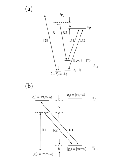
Figure 1: Relevant energy level structures for ${}^{9}\mathrm{Be}^{+}$ and ${}^{24}\mathrm{Mg}^{+}$ (not to scale) (a) Level structure for ${}^{9}\mathrm{Be}^{+}$. The ${}^{2}S_{1/2}$ levels are labelled by their $F$, $m_{F}$ quantum numbers. Beams D1, D2, and D3 are all polarized $\sigma^{-}$. Raman beams R1 and R2 are polarized $\pi$ and $\sigma^{+}/\sigma^{-}$ respectively with a detuning $\Delta\approx 2\pi\times 80\>\mathrm{GHz}$. For all beams $\lambda\simeq 313\;\mathrm{nm}.$ (b) Level structure for ${}^{24}\mathrm{Mg}^{+}$. Energy levels correspond to the $\left|J=\frac{1}{2},m_{J}=\pm\frac{1}{2}\right\rangle$ states. D1 is near resonant and polarized $\sigma^{-}$. Raman beams R1 and R2 are polarized $\pi$ and $\sigma^{+}/\sigma^{-}$ respectively, with a detuning $\Delta\approx 2\pi\times 750\>\mathrm{MHz}$. The $17\>\mathrm{G}$ field defining the quantization axis gives a ground state Zeeman splitting of $\delta\approx 2\pi\times 40\>\mathrm{MHz}$. For all beams $\lambda\approx 280\>\mathrm{nm}$.

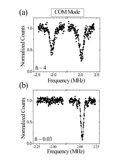
Figure 2: Results for the COM mode using ${}^{9}\mathrm{Be}^{+}$ as a cooling ion. Red (blue) sideband data is shown on the left (right). (a) Doppler cooling and (b) Sideband cooling. Values of $\bar{n}$ are estimated from the sideband ratio - see text.

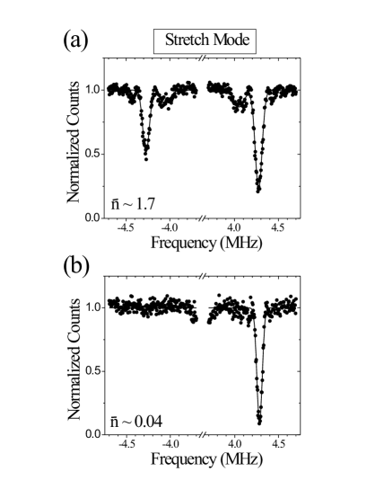
Figure 3: Results for the stretch mode using ${}^{9}\mathrm{Be}^{+}$ as a cooling ion. Red (blue) sideband data is shown on the left (right). (a) Doppler cooling and (b) Sideband cooling. Values of $\bar{n}$ are estimated from the sideband ratio - see text.

II.2 Magnesium Cooling

For ${}^{24}\mathrm{Mg}^{+}$ the relevant level structure is shown in Fig. 1(b). R2 is linearly polarized and propagates along the quantization axis giving equal contributions to its $\sigma^{+}/\sigma^{-}$ components. This choice, together with the $\pi$ polarized R1 beam, serves to partially balance the ac Stark shifts induced by the Raman beams . In addition, the intensity of the R1 beam is chosen so that it has the same coupling, $\Omega$ (Eq. (8)), to the excited states as the $\sigma$ components of the R2 beam. This choice gives the most favorable ratio of Raman coupling to spontaneous emission rate for this beam configuration. While a linearly polarized field tuned to the red of the ${}^{2}S_{1/2}\leftrightarrow\,^{2}P_{1/2}$ transition could provide Doppler cooling, this would require the use of an additional laser beam. To circumvent this need the initial Doppler cooling step is provided using ${}^{9}\mathrm{Be}^{+}$ as before. For sideband cooling, Raman transitions of a fixed duration are driven by beams R1 and R2, which are tuned to the $\left|g_{1},n\right\rangle\leftrightarrow\left|g_{2},n-1\right\rangle$ transition and oriented similarly to the Raman beams used for ${}^{9}\mathrm{Be}^{+}$. Each Raman pulse is then followed by an optical pumping pulse provided by the near resonant $\sigma^{-}$ polarized beam D1. Since the ${}^{2}S_{1/2}\leftrightarrow\,^{2}P_{1/2}$ manifold lacks a closed cycling transition, we use ${}^{9}\mathrm{Be}^{+}$ as before in order to probe the final ground state fraction and results are given in Fig. 4. From this data we infer a ground state occupancy of $0.84(4)$ for the COM mode and $0.66(3)$ for the stretch mode, with corresponding mean vibrational quanta of $\bar{n}=0.19(6)$ and $\bar{n}=0.52(7)$ respectively.

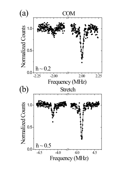
Figure 4: Cooling results using ${}^{24}\mathrm{Mg}^{+}$ as a cooling ion. Red (blue) sideband data is shown on the left (right). (a) COM mode and (b) Stretch mode. Values of $\bar{n}$ are estimated from the sideband ratio - see text.

The significant difference between the results obtained using ${}^{9}\mathrm{Be}^{+}$ as a refrigerant ion and those using ${}^{24}\mathrm{Mg}^{+}$ can be predominately attributed to spontaneous emission from the ${}^{24}\mathrm{Mg}^{+}$ Raman cooling beams. For ${}^{9}\mathrm{Be}^{+}$, the Raman beams are detuned by $\Delta\approx 2\pi\times 80\>\mathrm{GHz}$ and spontaneous emission plays a negligibly small role. However, for ${}^{24}\mathrm{Mg}^{+}$, all beams are derived from a single laser source with the Raman detuning achieved using acousto-optic modulators. As such our current setup limits the detuning of the Raman beams to $\Delta\approx 2\pi\times 750\>\mathrm{MHz}$, and this gives rise to a significant amount of spontaneous emission during a Raman cooling cycle. Specifically, one can show that the mean number of photons scattered in a time corresponding to a coherent $\pi$ pulse on the $\left|g_{1},n=1\right\rangle\leftrightarrow\left|g_{2},n=0\right\rangle$ transition is $0.55$ for the COM mode and $2.0$ for the stretch. With spontaneous emission, population cannot be completely transferred from one internal ground state to the other, and the ground state $\left|g_{1},n=0\right\rangle$ is no longer a dark state for the Raman cooling process. Thus, in any cooling cycle, population cannot be completely transferred to the vibrational ground state. Furthermore, after the Raman pulse, there will always be a finite amount of population left in the internal state, $\left|g_{2}\right\rangle$. This gives rise to a small amount of recoil heating during the final optical pumping step.

III Simulations

To more firmly establish spontaneous emission as the principal limitation when cooling with ${}^{24}\mathrm{Mg}^{+}$ we have used a master equation to model the cooling process, the details of which are given in the appendices. In these simulations we have used $\Omega=2\pi\times 30\>\mathrm{MHz}$, based on the measured beam intensities, which yields a carrier Rabi frequency associated with the Raman $\left|g_{1},n=0\right\rangle\leftrightarrow\left|g_{2},n=0\right\rangle$ transition of approximately $2\pi\times 300\>\mathrm{kHz}$. Raman pulse times of $2\>\mu\mathrm{s}$ and $5\>\mu\mathrm{s}$ were used, as in the experiments, for the COM and stretch mode respectively. The initial state was taken to be a thermal state in both cases with $\bar{n}=4$ for the COM and $\bar{n}=1.7$ for the stretch, consistent with the experimental data in Figs. 2(a) and  3(a).

The final distributions obtained from numerical integration of the master equation are given in Fig. 5. For these distributions we find ground state occupancies of $0.80$ for the COM mode and $0.77$ for the stretch mode with corresponding mean vibrational quanta of $\bar{n}=0.46$ and $\bar{n}=0.31$ respectively. These values of $\bar{n}$ are significantly different from those found in the experiment. However the distributions in Fig. 5 are not strictly thermal and are not well characterized by $\bar{n}$. Recall that we experimentally characterize the final state based on the measured sideband ratio and the assumption of a thermal state. Therefore, to make a better comparison to the experiment, we calculate the sideband ratios for the distributions in Fig. 5 and we find $r=0.18$ and $r=0.23$ for the COM and stretch respectively. These values, together with the assumption of a thermal distribution, give ground state occupancies of $0.82$ for the COM mode and $0.77$ for the stretch with corresponding mean vibrational quanta of $\bar{n}=0.23$ and $\bar{n}=0.30$ respectively. These values are in better agreement with experiment and, for comparison, we have included the estimated thermal distributions in Fig. 5.

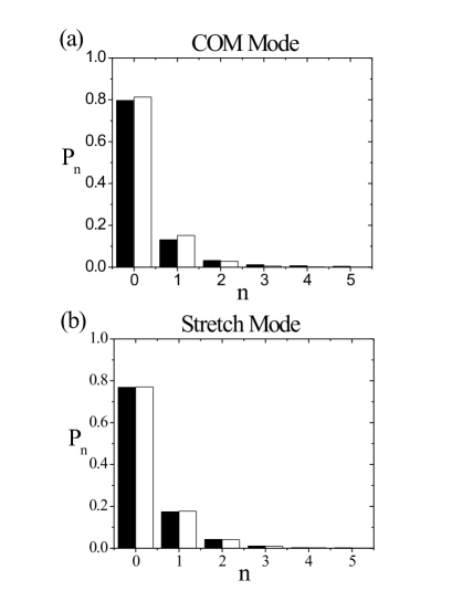
Figure 5: Simulation results using the master equation showing the final populations, $P_{n}$, vs. the respective vibrational quanta, $n$. (a) COM mode and (b) Stretch mode. Black bars correspond to the simulation results and the white bars are the estimated thermal distributions based on sideband ratios.

From the measured values of the frequencies and a normal mode analysis we calculate Lamb-Dicke parameters of $0.3$ for the COM mode and $0.082$ for the stretch. From these values, together with the carrier frequency quoted above, one might expect pulse times of $2.8\>\mu\mathrm{s}$ and $10\>\mu\mathrm{s}$ for the COM and stretch respectively based on calculated $\pi$ times for the $\left|g_{1},n=1\right\rangle\leftrightarrow\left|g_{2},n=0\right\rangle$ transition. The significant difference between these pulse times and those used in both the simulations and the experiments is due to that fact that we do not achieve ground state cooling. Thus the final optimum pulse need not be a $\pi$ pulse on $\left|g_{1},n=1\right\rangle\leftrightarrow\left|g_{2},n=0\right\rangle$ transition.

IV RF Micromotion Compensation

An additional technical advantage of using different atomic species arises from the difference in mass of the two ions. In a linear Paul trap Raizen et al. (1992); Wineland et al. (1998) the transversal confinement provided by the applied RF fields can be described by a harmonic pseudo-potential with a frequency that is inversely proportional to the mass of the ion. Thus, in the presence of a transverse stray electric field, the two ions have an equilibrium position that depends on the mass and their relative position vector no longer lies parallel to the trap axis. The net effect is that the modes are no longer separable into the axial and radial directions, and the measured frequencies deviate from those found in the absence of stray fields. Since this effect only occurs in the presence of stray fields, it provides an experimental method to detect and eliminate the RF-micromotion they induce.

To determine the effectiveness of this method we compare it with a previously demonstrated method in which the micromotion is monitored by measuring the below saturation scattering rate $R_{0}$ on the cycling transition in ${}^{9}\mathrm{Be}^{+}$ (D3 in Fig. 1(a)) when the laser is tuned near the carrier ($\omega_{\mathrm{laser}}-\omega_{\mathrm{atom}}\simeq 0$) and the scattering rate $R_{1}$ when the laser is tuned near the first micromotion-induced sideband ($\omega_{\mathrm{laser}}-\omega_{\mathrm{atom}}\simeq\pm\Omega_{RF}$) Berkeland et al. (1998). From these measurements the amplitude of the micromotion can be found from the ratio

$$R=\frac{R_{1}}{R_{0}}=\frac{J_{1}^{2}(\mathbf{k}\cdot\mathbf{u})}{J_{0}^{2}(\mathbf{k}\cdot\mathbf{u})}$$ (1)

where $J_{k}$ are Bessel functions of the first kind, $\mathbf{k}$ is the wave vector of the laser and $\mathbf{u}$ is the micromotion amplitude. To compare the two techniques we determine the effect on the frequency spectrum for a given $R$.

In the pseudo-potential approximation, the potential energy for a ${}^{9}\mathrm{Be}^{+}$ ion of mass $m$ can be written

$$V=\frac{m}{2}\bigg{[}\omega_{1}^{2}x_{1}^{2}+\left(\omega_{0}^{2}+\omega_{2}^{2}\right)x_{2}^{2}+\left(\omega_{0}^{2}-\omega_{3}^{2}\right)x_{3}^{2}\bigg{]},$$ (2)

where $\omega_{0}$ is the frequency associated with the RF pseudo-potential and $\omega_{1}^{2}$, $\omega_{2}^{2}$, and $-\omega_{3}^{2}$ are the curvatures associated with the applied static field needed to provide confinement along the trap axis $(\mathbf{\hat{x}}_{1})$ . Since $\omega_{0}$ and the static field curvatures $\omega_{k}^{2}$ are inversely proportional to the mass the potential energy of the two ion system can be written

$$V = \frac{m}{2}\bigg{[}\omega_{1}^{2}x_{1}^{2}+\left(\omega_{0}^{2}+\omega_{2}^{2}\right)x_{2}^{2}+\left(\omega_{0}^{2}-\omega_{3}^{2}\right)x_{3}^{2}\bigg{]}$$ (3)

$$+\frac{m}{2}\bigg{[}\omega_{1}^{2}y_{1}^{2}+\left(\mu^{-1}\omega_{0}^{2}+\omega_{2}^{2}\right)y_{2}^{2}$$

$$+\left(\mu^{-1}\omega_{0}^{2}-\omega_{3}^{2}\right)y_{3}^{2}\bigg{]}+\frac{q^{2}}{4\pi\epsilon_{0}}\frac{1}{|\mathbf{x}-\mathbf{y}|}$$

$$+am\omega_{0}^{2}\left[(x_{2}+y_{2})\cos{\theta}+(x_{3}+y_{3})\sin{\theta}\right],$$

where $\mathbf{x}$ and $\mathbf{y}$ denote the positions of ${}^{9}\mathrm{Be}^{+}$ and ${}^{24}\mathrm{Mg}^{+}$ respectively, $\mu$ is the ratio of the ${}^{24}\mathrm{Mg}^{+}$ mass to the ${}^{9}\mathrm{Be}^{+}$ mass, and $q$ is the ion’s charge. In this expression we have included a stray electric field

$$\mathbf{E}=a\frac{m\,\omega_{0}^{2}}{q}(\cos{\theta}\>\mathbf{\hat{x}}_{2}+\sin{\theta}\>\mathbf{\hat{x}}_{3}).$$ (4)

In the limit that $\omega_{0}$ dominates the radial confinement, $a$ is the off-axis displacement of ${}^{9}\mathrm{Be}^{+}$ due to the stray field. More generally it can be shown Berkeland et al. (1998) that an electric field of this form leads to micromotion of amplitude

$$\mathbf{u}=a\frac{\omega_{0}\sqrt{2}}{\Omega_{RF}}\left(\frac{\omega_{0}^{2}}{\omega_{0}^{2}+\omega_{2}^{2}}\cos{\theta}\>\mathbf{\hat{x}}_{2}+\frac{\omega_{0}^{2}}{\omega_{0}^{2}-\omega_{3}^{2}}\sin{\theta}\>\mathbf{\hat{x}}_{3}\right).$$ (5)

For our particular setup we have $\omega_{0}\simeq 2\pi\times 9\>\mathrm{MHz}$, $\omega_{1}\simeq 2\pi\times 2.8\>\mathrm{MHz}$, $\omega_{2}\simeq 2\pi\times 2\>\mathrm{MHz}$, and $\omega_{3}\simeq 2\pi\times 3.4\>\mathrm{MHz}$ and so we neglect the small dependence of the micromotion amplitude on the applied static field. If we assume a probe beam is optimally aligned for micromotion detection we have

$$\mathbf{k}\cdot\mathbf{u}=\frac{2\pi}{\lambda}\frac{\omega_{0}\sqrt{2}}{\Omega_{RF}}a.$$ (6)

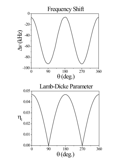
Figure 6: Plots showing effects of a transverse stray field on frequency spectrum for our experimental parameters. (a) Stretch mode shift and (b) Lamb-Dicke parameter for radial rocking mode in the $\mathbf{\hat{x}}_{2}$ as a function of the angle $\theta$.

Using this expression in Eq. (1) we can then find $a$ for a given ratio $R$. Using this value of $a$ in Eq. (3) we can find, for a given $\theta$, the equilibrium position and normal mode frequencies for the two ion system Goldstein (1981). In Fig. 6(a) we plot the shift in the stretch mode frequency as a function of $\theta$ using $R=0.1$ and the experimental value $\Omega_{RF}=2\pi\times 110\>\mathrm{MHz}$. The maximum frequency shift of $90\>\mathrm{kHz}$ is easily detected from the difference in the stretch mode sideband and carrier resonant frequencies. The minimum frequency shift of $7\>\mathrm{kHz}$ on the other hand would indicate a reduced sensitivity to stray fields acting along the $\hat{x}_{2}$ direction. The sensitivity could be increased by applying a static potential with negative curvature in this direction. This could be accomplished by, for example, applying an overall static potential difference between the RF and (RF grounded) control electrodes Rowe et al. (2002). Alternatively we could utilize an additional effect that influences the observed Raman frequency spectrum. The Raman beams used to probe the mode frequencies couple to all modes that have motion along the direction of the difference vector $\Delta\mathbf{k}=\mathbf{k}_{1}-\mathbf{k}_{2}$ which, in this case, is aligned along the trap axis. Thus, in the presence of a stray field, the Raman beams can couple to other modes giving rise to additional features in the frequency spectrum. The strength of this coupling is determined by the Lamb-Dicke parameter, $\eta_{1}$, and in Fig. 6(b) we plot the magnitude of $\eta_{1}$ as a function of $\theta$ for the radial rocking mode whose motion is nominally in the $\mathbf{\hat{x}}_{2}$ direction. The maximum value of $\eta_{1}\simeq 0.05$ gives rise to an easily detected feature in the frequency spectrum. Since this effect complements the shift of the stretch mode frequency, compensation of stray field from any direction can be accomplished.

Although the sensitivity of this approach depends on the strength of the RF confinement, it does have advantages over fluorescence measurements where, to null micromotion in the transverse direction, we require two non-parallel probe laser beam directions. In particular, monitoring the motional frequency spectrum does not require any additional optical access and is sensitive to micromotion in all transverse directions. Furthermore, the mode frequencies are needed for quantum logic experiments anyway and so monitoring the spectrum is a natural part of the experiment setup. As such, we have found this property to be a convenient method to detect and compensate the presence of stray fields.

V Spontaneous Emission and Stark Shifts

The advantage of using a different atomic species for the refrigerant ion is in the small Stark shifts and off-resonant excitation of the qubit ion due to the presence of the cooling light. Although the spontaneous emission and Stark shifts on the qubit ion will depend on the exact experimental conditions, we can get an estimate of these effects with the following simple model. We calculate the probability of spontaneous emission from a qubit based on a superposition of the $|\!\downarrow\rangle$ and $|\!\uparrow\rangle$ states of ${}^{9}\mathrm{Be}^{+}$, during a $\pi$ pulse on the $|g_{1},n=1\rangle\leftrightarrow|g_{2},n=0\rangle$ ${}^{24}\mathrm{Mg}^{+}$ Raman cooling transition. (This will be the dominant source of spontaneous emission during one cooling cycle since the re-pumping pulse is assumed to be near resonant and therefore of much less intensity.) We assume the laser beam intensity is the same on both ions. The time for the cooling pulse is given by $\tau_{\pi}\simeq 2\pi\Delta/(\eta\Omega^{2})$. From Ref. Wineland et al. (2002a), we find the rate of spontaneous emission from the ⁹Be⁺ qubit to be $R_{SE}=(3/2)\gamma\Omega^{2}/(\Delta^{*})^{2}$ where $\Delta^{*}$ is the frequency difference between the relevant transitions for ⁹Be⁺ and ²⁴Mg⁺. Therefore, the probability of spontaneous emission from the qubit superposition is given by $P_{SE}=R_{SE}\tau_{\pi}=3\pi\gamma\Delta/(\eta(\Delta^{*})^{2})$. For the COM mode ($\eta=0.3$), using the experimental values from Sec. III, we find $P_{SE}\simeq 4\times 10^{-11}$. Better cooling with ${}^{24}\mathrm{Mg}^{+}$ does require us to increase the Raman beam detuning, which leads to a corresponding increase in the probability of spontaneous emission (proportional to $\Delta$), but this should still yield a negligible probability of spontaneous emission.

To estimate Stark shifts on the qubit, we first note that by using linearly polarized light to drive the ${}^{24}\mathrm{Mg}^{+}$ Raman cooling transition, net Stark shifts on the ${}^{9}\mathrm{Be}^{+}$ qubit will vanish Wineland et al. (2002a). However, during the ${}^{24}\mathrm{Mg}^{+}$ re-pumping pulse, we require $\sigma^{+}$ light, which leads to Stark shifts on the qubit. From Ref. Wineland et al. (2002a), we estimate the phase shift on the qubit for each re-pumping pulse to be approximately $\Delta\phi\simeq 3\times 10^{-10}$. Because the expected decoherence from spontaneous emission and Stark shifts are so small, we could not test these predictions. Nevertheless, we did look for decoherence due to presence of the ${}^{24}\mathrm{Mg}^{+}$ Raman cooling beams. We performed a Ramsey resonance experiment on the $|\downarrow\rangle\rightarrow|\uparrow\rangle$ transition in ${}^{9}\mathrm{Be}^{+}$ with a precession time of 10 ms and observed no loss in contrast ($5\%$ accuracy) with the ${}^{24}\mathrm{Mg}^{+}$ Raman beams applied continuously with maximum intensity during this time.

VI Conclusion

We have demonstrated sympathetic cooling of a two ion crystal consisting of one ${}^{9}\mathrm{Be}^{+}$ and one ${}^{24}\mathrm{Mg}^{+}$. Using ${}^{9}\mathrm{Be}^{+}$ as the cooling ion, we have been able to achieve a ground state occupancy for the axial modes of $\sim 95\%$ and better cooling results can be expected with improvements in the apparatus. With ${}^{24}\mathrm{Mg}^{+}$ as the cooling ion we are currently limited by spontaneous emission. A model has been developed which takes spontaneous emission into account and gives reasonable agreement with the experimental results. Thus, for ${}^{24}\mathrm{Mg}^{+}$ cooling, we expect to find a substantial improvement in the cooling results when we use larger detunings. For the purposes of quantum information processing one can anticipate the need to cool more than two ions: the three ion crystal consisting of two qubits and one refrigerant being an obvious example. For such cases the salient features of the cooling process are essentially the same as those demonstrated here, provided the normal mode frequencies can be spectrally resolved. This spectral resolution will typically be achievable in the case where two adjacent qubit ions are cooled by a third refrigerant ion Wineland et al. (1998); Kielpinski et al. (2002). A configuration where an even number of qubit ions is cooled by a centrally located refrigerant ion Kielpinski et al. (2002) should also be experimentally feasible. Finally, we note that these techniques may find use outside the realm of quantum computation, for instance, when applied to atomic clocks Wineland et al. (2002b).

In addition to demonstrating sympathetic cooling, we have found that a mass difference between ions gives rise to a novel technique to detect and eliminate the effects of RF micromotion. This technique involves monitoring the motional frequency spectrum only and, as such, it is a very convenient and easily implemented method of micromotion compensation.

The authors thank Marie Jensen and Piet O. Schmidt for suggestions and comments on the manuscript. This work was supported by the U.S. National Security Agency (NSA) and Advanced Research and Development Activity (ARDA) under contract No. MOD-7171.00, the U.S. Office of Naval Research (ONR), and the National Institute of Standards and Technology (NIST), an agency of the U.S. government. This paper is a contribution of NIST and is not subject to U.S. copyright.

Appendix A Model

In the interaction picture the master equation has the usual form

$$\dot{\rho}=-i\left[H_{I},\rho\right]+L\rho$$ (7)

where $H_{I}$ is the interaction Hamiltonian and $L$ is the Liouvillian operator which accounts for dissipative processes. For the ${}^{24}\mathrm{Mg}^{+}$ system depicted in Fig. 1(b) the Hamiltonian is given by

$$H_{I} = \frac{\Omega}{2}\,e^{i\Delta t}\bigg{[}D\left(e^{i\delta_{L}t}\left|e_{1}\right\rangle\left\langle g_{1}\right|+e^{i(\delta_{L}-\frac{2}{3}\delta)t}\left|e_{2}\right\rangle\left\langle g_{2}\right|\right)$$ (8)

$$+D^{{\dagger}}\left(\left|e_{1}\right\rangle\left\langle g_{2}\right|+e^{i\frac{4}{3}\delta t}\left|e_{2}\right\rangle\left\langle g_{1}\right|\right)\bigg{]}+c.c.$$

where $\delta_{L}=\omega_{R2}-\omega_{R1}-\delta$ is the relative detuning of the Raman beams from the Raman resonance and $D$ is the kick or recoil operator. In terms of the annihilation operator, $a$, the normal mode frequency, $\omega$, and the corresponding Lamb-Dicke parameter, $\eta$, this operator may be written

$$D=\exp\left[i\frac{\eta}{2}\left(ae^{-i\omega t}+a^{{\dagger}}e^{i\omega t}\right)\right].$$ (9)

where we have restricted our attention to the mode of interest and $\eta$ is defined in terms of $\Delta\mathbf{k}$ for the Raman beams. Using the notation $\sigma_{jk}=\left|g_{j}\right\rangle\left\langle e_{k}\right|$ the Liouvillian has the usual form

$$L\rho=\frac{\Gamma}{2}\sum\limits_{j,k}c_{jk}^{2}(2\sigma_{jk}\bar{\rho}\sigma_{jk}^{{\dagger}}-\sigma_{jk}^{{\dagger}}\sigma_{jk}\rho-\rho\sigma_{jk}^{{\dagger}}\sigma_{jk})$$ (10)

where $c_{jk}$ is the Clebsch-Gordon coefficient connecting $\left|g_{j}\right\rangle$ and $\left|e_{k}\right\rangle$, $\Gamma$ is the total decay rate from the excited state, and $\bar{\rho}$ describes the density matrix after a spontaneous emission event Cirac et al. (1994); Javanainen and Stenholm (1980):

$$\bar{\rho} = \iint d\,\Omega\,W(\hat{k}\cdot\hat{e}_{z})\exp\left(i\eta\frac{\hat{k}\cdot\hat{e}_{t}}{\sqrt{2}}\left(ae^{-i\omega t}+a^{{\dagger}}e^{i\omega t}\right)\right)$$ (11)

$$\times\rho\exp\left(-i\eta\frac{\hat{k}\cdot\hat{e}_{t}}{\sqrt{2}}\left(ae^{-i\omega t}+a^{+}e^{i\omega t}\right)\right).$$

In this expression $\hat{k}$ is the unit vector giving the propagation direction of the scattered photon relative to the quantization axis denoted $\hat{e}_{z}$, $\hat{e}_{t}$ is a unit vector along the trap axis, $W(\hat{k}\cdot\hat{e}_{z})$ is the angular distribution of the emission, and the integration is carried over the full solid angle. For the dipole decay discussed here we have

$$W(\hat{k}\cdot\hat{e}_{z})=\frac{3}{8\pi}\begin{cases}\left(1-(\hat{k}\cdot\hat{e}_{z})^{2}\right),\\ \frac{1}{2}\left(1+(\hat{k}\cdot\hat{e}_{z})^{2}\right)\end{cases}$$ (12)

where the upper (lower) expression applies to decay channels involving linear (circular) polarization.

Appendix B Adiabatic Elimination

The master equation formulated in appendix A can be integrated directly using a truncated basis of Fock states to describe the vibrational modes. However it is computationally intensive to do so and significant simplification can be achieved by adiabatically eliminating the excited state. The procedure we adopt here closely follows that found in Dalibard et al. (1992).

Let $P_{g}$ and $P_{e}$ be the projection operators defined by $P_{g}=\sum\limits_{k}\left|g_{k}\right\rangle\left\langle g_{k}\right|$ and $P_{e}=\sum\limits_{k}\left|e_{k}\right\rangle\left\langle e_{k}\right|$. Then any operator, $A$, can be written as $A=A_{ee}+A_{eg}+A_{ge}+A_{gg}$ where $A_{ab}=P_{a}AP_{b}$. In this way the master Eq. (7) can be rewritten in component form giving

$$\dot{\rho}_{ee} = -i\left(\tilde{H}_{eg}\tilde{\rho}_{ge}-\tilde{\rho}_{eg}\tilde{H}_{ge}\right)-\Gamma\rho_{ee}$$ (13)

$$\dot{\tilde{\rho}}_{eg} = -i\left(\tilde{H}_{eg}\rho_{gg}-\rho_{ee}\tilde{H}_{eg}\right)-\left(\frac{\Gamma}{2}+i\Delta\right)\tilde{\rho}_{eg}$$ (14)

$$\dot{\rho}_{gg} = -i\left(\tilde{H}_{ge}\tilde{\rho}_{eg}-\tilde{\rho}_{ge}\tilde{H}_{eg}\right)$$ (15)

$$\qquad+\Gamma\sum\limits_{j,k}c_{jk}^{2}\sigma_{jk}\bar{\rho}_{ee}\sigma_{jk}^{+},$$

where have used the definitions $H_{I}=e^{i\Delta t}\tilde{H}_{eg}+c.c$ and $\tilde{\rho}_{eg}=e^{-i\Delta t}\rho_{eg}.$ To proceed we neglect the the terms $\dot{\tilde{\rho}}_{eg}$ and $\rho_{ee}\tilde{H}_{eg}$ in Eq. (14), the validity of which is discussed in Dalibard et al. (1992). This results in an algebraic expression for $\tilde{\rho}_{eg}$ which can be rearranged to give

$$\tilde{\rho}_{eg}=\frac{-i}{(\Gamma/2)+i\Delta}\tilde{H}_{eg}\rho_{gg}.$$ (16)

Substituting this expression into Eq. (13) and neglecting $\dot{\rho}_{ee}$ then yields the result

$$\rho_{ee}=\frac{1}{(\Gamma/2)^{2}+\Delta^{2}}\tilde{H}_{eg}\rho_{gg}\tilde{H}_{ge}.$$ (17)

Finally, Eqs. (16) and (17) can be substituted into Eq. (15) to give a closed equation of motion for $\rho_{gg}$. Dropping the subscripts on $\rho_{gg}$ we find the equation

$$\dot{\rho} = -i\left[\frac{-\Delta}{(\Gamma/2)^{2}+\Delta^{2}}\tilde{H}_{ge}\tilde{H}_{eg},\rho\right]-\left\{\frac{(\Gamma/2)}{(\Gamma/2)^{2}+\Delta^{2}}\tilde{H}_{ge}\tilde{H}_{eg},\rho\right\}+\frac{(\Gamma/2)}{(\Gamma/2)^{2}+\Delta^{2}}\sum\limits_{j,k}c_{jk}^{2}2\sigma_{jk}\tilde{H}_{eg}\bar{\rho}\tilde{H}_{ge}\sigma_{jk}^{{\dagger}}$$ (18)

for the effective ground state density matrix, where $\{\>,\}$ is used to denote an anti-commutator. If one makes the identifications

$$H_{\mathrm{\textit{eff}}} =\frac{-\Delta}{(\Gamma/2)^{2}+\Delta^{2}}\tilde{H}_{ge}\tilde{H}_{eg},$$

$$\Gamma^{\prime} =\frac{\Gamma}{(\Gamma/2)^{2}+\Delta^{2}},$$

and

$$\bar{\sigma}_{jk} =\sigma_{jk}\tilde{H}_{eg}$$

then Eq. (18) can be recast into the usual form given in Eqs. (7) and (10). Numerical simulation of the reduced master equation can be further simplified by expanding out the terms in (18) and neglecting the off-resonant terms associated with the Raman pair $\sigma^{+}$ and $\pi$.

The resulting system gives excellent agreement with the full system given in Eq. (7). However the procedure outlined here is not rigorously correct due the residual time-dependence in $\tilde{H}_{eg}$ associated with the Zeeman splitting of the excited and ground state manifolds. In effect, the procedure here neglects the small differential Stark shift induced by this splitting as well as the small change in the various spontaneous emission rates. These have been accounted for in a more elaborate treatment in which the projection operators are split allowing the individual level shifts to be accounted for. The resulting algebra is more involved but the procedure is precisely the same. For brevity and clarity we have omitted the details of this more elaborate treatment. Finally, we note that the optical pumping process can be treated in a similar manner with Eq. (8) replaced with

$$H_{I}=\frac{\Omega}{2}D^{{\dagger}}\left|e_{1}\right\rangle\left\langle g_{2}\right|+c.c.$$ (19)

References

- Cirac and Zoller (1995) J. I. Cirac and P. Zoller, Phys. Rev. Lett. 74, 4091 (1995).
- Schmidt-Kaler et al. (2003) F. Schmidt-Kaler et al., Nature 422, 408 (2003).
- Sørensen and Mølmer (1999) A. Sørensen and K. Mølmer, Phys. Rev. Lett. 82, 1971 (1999).
- Sørensen and Mølmer (2000) A. Sørensen and K. Mølmer, Phys. Rev. A 62, 022311 (2000).
- Milburn et al. (2000) G. J. Milburn, S. Schneider, and D. F. V. James, Fortschritte der Physik 48, 801 (2000).
- Cirac and Zoller (2000) J. I. Cirac and P. Zoller, Nature 404, 579 (2000).
- Calaraco et al. (2001) T. Calaraco, J. I. Cirac, and P. Zoller, Phys. Rev. A 63, 062304 (2001).
- James (2000) D. F. V. James, in Scalable Quantum Computers, edited by S. L. Braunstein, H. K. Lo, and P. Kok (Wiley-VCH, Berlin, 2000), pp. 53–68.
- Sackett et al. (2000) C. A. Sackett et al., Nature 404, 256 (2000).
- Leibfried et al. (2003) D. Leibfried et al., Nature 422, 412 (2003).
- Wineland et al. (1998) D. J. Wineland et al., J. Res. Natl. Inst. Stand. Technol. 103, 259 (1998).
- Kielpinski et al. (2002) D. Kielpinski, C. Monroe, and D. J. Wineland, Nature 417, 709 (2002).
- Rowe et al. (2002) M. A. Rowe et al., Quant. Inf. and Comp. 2, 257 (2002).
- Larson et al. (1986) D. J. Larson et al., Phys. Rev. Lett. 57, 70 (1986).
- Rohde et al. (2001) H. Rohde et al., J. Opt. B. 3, S34 (2001).
- Steane et al. (2000) A. Steane et al., Phys. Rev. A 62, 042305 (2000).
- Blinov et al. (2002) B. B. Blinov, L. Deslauriers, P. Lee, M. J. Madsen, R. Miller, and C. Monroe, Phys. Rev. A 65, 040304 (2002).
- Kelpinski et al. (2000) D. Kelpinski et al., Phys. Rev. A 61, 032310 (2000).
- Morigi and Walter (2001) G. Morigi and H. Walter, Eur. Phys. J. D 13, 261 (2001).
- Wineland and Itano (1979) D. J. Wineland and W. M. Itano, Phys. Rev. A 20, 1521 (1979).
- Metcalf and van der Straten (1999) H. J. Metcalf and P. van der Straten, Laser Cooling and Trapping (Springer, 1999).
- Monroe et al. (1995) C. Monroe et al., Phys. Rev. Lett. 75, 4011 (1995).
- Turchette et al. (2000) Q. A. Turchette et al., Phys. Rev. A 61, 063418 (2000).
- Raizen et al. (1992) M. G. Raizen, J. M. Gilligan, J. C. Berquist, W. M. Itano, and D. J. Wineland, Phys. Rev. A 45, 6493 (1992), and references therein.
- Berkeland et al. (1998) D. J. Berkeland, D. J. Miller, J. C. Bergquist, W. M. Itano, and D. J. Wineland, J. Appl. Phys. 83, 5025 (1998).
- Goldstein (1981) H. Goldstein, Classical Mechanics (Addison-Wesley, 1981), 2nd ed.
- Wineland et al. (2002a) D. J. Wineland et al. (2002a), eprint quant-ph/0212079.
- Wineland et al. (2002b) D. J. Wineland, J. C. Bergquist, J. J. Bollinger, R. E. Drullinger, and W. M. Itano, in Proc. 6th Symposium Frequency Standards and Metrology, edited by P. Gill (World Scientific, Singapore, 2002b), pp. 361–368.
- Cirac et al. (1994) J. I. Cirac, L. J. Garay, R. Blatt, A. S. Parkins, and P. Zoller, Phys. Rev. A 49, 421 (1994).
- Javanainen and Stenholm (1980) J. Javanainen and S. Stenholm, Appl. Phys. 21, 35 (1980).
- Dalibard et al. (1992) J. Dalibard, J.-M. Raimond, and J. Zinn-Justin, eds., Fundamental systems in quantum optics (North-Holland, 1992), course I.