Numerical analysis of a spontaneous collapse model for a two–level system

Abstract

We study a spontaneous collapse model for a two–level (spin) system, in which the Hamiltonian and the stochastic terms do not commute. The numerical solution of the equations of motions allows to give precise estimates on the regime at which the collapse of the state vector occurs, the reduction and delocalization times, and the reduction probabilities; it also allows to quantify the effect that an Hamiltonian which does not commute with the reducing terms has on the collapse mechanism. We also give a clear picture of the transition from the “microscopic” regime (when the noise terms are weak and the Hamiltonian prevents the state vector to collapse) to the “macroscopic” regime (when the noise terms are dominant and the collapse becomes effective for very long times). Finally, we clarify the distinction between decoherence and collapse.

I Introduction

Stochastic Schrödinger equations find fruitful applications both in the theory of open quantum systems da ; lib ; pk ; bas ; peo and within collapse models gpr ; per ; pp ; di ; bel ; bar ; bla ; jp ; ip ; ad1 ; ad2 ; rep . In the first case, the stochastic terms mimic the effect of the environment on the open system. In the second case, non–linear and stochastic terms are added to the standard Schrödinger equation to reproduce — under appropriate conditions — the collapse of the wavefunction; in this way, it is possible to describe within one single dynamical equation both the quantum properties of microscopic systems and the classical properties of macroscopic objects, and in particular the outcomes of measurement processes.

In this paper, we analyze with numerical techniques the dynamics described by the following stochastic Schrödinger equation in the Hilbert space ${\mathbb{C}}^{2}$:

$$d|\psi_{t}\rangle = \left[-i\omega\sigma_{x}dt\,+\,\sqrt{\gamma}(\sigma_{z}-\langle\sigma_{z}\rangle)\,dW_{t}\frac{}{}\right.$$ (1)

$$\left.-\frac{\gamma}{2}(\sigma_{z}-\langle\sigma_{z}\rangle)^{2}\,dt\,\right]|\psi_{t}\rangle,$$

which is nonlinear and, as a consequence, nonunitary; anyway, it is easy to check that it preserves the norm of $|\psi_{t}\rangle$. $\langle\sigma_{z}\rangle$ denotes the quantum average $\langle\psi_{t}|\sigma_{z}|\psi_{t}\rangle$, while $\sigma_{x}$, $\sigma_{z}$ are the usual spin operators. $W_{t}$ is a standard Wiener process: ${\mathbb{E}}\,[dW_{t}]=0$ and ${\mathbb{E}}\,[dW_{t}^{2}]=dt$, and the (positive) parameter $\gamma$ measures the strength of the coupling between the spin operator $\sigma_{z}$ and $W_{t}$. Finally, the stochastic dynamics is defined on a probability space $(\Omega,{\mathcal{F}},{\mathbb{P}})$ with the filtration $\{{\mathcal{F}}_{t}:t\in[0,\infty)\}$ generated in a standard way by the Wiener process $W_{t}$.

Eq. (1) describes the evolution of the spin–wavefunction of a $1/2$ spin particle; the dynamics is non–trivial, due to the presence of two competing terms which do not commute: on the one side the Hamiltonian $H=\hbar\omega\sigma_{x}$, whose effect is to rotate the state vector along the $x$ axis of the Bloch sphere; on the other side, the spin operator $\sigma_{z}$ which tends to localize the state vector along one of its two eigenstates $|+\rangle$, $|-\rangle$.

We will begin our analysis by studying the equation for the statistical operator $\rho(t)$ — describing the ensemble of states each of which evolves according to Eq. (1) — which in this case can be solved exactly (section II); we will give a qualitative description of the evolution of $|\psi_{t}\rangle$, based on the dynamics for $\rho(t)$. We will next solve Eq. (1) numerically, showing that a much richer quantity of information can be obtained: in particular, we will analyze the regime in which the reduction of the state vector to one of the two eigenstates of $\sigma_{z}$ occurs, and we will clarify the distinction between collapse and decoherence (section III); we will analyze the reduction probabilities (section IV), the delocalization mechanism (section V), and the transition from the “quantum” ($\gamma\ll\omega$) to the “classical” ($\gamma\gg\omega$) regime (section VI). We will conclude our analysis with a comparison between the model here analyzed and space–collapse models (section VII).

II The statistical operator

The statistical operator $\rho(t)={\mathbb{E}}\,[|\psi_{t}\rangle\langle\psi_{t}|]$ obeys the equation of motion:

$$\frac{d}{dt}\,\rho(t)\;=\;-i\omega\,\left[\sigma_{x},\rho(t)\right]\,-\,\gamma\left[\rho(t)-\sigma_{z}\rho(t)\sigma_{z}\right],$$ (2)

which of course is of the Lindblad–type lind . It can be solved analytically for any given initial condition; if we consider the matrix elements of $\rho$ with respect to the eigenstates $|+\rangle$, $|-\rangle$ of $\sigma_{z}$:

$$\rho\;\longrightarrow\;\left(\begin{array}[]{cc}\langle+|\rho|+\rangle&\langle+|\rho|-\rangle\\ \langle-|\rho|+\rangle&\langle-|\rho|-\rangle\end{array}\right)\;=\;\left(\begin{array}[]{cc}x&y+iz\\ y-iz&1-x\end{array}\right),$$

we get the following equations for $x$, $y$ and $z$:

$$\left\{\begin{array}[]{lll}\dot{x}(t)&=&-2\omega\,z(t)\\ \dot{y}(t)&=&-2\gamma\,y(t)\\ \dot{z}(t)&=&-\omega+2\omega\,x(t)-2\gamma\,z(t).\end{array}\right.$$ (3)

The complete solutions of equations (3) are written in appendix I; here we limit ourselves to discuss some general features.

The equation for $y(t)$ is, trivially, a decaying exponential; the two equations for $x(t)$ and $z(t)$ lead to the following second–order differential equation for $z(t)$:

$$\ddot{z}(t)\;+\;2\gamma\,\dot{z}(t)\;+\;4\omega^{2}\,z(t)\;=\;0,$$ (4)

which is the equation of a damped harmonic oscillator; accordingly, for any value of $\omega$ and $\gamma$ (different from zero) the off–diagonal elements of the density matrix decrease exponentially in time. This results would suggest that reductions occur for any value of $\gamma$ — even though, of course, we expect the localization mechanism to be less efficient for smaller values of $\gamma$ — but we will see in the following sections that the real situation is subtler.

The time evolution of $x(t)$ has the following interesting property: for any value of $\omega$ and $\gamma$ (different from zero) and for any given initial condition, one has

$$x(t)\xrightarrow[t\,\rightarrow\,+\infty]{}\frac{1}{2}$$ (5)

This result is interpreted in the following way: suppose that the initial (at time $t=0$) state vector is, e.g.:

$$|\psi_{0}\rangle\;=\;\sqrt{\frac{3}{4}}\,|+\rangle\;+\;\sqrt{\frac{1}{4}}\,|-\rangle,$$ (6)

and assume that after a certain amount of time it has been stochastically reduced either to the state $|+\rangle$ or to the state $|-\rangle$, with the correct quantum probabilities. As a consequence, the density matrix becomes almost diagonal, with the diagonal elements equal to $3/4$ and $1/4$.

Result (5) states that, as time goes to infinity, the diagonal elements must change and become asymptotically equal to $1/2$: this implies that, however it has been initially reduced, the state vector starts jumping between the two eigenstates, so that after a certain amount of time there is an equal probability of finding it either reduced around $|+\rangle$ or around $|-\rangle$, despite that, at the very beginning, there was a much higher probability to find it reduced around $|+\rangle$. In the following sections we will give a quantitative analysis of this effect.

Note that the above result does not come as a surprise, since a general theorem by Spohn sp assures that, in the finite–dimensional case, when an equation of the quantum dynamical semigroup type admits a steady solution, then any other solution converges to it for $t\,\rightarrow\,+\infty$. In our case, equation (2) has $\frac{1}{2}I$ as the only steady solution, where $I$ is the identity matrix: accordingly, the off–diagonal elements must necessarily vanish as time increases, while the diagonal elements must converge to $1/2$.

III Reduction times

The dynamics described by eq. (1) has several interesting properties. The first quantity which we have analyzed is the reduction time, i.e. the time it takes for the state vector to reduce to one of the two eigenstates $|+\rangle$, $|-\rangle$ of the spin operator $\sigma_{z}$. A reduction process must satisfy the following two requirements:

1. The state vector $|\psi_{t}\rangle$ must get “close enough” to one of the eigenstates of the reducing operator, $\sigma_{z}$ in our case;

2. Once the state vector reaches such an eigenstate, it must remain close to it for a “sufficiently long” time interval.

Let us make these two requirements more precise. When $|\psi_{t}\rangle$ gets close to the eigenstate $|+\rangle$ ($|-\rangle$), the square modulus $|\langle+|\psi_{t}\rangle|^{2}$ (respectively, $|\langle-|\psi_{t}\rangle|^{2}$) approaches the value 1: accordingly, the first requirement amounts to saying that either $|\langle+|\psi_{t}\rangle|^{2}$ or $|\langle-|\psi_{t}\rangle|^{2}$ is greater than $1-\varepsilon$, where $\varepsilon$ is a parameter depending on the physical situation under study. Following the second requirement, when — let us say — it happens that $|\langle+|\psi_{t}\rangle|^{2}>1-\varepsilon$, a reduction has occurred only if this condition holds for a time interval of length $\tau$; once more, the suitable value for $\tau$ depends on the specific physical system.

According to the above arguments, we define the reduction time as follows: it is the smallest time $t_{r}$ such that, for $t\in[t_{r},t_{r}+\tau]$, the square modulus $|\langle+|\psi_{t}\rangle|^{2}$ (or $|\langle-|\psi_{t}\rangle|^{2}$) is greater than $1-\varepsilon$.

Fig. 1 shows the results of the numerical simulations for the reduction time as a function of $\gamma$, with the initial state vector $|\psi_{0}\rangle$ as in eq. (6) and $\omega=1$ s^-1.

Figure 1: Reduction time $t_{r}$ as a function of $\gamma$; the simulations have been made for $\gamma=5,10,20,40,60,80,100$ s^-1, while $\omega=1$ s^-1. The picture shows the average values and the standard deviations over 100000 trajectories. Above each bar, we have indicated the fraction of the total trajectories which have been reduced within the time interval $[0,2\pi]$ seconds.

We have taken $\varepsilon=1/100$, while $\tau$ has been chosen according to the following criterion: when $\gamma=0$ and $|\psi_{0}\rangle=|+\rangle$ or $|-\rangle$, the state vector rotates between the two eigenstates of $\sigma_{z}$ with frequency $\omega$. Accordingly, even if no reducing terms are present, the dynamics brings periodically $|\psi_{t}\rangle$ close to, e.g., $|+\rangle$, in such a way that $|\langle+|\psi_{t}\rangle|^{2}$ remains greater than $1-\varepsilon$ for a time equal to: $\pi/2-\arcsin(1-\varepsilon)\simeq 0.141$ s. We have then chosen $\tau$ to be equal to $10\times[\pi/2-\arcsin(1-\varepsilon)]$, to distinguish a reduction from the effects of the oscillatory motion induced by the Hamiltonian $H$.

The simulation shows that, as expected, the reduction time decreases for increasing values of $\gamma$. When $\gamma$ is sufficiently larger than $\omega$ ($\gamma\geq 60$ s^-1), the reduction time becomes a well–defined quantity: all trajectories are reduced, and the variance associated to $t_{r}$ decreases as $\gamma$ increases. On the other hand, when $\gamma$ is of the same order of — or smaller than — $\omega$, only a few trajectories (or none) are localized and the variance associated to the reduction times, increases: in this regime, the reduction process progressively disappears. This result is particularly important in relation to the time evolution of the off–diagonal elements of the density matrix.

In the previous section, we have seen that, for any value of $\gamma$, the off–diagonal elements of the density matrix decrease exponentially in time. According to the numerical simulations of Fig. 1, such a damping has two different origins according to whether $\gamma$ is significantly greater than $\omega$ or not: in the first case, the damping is due to the localization process; in the second case, it is a consequence of a phase randomization (decoherence) of the different trajectories.

This property of eq. (1) is well represented in Figs. 2 and 3.

Figure 2: a) Time evolution of the real (dotted line) and imaginary (continuous line) parts of $\langle+|\psi_{t}\rangle\langle\psi_{t}|-\rangle$, for a typical trajectory followed by the state vector. The parameter $\gamma$ has been taken equal to $0.05$ s^-1, while as usual $\omega=1$ s^-1. b) and c) show the average values over 5 and 100 different trajectories, respectively. Note the decoherence effect: as time increases, the imaginary parts pick up different random phases and interfere destructively. d) shows the (theoretical) average values, corresponding to the time evolution of the real ($y$) and imaginary ($z$) parts of the off–diagonal element $\langle+|\rho(t)|-\rangle$ of the density matrix.

Figure 3: As in Fig. 2, but with $\gamma=50$ s^-1. Only the imaginary parts can be seen, as the real ones go rapidly to zero. Note that the decoherence effect is almost absent: when $\gamma$ is sufficiently larger than $\omega$, single trajectories share the property that both the real and the imaginary parts of $\langle+|\psi_{t}\rangle\langle\psi_{t}|-\rangle$ are (most of the time) close to zero.

Fig. 2a shows a typical trajectory for the real and imaginary parts of $\langle+|\psi_{t}\rangle\langle\psi_{t}|-\rangle$, when $\gamma=0.05$ s^-1: the real part (dotted line) decreases in time, while the imaginary part (continuous line) oscillates and does not approach the value zero. Figs. 2b and 2c show the average values over 5 and 100 trials, respectively; while the time evolution of the real part of $\langle+|\psi_{t}\rangle\langle\psi_{t}|-\rangle$ does not change in a significant way, the evolution of the imaginary part displays a typical decoherence effect: the trajectories pick up different random phases and interfere destructively. Decoherence is then responsible of the exponential damping of the off–diagonal element $\langle+|\rho(t)|-\rangle={\mathbb{E}}\,[\langle+|\psi_{t}\rangle\langle\psi_{t}|-\rangle]$ of the statistical operator, as shown in Fig. 2d.

Fig. 3a, instead, shows the result of the numerical simulations for the (typical) evolution of the real and imaginary parts of $\langle+|\psi_{t}\rangle\langle\psi_{t}|-\rangle$, when $\gamma=50$ s^-1: both parts are almost always close zero, as an effect of the reduction process. Figs. 3b and 3c show an average over 5 and 100 trials respectively, while Fig. 3d shows the mean value $\langle+|\rho(t)|-\rangle={\mathbb{E}}\,[\langle+|\psi_{t}\rangle\langle\psi_{t}|-\rangle]$: in this regime, the damping of the off–diagonal elements of the density matrix is not due to a decoherence effect but to the reduction process, since (almost all) realizations of $\langle+|\psi_{t}\rangle\langle\psi_{t}|-\rangle$ are vanishingly small.

IV Probabilities

The second interesting quantity to analyze is the probability that the state vector reduces toward either the eigenstate $|+\rangle$ or the eigenstate $|-\rangle$. The results of the simulation are shown in table 1. When $\gamma$ is much larger than $\omega$, the probability that a reduction occurs approaches the quantum probabilities of finding the value $+1$ or $-1$ in a measurement of the observable $\sigma_{z}$, given the initial state vector (6):

Prob.[reduction near $$|+\rangle \simeq |\langle+|\psi_{0}\rangle|^{2}\;=\;3/4$$]

Prob.[reduction near $$|-\rangle \simeq |\langle+|\psi_{0}\rangle|^{2}\;=\;1/4$$]

$\gamma$ (s-1)	red. near $|+\rangle$	red. near $|-\rangle$	total red.
100	73879 (74%)	26121 (26%)	100000 (100%)
80	74076 (74%)	25924 (26%)	100000 (100%)
60	73748 (74%)	26252 (26%)	100000 (100%)
40	73142 (73%)	26858 (27%)	100000 (100%)
20	70411 (71%)	29033 (29%)	99444 (99%)
10	45862 (66%)	23279 (34%)	69141 (69%)
5	3432 (61%)	2165 (39%)	5597 (6%)

Table 1: Reduction probabilities as a function of $\gamma$. The last column shows the number of times (over 100000 trials) the state vector has been reduced within the time interval $[0,2\pi]$ seconds. The second and third columns show the numbers of reductions toward the eigenstate $|+\rangle$ (second column) and $|-\rangle$ (third column).

This is an expected result. In fact, by denoting $\alpha_{t}=\langle+|\psi_{t}\rangle$ and $\beta_{t}=\langle-|\psi_{t}\rangle$, one has from eq. (1):

$$d|\alpha_{t}|^{2}=-2\omega\makebox{Im}[\alpha_{t}\beta^{\star}_{t}]dt\,+\,4\sqrt{\gamma}|\alpha_{t}|^{2}(1-|\alpha_{t}|^{2})dW_{t}$$ (7)

and similarly for $|\beta_{t}|^{2}$. In the regime $\gamma\gg\omega$, one can neglect $\omega$:

$$|\alpha_{t}|^{2}=|\alpha_{0}|^{2}+4\sqrt{\gamma}\int_{0}^{t}|\alpha_{s}|^{2}(1-|\alpha_{s}|^{2})dW_{s}.$$ (8)

Since the integrand in the above equation is bounded between 0 and 1, one can conclude arn that $|\alpha_{t}|^{2}$ is a martingale, which in particular implies that the expectation value ${\mathbb{E}}\,[\,|\alpha_{t}|^{2}]$ does not change in time:

$${\mathbb{E}}\,[\,|\alpha_{t}|^{2}]\quad=\quad|\alpha_{0}|^{2};$$ (9)

in other words, reductions (and we have seen that in this regime all trajectories get reduced) occur with the correct quantum probabilities.

On the other hand, when $\gamma$ is not much larger than $\omega$, the approximation $\omega=0$ is no longer valid, and the martingale property does not hold any more. As a matter of fact, the numerical simulation shows that, when $\gamma$ decreases, the reduction probabilities approach the values

Prob.[reduction near $$|+\rangle \simeq 1/2$$]

Prob.[reduction near $$|-\rangle \simeq 1/2;$$]

anyway, we have seen in the previous section that for decreasing values of $\gamma$, fewer and fewer trajectories are localized, so that the reduction mechanism progressively loses its statistical meaning and eventually disappears.

As a final note, we observe that the term $-2\omega\makebox{Im}[\alpha_{t}\beta^{\star}_{t}]dt$ in Eq. (7) — which spoils the martingale property of $|\alpha_{t}|^{2}$ — appears because the standard Hamiltonian $H=\hbar\omega\sigma_{x}$ and the reduction operator $\sigma_{z}$ do not commute. If they commuted, such a term would be zero and $|\alpha_{t}|^{2}$ would be a martingale for any value of $\gamma$.

V Delocalization time

Even when $\gamma\gg\omega$, the fact that the Hamiltonian $H$ does not commute with the reduction operator $\sigma_{z}$ has an important effect, which has not always been stressed in the literature: once the state vector has reached one eigenstate, it does not fluctuate around it forever, as there is always the chance that it jumps to the other eigenstate of $\sigma_{z}$. When this occur, we speak of a delocalization.

This behavior of Eq. (1) can be understood by looking at the equations of motion for the two components $\alpha_{t}=\langle+|\psi_{t}\rangle$ and $\beta_{t}=\langle-|\psi_{t}\rangle$:

$$d\alpha_{t} = -i\omega\beta_{t}dt-2\gamma\alpha_{t}(1-|\alpha_{t}|^{2})^{2}dt$$ (10)

$$+2\alpha_{t}(1-|\alpha_{t}|^{2})dW_{t},$$

$$d\beta_{t} = -i\omega\alpha_{t}dt-2\gamma\beta_{t}(1-|\beta_{t}|^{2})^{2}dt$$ (11)

$$-2\beta_{t}(1-|\beta_{t}|^{2})dW_{t};$$

for simplicity, suppose that the initial state vector $|\psi_{0}\rangle$ is equal — for example — to $|+\rangle$ or, equivalently, that the state vector has been previously reduced to the state $|+\rangle$.

We first of all point out that, if the Hamiltonian $H$ commuted with the localization operator $\sigma_{z}$, and in particular if $H$ were equal to $\sigma_{z}$, there would be no delocalization from the state $|+\rangle$, as $\alpha_{t}=e^{-i\omega t}$ and $\beta_{t}=0$ would be the stationary solutions of the corresponding equations of motion. Accordingly, the fact that, in our model, $H$ and $\sigma_{z}$ do not commute, is crucial for the delocalization process.

Coming back to Eqs. (10) and (11), an easy way to explain the delocalization mechanism is to look at numerical simulations. The noise $dW_{t}$ has a Gaussian distribution with zero mean and variance $dt$, so on the average it takes with the same probability both positive and negative values.

Anyway, it can happen that — during a certain time interval — $dW_{t}$ takes (almost) only positive (or negative) values: it is precisely in this conditions that a delocalization may occur, as it is exemplified in table 2.

Step	$|\alpha|^{2}=|\langle+|\psi\rangle|^{2}$	$dW_{t}$
43937	0.98595512	-0.01479509
43938	0.97223624	-0.02990961
43939	0.91184014	-0.04996265
43940	0.87878894	-0.01746342
43941	0.80806981	-0.02214550
43942	0.75135818	-0.01448057
43943	0.55903192	-0.02797212
43944	0.32168310	-0.02466131
43945	0.07469396	-0.03096076
43946	0.06038961	0.00334229

Table 2: Piece of numerical simulation of Eq. (1). The values of the parameters are: $\omega=1$ s^-1, $\gamma=100$ s^-1, $dt=10^{-3}$ s, and $|\psi_{0}\rangle=|+\rangle$. The table shows that, when $dW_{t}$ takes negative values for a sufficient number of steps, the state vector is driven away from the state $|+\rangle$ and reduced to the state $|-\rangle$.

There, we have simulated a solution of the equations of motions, using the following values: $\omega=1$ s^-1, $\gamma=100$ s^-1, $dt=10^{-3}$ s, $\alpha_{0}=1$ and $\beta_{0}=0$. The first delocalization begins at the 43937th step: we see from the table that the noise takes only negative values, thus determining the collapse of the state vector to the other eigenstate.

We now move to analyze the delocalization time. It has been defined in the following way: assume that the state vector has been reduced to the eigenstate $|+\rangle$, which amounts to saying that $|\langle+|\psi_{t}\rangle|^{2}$ remained larger than $1-\varepsilon$ for a time interval at least equal to $\tau$. If, starting from any time $t_{d}$ subsequent to $t_{r}$, the square modulus $|\langle+|\psi_{t}\rangle|^{2}$ becomes smaller than $1-\varepsilon$ for at least a time interval equal to $\tau$, we say that the state vector has been delocalized from the eigenstate $|+\rangle$ and we call $t_{d}$ the delocalization time.

Fig. 4 shows the results of the numerical simulation for the delocalization times.

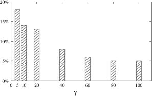
Figure 4: The picture shows — as a function of $\gamma=5,10,20,40,60,80,100$ s^-1 — the fraction of all trajectories (which have suffered a localization) that have been delocalized within the time interval $[t_{r},2\pi]$ seconds.

We have considered all trajectories which have been localized within the time interval $[0,2\pi]$ seconds, and we have counted the number of them which have gone through a delocalization within the time interval $[t_{r},2\pi]$, where $t_{r}$ is the reduction time for each single trajectory. As expected, for increasing values of $\gamma$, the fraction of all trajectories which are delocalized before time $t=2\pi$ seconds, decreases: once the state vector gets localized to any of the two eigenstates of $\sigma_{z}$, it fluctuates around it for a time interval which is longer, the greater the value of $\gamma$.

VI Transition from the “microscopic” to the “macroscopic” regime

We conclude the analysis of Eq. (1) by giving a general picture of how the evolution of $|\psi_{t}\rangle$ changes when moving from the “microscopic” ($\gamma\ll\omega$) regime to the “macroscopic” ($\gamma\gg\omega$) one.

Figure 5: The figures show two typical trajectories followed by the state vector in the Bloch sphere, for $\gamma=0.05$ s^-1 (Fig. a) and $\gamma=5$ s^-1 (Fig. b). In the first case, the Hamiltonian $H$ rotates the state vector along the $x$ axis of the Bloch sphere, while the reducing terms slowly move the rotation plane towards the $|+\rangle$ and $|-\rangle$ eigenstates. In the second case, the effect of the reduction terms is so strong that the state vector is rapidly driven towards the $|+\rangle$ eigenstate and then fluctuates around it, until it jumps to the other eigenstate $|-\rangle$. The arrows mark the starting point of the trajectories.

When $\gamma$ is vanishing small, the state vector simply rotates along the $x$–axis of the Bloch sphere, guided by the standard Hamiltonian $H=\hbar\omega\sigma_{x}$. As $\gamma$ increases — still remaining smaller than $\omega$ — $|\psi_{t}\rangle$ keeps rotating along the $x$–axis, but the stochastic terms shift the rotation plane towards the two eigenstates of $\sigma_{z}$ (see fig. (5a)).

When $\gamma$ becomes significantly greater than $\omega$, the state vector does not rotate any more around the $x$–axis of the Bloch sphere: it gets rapidly reduced to one of the two eigenstate of $\sigma_{z}$ (see fig. (5b)); moreover, if $\gamma$ is sufficiently large, the reductions occur with the correct quantum probabilities.

The state vector then fluctuates around the eigenstate to which it has been reduced for a time interval that — statistically — is longer, the greater the values of $\gamma$; accordingly, when $\omega$ can be neglected, the system behaves like a macroscopic system, regarding the physical properties of the spin along the $z$-axis: they always have a well–definite value.

VII Comparison with space–collapse models

Collapse models have been proposed in order to solve the measurement problem of quantum mechanics, and in particular to provide an explanation to the fact that macroscopic objects always have a definite position in space: accordingly, in most proposals on spontaneous collapse the localization operators are functions of the position operators. In this section, we confront the dynamics described by Eq. (1) with the properties of the collapse model proposed in ref. gpr . The stochastic Schrödinger equation of this model takes the form:

$$d|\psi_{t}\rangle = \left[-\frac{i}{\hbar}Hdt+\sqrt{\gamma}\int d^{3}x\left(N({\bf x})-\langle N_{t}({\bf x})\rangle\right)dW_{t}({\bf x})\right.$$ (12)

$$\left.-\frac{\gamma}{2}\int d^{3}x\left(N({\bf x})-\langle N_{t}({\bf x})\rangle\right)^{2}dt\,\right]|\psi_{t}\rangle,$$

where $\langle N_{t}({\bf x})\rangle=\langle\psi_{t}|N({\bf x})|\psi_{t}\rangle$ and $H$ is the standard Hamiltonian for the system under study. The “average density number operator” $N({\bf x})$ is defined as follows:

$$N({\bf x})=\left(\frac{\alpha}{2\pi}\right)^{3/2}\sum_{s}\int d^{3}y\,e^{\displaystyle-\frac{\alpha}{2}({\bf x}-{\bf y})^{2}}a^{\dagger}({\bf y},s)\,a({\bf y},s),$$ (13)

$a^{\dagger}({\bf y},s)$ and $a({\bf y},s)$ being, respectively, the creation and annihilation operators of a particle at point ${\bf y}$ with spin $s$; $W_{t}({\bf x})$ is a family of independent Wiener processes: ${\mathbb{E}}[dW_{t}({\bf x})]=0$, ${\mathbb{E}}[dW_{t}({\bf x})\,dW_{t}({\bf y})]=\delta^{(3)}({\bf x}-{\bf y})\,dt$.

Finally, the two parameters, $\alpha$ and $\gamma$, appearing in the model, have been taken equal to:

$$\frac{1}{\sqrt{\alpha}}\,=\,10^{-5}\,\makebox{cm},\quad\gamma\,=\,\lambda\left(\frac{4\pi}{\alpha}\right)^{\frac{3}{2}},\quad\lambda\,=\,10^{-17}\;\makebox{s${}^{-1}$}.$$ (14)

Eq. (12) has the same structure of Eq. (1) and, in all interesting physical situations, the Hamiltonian $H$ does not commute with the localization operators $a^{\dagger}({\bf y},s)\,a({\bf y},s)$: as a consequence the dynamics described by Eq. (12) is, qualitatively, analogous to that described by Eq. (1). We comment on the implications of our analysis of the spin–model (1), for the space–localization model given by Eq. (12).

Reduction mechanism. In the case of a free object, the analog of the time $\omega^{-1}$ can be reasonably identified with the time $T$ it takes for the spread $\Delta x$ of the center of mass of the object to change appreciably, e.g. to double its initial value; in the case of a free particle of mass $m$ (in one dimension), we have:

$$\Delta x(t)\;=\;\Delta x(t_{0})\,\sqrt{1+\frac{h^{2}[\Delta x(t_{0})]^{-4}}{4m^{2}}\,t^{2}},$$ (15)

so that $\Delta x(t)=2\Delta x(t_{0})$ when $t=T$, with:

$$T=\frac{\sqrt{12}m[\Delta x(t_{0})]^{2}}{h}.$$ (16)

In the above formula, we shall take $\Delta x(t_{0})=10^{-5}$ cm, which is the typical localization length of the model (compare with eq. (14)).

According to the numerical values given to the parameters $\alpha$ and $\gamma$, in the microscopic situation (when only one or a few constituents are present) we are in the situation where the characteristic time $T$ associated to the Hamiltonian is exceedingly smaller than the characteristic time $\lambda^{-1}$ associated to the reduction mechanism; for a particle like a proton, we have, e.g.:

$$T\;\sim\;10^{-7}\,\makebox{s}\quad\ll\quad\lambda^{-1}\;\simeq\;10^{17}\,\makebox{s}.$$ (17)

In this situation, the standard quantum dynamics of microscopic systems in not appreciably altered by the presence of the stochastic terms.

On the other hand, in the macroscopic case, as already mentioned, an “amplification mechanism” occurs: it can be shown gpr that the frequency $\Lambda$ associated to the reduction of the center of mass of a rigid body is approximately given by the formula: $\Lambda=N\lambda$, where $N$ is the number of constituents of the object. For an object of mass equal to 1 gr ($N\sim N_{\makebox{\tiny Avogadro}}$), we have:

$$T\;\sim\;10^{17}\,\makebox{s}\quad\gg\quad\Lambda^{-1}\;\sim\;10^{-7}\,\makebox{s}.$$ (18)

Accordingly, the characteristic time $T$ associated to a macroscopic object is many order of magnitudes greater than $\Lambda^{-1}$. In this situation, it can be proved that:

a) The reduction time is extremely well defined and small ($\sim 10^{-6}$ s), much smaller than the perception time of a human being. All macroscopic objects are localized in a very fast way, and superpositions of different macroscopic states cannot persist.

b) After the reduction as occurred, the wavefunction of the system is very well localized in space: for typical macroscopic objects its spread in position is $\sim 10^{-11}$ cm.

Of course, the wavefunction cannot have a compact support, since the Hamiltonian (when it does not commute with the position operators) would immediately turn it into a wavefunction with “tails” going off to infinity; anyway, the fraction of total wavefunction corresponding to the tails is of the order of $e^{-10^{18}}$, which means that they can be neglected for all practical purposes.

Probabilities. The reduction probabilities are almost exactly equal to the quantum probabilities and the outcomes of measurement processes follow the Born rule. Of course, the physical predictions of Eq. (12) are in principle different from those of standard quantum mechanics: this opens the way to the possibility of testing collapse models, especially at the mesoscopic level where the time scales of the quantum dynamics and the time scales of the reduction mechanism become comparable. Anyway, such kind of tests are difficult to implement as it is difficult to control all sources of noise which mask the effects of spontaneous localizations.

Delocalization process. We have seen in section IV that, when the spin–wavefunction has been localized into one of the two eigenstates of $\sigma_{z}$, it will sooner or later be driven by the dynamics of Eq. (1) into the other eigenstate and back. The dynamics of Eq. (12) displays a similar behavior.

After a macroscopic object has been localized in space (take its velocity equal to zero), there is a non zero probability that it gets delocalized and, shortly after that, localized again in a different region of space. Anyway, the probability that such an event occurs is exceedingly small (practically equal to zero), being proportional to the fraction of the wavefunction corresponding to its tails. Accordingly, when a macroscopic object gets localized, it stays localized practically forever.

Note also that this feature of space collapse is common to standard quantum mechanics as well: any macroscopic object, being described by a wavefunction with noncompact support, has a (vanishing small) probability of going through a quantum jump from a space region to a far away one.

Appendix I: Complete solutions of the equation for the statistical operator

The solutions of equations (3) are given as follows:

Over–damped case: $\gamma>2\omega$.

$$x(t) = a\,e^{-\gamma(1+\mu)t}\;+\;b\,e^{-\gamma(1-\mu)t}\;+\;1/2$$

$$y(t) = y_{0}\,e^{-2\gamma t}$$

$$z(t) = c\,e^{-\gamma(1-\mu)t}\;+\;d\,e^{-\gamma(1+\mu)t},$$ (19)

with:

$$a = -\frac{2\omega^{2}}{\gamma^{2}\mu(1+\mu)}\,x_{0}\;+\;\frac{\omega}{\gamma\mu}\,z_{0}\;+\;\frac{\omega^{2}}{\gamma^{2}\mu(1+\mu)}$$

$$b = \frac{2\omega^{2}}{\gamma^{2}\mu(1-\mu)}\,x_{0}\;-\;\frac{\omega}{\gamma\mu}\,z_{0}\;-\;\frac{\omega^{2}}{\gamma^{2}\mu(1-\mu)}$$

$$c = -\frac{\omega}{\gamma\mu}\,x_{0}\;+\;\frac{1+\mu}{2\mu}\,z_{0}\;+\;\frac{\omega}{2\gamma\mu}$$

$$d = \frac{\omega}{\gamma\mu}\,x_{0}\;-\;\frac{1-\mu}{2\mu}\,z_{0}\;-\;\frac{\omega}{2\gamma\mu}$$

$$\mu = \sqrt{1-\left(\frac{2\omega}{\gamma}\right)^{2}}$$ (20)

Critically damped case: $\gamma=2\omega$.

$$x(t) = [a\,+\,b\,t]\,e^{\displaystyle-\gamma\,t}\;+\;1/2$$

$$y(t) = y_{0}\,e^{\displaystyle-2\gamma t}$$

$$z(t) = [c\,+\,d\,t]\,e^{\displaystyle-\gamma\,t},$$ (21)

with:

$$a = x_{0}-\frac{1}{2}$$

$$b = (2x_{0}-1)\omega\,-\,\gamma z_{0}$$

$$c = z_{0}$$

$$d = (2x_{0}-1)\omega\,-\,\gamma z_{0}.$$ (22)

Under–damped case: $\gamma<2\omega$.

$$x(t) = \left[a\cos(\lambda t)\,+\,b\sin(\lambda t)\right]e^{\displaystyle-\gamma t}\;+\;1/2$$

$$y(t) = y_{0}\,e^{\displaystyle-2\gamma t}$$

$$z(t) = \left[c\cos(\lambda t)\,+\,d\sin(\lambda t)\right]e^{\displaystyle-\gamma t},$$ (23)

with:

$$a = x_{0}-\frac{1}{2}$$

$$b = \frac{\gamma}{\lambda}\,x_{0}\,-\,\frac{2\omega}{\lambda}\,z_{0}-\frac{\gamma}{2\lambda}$$

$$c = z_{0}$$

$$d = \frac{1}{\lambda}\left(2\omega x_{0}\,-\,\omega\,-\,\gamma\,z_{0}\right)$$

$$\lambda = \gamma\,\sqrt{\left(\frac{2\omega}{\gamma}\right)^{2}-1}$$ (24)

Appendix II: A note on the numerical simulation

To solve eq. (1), we have used the simple Euler algorithm, which proved to be satisfactory for the purposes of the article. To test the goodness of the simulation, we have compared the analytical evolution of ${\mathbb{E}}\,[|\langle+|\psi_{t}\rangle|^{2}]=\langle+|\rho(t)|+\rangle$ with the average value of $|\langle+|\psi_{t}\rangle|^{2}$ over many sample trajectories, obtained by solving eq. (1) numerically (see Fig. 6).

Figure 6: The two dotted curves represent the (analytical) evolution $\langle+|\rho(t)|+\rangle$, with $\gamma=100$ s^-1 (upper curve) and $\gamma=5$ s^-1 (lower curve). The continuous curves show the average value of $|\langle+|\psi_{t}\rangle|^{2}$ over 100000 trajectories of $|\psi_{t}\rangle$, for the same values of $\gamma$. For the values of the time step, see the text.

While analyzing the data, we have seen that for large values of $\gamma$ — i.e. when the reduction mechanism becomes extremely rapid — the numerical simulation was not as good as expected. For such a reason we have decided to decrease the time step during the first $0.1$ s, obtaining a sensible improvement.

We have made different tests on the choice of the time steps and number of trials and, taking also into account the time required by our CPU for elaborating the data, we have found that the best choice (according to the previously mentioned criterion) was to take:

Time step for $t\leq 0.1$ s:	$10^{-7}$
Time step for $t>0.1$ s:	$10^{-3}$
Number of trials:	100000.

References

- (1) E.B. Davies, “Quantum theory of open systems” (Academic Press, London, 1976).
- (2) D. Giulini, E. Joos, C. Kiefer, J. Kupsch, I.–O. Stamatescu and H.D. Zeh, Decoherence and the Appearance of a Classical World in Quantum Theory (Springer, Berlin, 1996).
- (3) M.B. Plenio and P.L. Knight, Rev. Mod. Phys. 70, 101 (1998).
- (4) B. Vacchini, Phys. Rev. Lett. 84, 1374 (2000). Phys. Rev. E 63, 66115 (2001).
- (5) H.P. Breuer and F. Petruccione, “The theory of open quantum systems” (Oxford University Press, Oxford, 2002).
- (6) G. C. Ghirardi, P. Pearle and A. Rimini, Phys. Rev. A 42, 78 (1990). G.C. Ghirardi, R. Grassi and P. Pearle, Found. Phys. 20, 1271 (1990). G.C. Ghirardi, R. Grassi and A. Rimini, Phys. Rev. A 42, 1057 (1990). G.C. Ghirardi, R. Grassi and F. Benatti, Found. Phys. 25, 5 (1995).
- (7) G.C. Ghirardi, Phys. Lett. A 262, 1 (1999).
- (8) P. Pearle, Phys. Rev. D 13, 857 (1976). Phys. Rev. Lett. 53, 1775 (1984). Phys. Rev. A 39, 2277 (1989).
- (9) L. Diósi, Phys. Lett. A 132, 233 (1988). J. Phys. A 21, 2885 (1988). Phys. Rev. A 40, 1165 (1989). Phys. Rev. A 42, 5086 (1990).
- (10) V.P. Belavkin, in Lecture Notes in Control and Information Science, edited by A. Blaquière (Springer, Berlin, 1988), Vol. 121, p. 245; V.P. Belavkin and P. Staszewski, Phys. Lett. A 140, 355 (1989). Phys. Rev. A 45, 1347 (1992).
- (11) A. Barchielli, Quantum Opt. 2, 423 (1990). Int. J. Theor. Phys. 32, 2221 (1993).
- (12) Ph. Blanchard and A. Jadczyk, Phys. Lett. A 175, 157 (1993). Ann. der Physik 4, 583 (1995). Phys. Lett. A 203, 260 (1995).
- (13) N. Gisin and J. Percival, Phys. Lett. A 167, 315 (1992). J. Phys. A 26, 2233 (1993); 26, 2243 (1993). N. Gisin and I. Percival, Journ. Phys. A 25, 5677 (1992). N. Gisin and M. Rigo, Journ. Phys. A 28, 7375 (1995).
- (14) I. Percival, Quantum State Diffusion (Cambridge University Press, Cambridge, 1998).
- (15) L.P. Hughston, Proc. R. Soc. London A 452, 953 (1996).
- (16) S.L. Adler and L.P. Horwitz: Journ. Math. Phys. 41, 2485 (2000). S.L. Adler and T.A. Brun: Journ. Phys. A 34, 4797 (2001). S.L. Adler, D.C. Brody, T.A. Brun and L.P. Hughston, Journ. Phys. A 34, 8795 (2001). S.L. Adler, Journ. Phys. A 35, 841 (2002).
- (17) A. Bassi and G.C. Ghirardi: Phys. Rept. 379, 257 (2003).
- (18) G. Lindblad, Commun. Math. Phys. 48, 119 (1976).
- (19) H. Spohn, Rev. Mod. Phys. 53, 569 (1980).
- (20) L. Arnold, “Stochastic Differential Equations: Theory and Applications” (Wiley, New York, 1971).
- (21) P.E. Kloeden and E. Platen, “Numeical Solutions of Stochastic Differential Equations” (Springer–Verlag, Berlin, 1992).