]http://www.quantware.ups-tlse.fr

Quantum computation of the Anderson transition in presence of imperfections

Abstract

We propose a quantum algorithm for simulation of the Anderson transition in disordered lattices and study numerically its sensitivity to static imperfections in a quantum computer. In the vicinity of the critical point the algorithm gives a quadratic speedup in computation of diffusion rate and localization length, comparing to the known classical algorithms. We show that the Anderson transition can be detected on quantum computers with $7-10$ qubits.

The problem of metal-insulator transition of noninteracting electrons in a disordered potential was pioneered by Anderson in 1958 anderson58 . Since then it continues to attract an active interest of researchers all over the world (see e.g. lee85 ; kramer ; mirlin and Refs. therein). In addition to analytical and experimental studies of the problem an important contribution to the understanding of its properties was made with the help of numerical simulations based on various computational methods adapted to the physics of this phenomenon. Indeed, the numerical studies allowed to obtain some values of critical exponents in the vicinity of the transition and to study certain system characteristics at the critical point including level spacing statistics and conductance fluctuations for the cases of different symmetries and system dimensions (see e.g. kramer ; mirlin ; shklovski ; zharekeshev ; slevin99 ). These numerical simulations are performed with the help of modern supercomputers and are at the border of their computational capacity.

The recent progress in quantum computation demonstrated that due to quantum parallelism certain tasks can be performed much faster on a quantum computer (see chuang and Refs. therein). The most known example is the Shor algorithm for factorization of large integers shor which is exponentially faster than any known classical algorithm. A number of efficient quantum algorithms was also proposed for simulation of quantum evolution of certain Hamiltonians including many-body quantum systems lloyd ; ortiz and problems of quantum chaos schack ; georgeot ; benenti . In Ref. georgeot it was shown that the evolution propagator in a regime of dynamical or Anderson localization can be simulated efficiently on a quantum computer. However, the algorithm proposed there requires a significant number of redundant qubits and is not accessible for an experimental implementation with a first generation of quantum computers composed of 5 - 10 qubits.

In this paper we propose a quantum algorithm for a quantum dynamics in the regime of Anderson localization. This algorithm requires no redundant qubits thus using the available $n_{q}$ qubits in an optimal way. The propagation on a unit time step is performed in $O(n_{q}^{2})$ quantum elementary gates while any known classical algorithm requires $O(2^{n_{q}})$ operations for a vector of size $N=2^{n_{q}}$. Due to these properties the Anderson transition can be already detected on a quantum computer with 7 - 10 qubits. The basic elements of the algorithm involve one qubit rotations, controlled phase shift $C(\phi)$, controlled-NOT gate $C_{N}$ and the Quantum Fourier Transform (QFT) chuang . All these quantum operations have been already realized for 3 - 7 qubits in the NMR-based quantum computations reported in Refs. cory ; chuang1 . Thus the main obstacle for experimental detection of the Anderson transition in quantum computations is related to the effects of external decoherence paz and residual static imperfections georgeot1 which restrict the number of available quantum gates. The results obtained for operating quantum algorithms benenti ; terraneo show that the effects of static imperfections affect the accuracy of quantum computation in a stronger way comparing to the case of random noisy gate errors. Due to that in this paper we concentrate our studies on the case of static imperfections investigating their impact on the system properties in the vicinity of the Anderson transition.

To study the effects of static imperfections in quantum computations of the Anderson transition we choose the generalized kicked rotator model described by the unitary evolution of the wave function $\psi$:

$$\begin{array}[]{c}\bar{\psi}={\hat{U}}\psi=\exp(-iV(\theta,t))\exp(-iH_{0}({\hat{n}}))\psi\;\;.\end{array}$$ (1)

Here $\bar{\psi}$ is the new value of $\psi$ after one map iteration given by the unitary operator ${\hat{U}}$, $H_{0}(n)$ gives the rotational phases in the basis of momentum ${\hat{n}}=-i\partial/\partial\theta$, the kick potential $V(\theta,t)$ depends on the rotator phase $\theta$ and time $t$ measured in number of kicks, $\psi(\theta+2\pi)=\psi(\theta)$. For $V(\theta,t)=k\cos\theta$ and $H_{0}=Tn^{2}/2$ one has the kicked rotator model described in detail in izrailev . The evolution given by (1) results from the Hamiltonian $H=H_{0}(n)+V(\theta,t)\delta_{1}(t)$, where $\delta_{1}(t)$ is a periodic $\delta$-function with period 1 and $(n,\theta)$ are conjugated variables. In the case when the potential $V(\theta,t)=-2\tan^{-1}(2k(\cos\theta+\cos{\omega_{1}t}+\cos{\omega_{1}t}))$ depends quasi-periodically on time $t$ the model can be exactly reduced to the three-dimensional (3D) Lloyd model 3f . Indeed, the time dependence of $V(\theta,t)$ can be eliminated by introduction of extended phase-space with a replacement $H_{0}\rightarrow H_{0}(n)+\omega_{1}n_{1}+\omega_{2}n_{2}$. Then the linear dependence on quantum numbers $n_{1,2}$ gives fixed frequency rotations of the conjugated phases $\theta_{1,2}=\omega_{1,2}t$. The extensive studies performed in 3f showed that this model displays the Anderson metal-insulator transition at $k=k_{c}\approx 0.5$ with the critical exponents being close to the values found in other 3D solid state models. In this paper following borgonovi we choose in (1) the potential $V(\theta,t)=k(1+0.75\cos\omega_{1}t\cos\omega_{2}t)\cos\theta$ with $\omega_{1}=2\pi\lambda^{-1}$, $\omega_{2}=2\pi\lambda^{-2}$ and $\lambda=1.3247...$ being the real root of the cubic equation $x^{3}-x-1=0$. The rotation phases $H_{0}(n)$ are randomly distributed in the interval $(0,2\pi)$. This model shows the Anderson transition at $k_{c}\approx 1.8$ borgonovi with the characteristics similar to those of the Lloyd model studied in 3f .

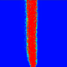
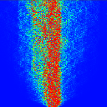
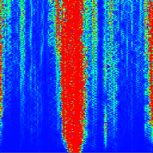
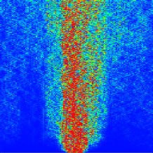
Figure 1: (color online) The time evolution of the probability distribution $|\psi_{n}|^{2}$ in the localized (left column, $k=1.2$) and delocalized (right column, $k=2.4$) phases for $n_{q}=7$ qubits ($N=2^{n_{q}}$), with $0\leq t\leq 400$ (vertical axis) and $-N/2<n\leq N/2$ (horizontal axis); $k_{c}=1.8$. The color is proportional to probability: blue/black for zero and red/white for maximal values. The strength of static imperfections is $\epsilon=\mu=0$ for top row and $\epsilon=\mu=10^{-4}$ for bottom row.

The quantum algorithm simulating the time evolution of this model is constructed in the following way. The quantum states $n=0,...,N-1$ are represented by one quantum register with $n_{q}$ qubits so that $N=2^{n_{q}}$. The initial state with all probability at $n_{0}=0$ corresponds to the state $|00...0>$ (momentum $n$ changes on a circle with $N$ levels). The phase rotation $U_{T}=\exp(-iH_{0}(n))$ in the momentum basis $n$ is performed with the help of quantum random phase generator built from two unitary operators $U^{(1)}_{T}$ and $U^{(2)}_{T}$. The operator $U^{(1)}_{T}=\prod_{j=1}^{n_{q}}e^{i\phi_{j}\sigma^{z}_{j}}$ gives rotation of qubit $j$ by a random phase $\phi_{j}$. Here and below $\sigma^{x},\sigma^{y},\sigma^{z}$ are Pauli matrices. To improve the independence of quantum phases we then apply the operator $U^{(2)}_{T}=\prod_{k=1}^{M}C_{N}(i_{M-k},j_{M-k})\prod_{k=1}^{M}e^{i\phi_{j_{k}}^{\prime}\sigma^{z}_{j_{k}}}C_{N}(i_{k},j_{k})$. This transformation represents a random sequence with $M$ one-qubit phase shifts $e^{i\phi_{j_{k}}^{\prime}\sigma^{z}_{j_{k}}}$ and controlled-NOT gates $C_{N}(i_{k},j_{k})$ followed by the inversed sequence of controlled-NOT gates $C_{N}(i_{M-k},j_{M-k})$. Here $C_{N}(i_{k},j_{k})$ inverts the qubit $j_{k}$ if the qubit $i_{k}$ is 1; $i_{k},j_{k}$ and phases $\phi_{j_{k}}^{\prime}$ are chosen randomly. The resulting random quantum phase generator $U_{T}=U_{T}^{(2)}U_{T}^{(1)}$ gives more and more independent random phases with the increase of $M$. We use $M\approx 2n_{q}$ (at $n_{q}\approx 10$) that according to our tests generates good random phase values. This step involves $3M+n_{q}$ quantum gates. After that the kick operator $U_{k}=\exp(-ik(t)\cos\theta)$ is performed as follows. First, with the help of the QFT the wave function is transformed from momentum $n$ to phase $\theta$ representation in $O(n_{q}^{2}/2)$ gates. Then $\theta$ can be written in the binary representation as $\theta/2\pi=0.a_{1}a_{2}..a_{n_{q}}$ with $a_{i}=0$ or 1. It’s convenient to use the notation $\theta=\pi a_{1}+\bar{\theta}$ to single out the most significant qubit. Then due to the relation $\cos\theta=(-1)^{a_{1}}\cos\bar{\theta}=\sigma^{z}_{1}\cos\bar{\theta}$ the kick operator takes the form $U_{k}=e^{-ik(t)\cos\theta}=e^{-i\sigma^{z}_{1}k(t)\cos\bar{\theta}}$, where $\sigma^{(z,x)}_{1}$ act on the first qubit. This operator can be approximated to an arbitrary precision by a sequence of one-qubit gates applied to the first qubit and the diagonal operators $S^{m}=e^{ima_{1}\bar{\theta}}$. The $S-$operators are given by the product of $n_{q}-1$ two-qubit gates as $S^{m}=\prod_{j=2}^{n_{q}}C_{1,j}(\pi m2^{-j+1})$ where controlled phase shift gate $C_{j_{1},j_{2}}(\phi)$ makes a phase shift $e^{i\phi}$ if both qubits $j_{1,2}$ are 1. Then we introduce the unitary operator $R_{\gamma}(\bar{\theta})=HS^{1}H\;e^{-i\frac{\gamma}{2}\sigma^{z}_{1}}\;HS^{-2}H\;e^{-i\frac{\gamma}{2}\sigma^{z}_{1}}\;HS^{1}H$ where $H=(\sigma^{z}_{1}+\sigma^{x}_{1})/\sqrt{2}$ is the Hadamard gate. It can be exactly reduced to the form $R_{\gamma}(\bar{\theta})=\cos^{2}\frac{\gamma}{2}-\sin^{2}\frac{\gamma}{2}\cos(2\bar{\theta})-i\sigma^{z}_{1}\sin\gamma\cos(\bar{\theta})+i\sigma^{x}_{1}\sin^{2}\frac{\gamma}{2}\sin(2\bar{\theta})$ and hence for small $\gamma$ we have $R_{\gamma}(\bar{\theta})=e^{-i\sigma^{z}_{1}\gamma\cos\bar{\theta}}+i\sigma^{x}_{1}\frac{\gamma^{2}}{4}\sin(2\bar{\theta})+O(\gamma^{3})$. The term with $\gamma^{2}$ can be eliminated using the symmetric representation $R_{\gamma/2}(\bar{\theta})R_{\gamma/2}(-\bar{\theta})=HS^{1}H\;e^{-i\frac{\gamma}{4}\sigma^{z}_{1}}\;HS^{-2}H\;e^{-i\frac{\gamma}{2}\sigma^{z}_{1}}\;HS^{2}H\;e^{-i\frac{\gamma}{4}\sigma^{z}_{1}}\;HS^{-1}H=e^{-i\sigma^{z}_{1}\gamma\cos(\bar{\theta})}+O(\gamma^{3})$. Thus the kick operator is given by $U_{k}=(R_{\gamma/2}(\bar{\theta})R_{\gamma/2}(-\bar{\theta}))^{l}+O(l\gamma^{3})$ where the number of steps $l=k/\gamma$ and we used in our numerical simulations the small parameter $\gamma=k/l\approx 0.2$ that gives $l\approx 5-10$ for $k\sim 1-2$. After that the state is transfered to the momentum representation by the QFT. Thus an iteration (1) is performed for $2^{n_{q}}$ states in $n_{g}$ elementary gates where $n_{g}=2[k/\gamma](n_{q}+2)+n_{q}^{2}+6n_{q}+3M+9$ with the square brackets denoting the integer part. This algorithm is optimal for the kicked rotator model with moderate values of $k$ where $n_{g}$ value remains reasonable. It can be easily generalized to $d$ dimensions.

In our numerical simulations we study the effects of static quantum computer imperfections considered in georgeot1 ; benenti ; terraneo . In this case all gates are perfect but between gates $\psi$ accumulates a phase factor $e^{i{\hat{\varphi}}}$ with ${\hat{\varphi}}=\sum_{j}(\eta_{j}\sigma^{z}_{j}+\mu_{j}\sigma^{x}_{j}\sigma^{x}_{j+1})$. Here $\eta_{j},\mu_{j}$ vary randomly with $j=1,...,n_{q}$, $\eta_{j}$ represents static one-qubit energy shifts, $-\epsilon/2\leq\eta_{j}\leq\epsilon/2$, and $\mu_{j}$ represents static inter-qubit couplings on a circular chain, $-\mu/2\leq\mu_{j}\leq\mu/2$.

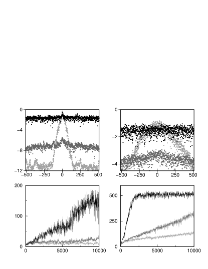
Figure 2: Top row: logarithm of probability $\log_{10}|\psi_{n}|^{2}$ vs. momentum $n$ after $t=10000$ iterations; dark gray curves are shifted down by 5 (left) and 2 (right). Bottom row: dependence of IPR $\xi$ on time $t$. The left/right column corresponds to localized/delocalized phase at $k=1.2$ and $k=2.4$ respectively. The three curves represent $\epsilon=0;2\times 10^{-5};6\times 10^{-5}$ with color changing from light gray to black with increase of $\epsilon$; $\mu=\epsilon$, $n_{q}=10$.

An example of time evolution of probability distribution in the momentum representation $n$ is shown in Fig. 1. Below the Anderson transition ($k<k_{c}$) the probability remains bounded near initial value $n_{0}$, while above it ($k>k_{c}$) a diffusive spreading in $n$ takes place. Comparing to the ideal quantum computation the static imperfections lead to probability transfer on levels located far away from the center of the wave packet. This effect is related to the structure of the QFT where a mismatch in the quantum gates generates high harmonics. As a result static imperfections create a plateau in the probability distribution which level grows with the increase of $\epsilon$ and $\mu$ (see Fig. 2). This leads to an artificial diffusion of the second moment of the distribution $<n^{2}>=<\psi_{n}|(n-n_{0})^{2}|\psi_{n}>$. Since the plateau in probability extends over all $N$ levels the rate of this diffusion grows exponentially with $n_{q}$ at fixed $\epsilon,\mu$ (data not shown). A similar effect was discussed in song for the quantum computation of the kicked rotator with noisy gates. Due to that the most appropriate characteristic to study is the Inverse Participation Ratio (IPR) $\xi$ which is extensively used in systems with localization kramer ; mirlin and which determines the number of levels on which the wave function is concentrated $(\sum_{n}|\psi_{n}|^{4}=1/\xi)$. In contrast to $<n^{2}>$, the IPR $\xi$ remains stable with respect to noise in the gates during polynomially large times song .

Figure 3: Dependence of the IPR $\xi$ and the excitation probability $W$ (full and dashed curves for left and right scales respectively) on the kick strength $k$ for $n_{q}=10$ and $t\geq 10^{5}$, $\epsilon=0;10^{-5};2\times 10^{-5};4\times 10^{-5};8\times 10^{-5}$ (corresponding to curves from right to left); $\mu=0$.

The variation of $\xi$ with time and $\epsilon,\mu$ is shown in Fig. 2. For moderate imperfections, during a rather long time interval $\xi$ remains close to its value in the exact algorithm. However, at very large times $t\geq 10^{5}$ it saturates at some value which depends on $k$ and $\epsilon,\mu$. A typical example of such a dependence is presented in Fig. 3. Here, $\xi$ shows a sharp jump from small ($\xi\sim 1$) to large ($\xi\sim N$) values which takes place in a narrow interval of $k$ values. This is a manifestation of the Anderson transition from localized to delocalized states. The critical point $k_{c}$ can be numerically defined as a such value of $k$ at which $\xi$ is at the middle between its two limiting values. The data of Fig. 3 show that the critical point $k_{c}(\epsilon)$ decreases with the increase of the strength of imperfections. The physical origin of this effect is related to the additional transitions induced by static imperfections which naturally lead to a delocalization at a lower value of $k$ compared to the ideal computation. Another method to detect the position of the critical point $k_{c}(\epsilon)$ in presence of imperfections is to measure the two most significant qubits which code the value of momentum $n$. After a few tens of measurements of first 2 qubits one determines the probability $W=\sum_{n=(N/4,3N/4)}|\psi_{n}|^{2}$. At sufficiently large $t$ this probability shows a sharp jump from a value $W=0$ to $W\approx 0.5$ when $k$ is varied. This allows to determine the critical point and gives the values of $k_{c}(\epsilon)$ close to those obtained via IPR $\xi$ (see Fig. 3).

Figure 4: Dependence of the shift of the critical point $\Delta k_{c}(\epsilon)=k_{c}-k_{c}(\epsilon)$ on rescaled imperfection strength $\tilde{\epsilon}=\epsilon n_{g}\sqrt{n_{q}}$ for $\epsilon=2\times 10^{-5}$ (diamonds), $4\times 10^{-5}$ (triangles) and $8\times 10^{-5}$ (squares); open/full symbols are for $\mu=0$, $8\leq n_{q}\leq 13$ and $\mu=\epsilon$, $8\leq n_{q}\leq 11$ respectively; $k_{c}=1.8$. The dashed lines show the scaling relation (2).

The shift of the critical point $\Delta k_{c}(\epsilon)=k_{c}-k_{c}(\epsilon)$ depends on $\epsilon,\mu$ and $n_{q}$. From the IPR data obtained for various $\epsilon,\mu,n_{q}$, see Fig. 4, we find that the global parameter dependence can be described by the scaling relation

$$\Delta k_{c}(\epsilon)=A\tilde{\epsilon}^{\;\alpha},\;\;{\tilde{\epsilon}}=\epsilon n_{g}\sqrt{n_{q}}$$ (2)

The data fit gives $A=3.0$, $\alpha=0.64$ for $\mu=0$ and $A=4.8$, $\alpha=0.68$ for $\mu=\epsilon$. This result can be understood from the following arguments. According to benenti ; terraneo the time scale $t_{f}$, on which the fidelity of quantum computation is close to unity, is determined by the parameter $\tilde{\epsilon}$ ($t_{f}\sim 1/\tilde{\epsilon}$). Thus, an effective matrix element induced by static imperfections between ideal localized eigenstates can be estimated as $U_{ef}\sim\tilde{\epsilon}Q\sim\tilde{\epsilon}/l^{\beta}$, where $Q$ is a typical overlap of localized eigenstates which for the Anderson localization in $d$ dimensions can be estimated as $Q\sim l^{-\beta}$ with $\beta=d/2$ and $l$ being the localization length for the exact algorithm (see a discussion in benenti1 for $d=1$). The imperfections induced delocalization should take place when $U_{ef}$ exceeds the level spacing in a block of size $l$ ($U_{ef}>\Delta_{l}\sim 1/l^{d}$). Taking into account that near the critical point the localization length scales as $l\sim\Delta k^{-\nu}$ with $\nu\sim 1.5$ (see kramer ; 3f ; borgonovi ) we obtain that $\alpha=1/(\nu(d-\beta))=2/\nu d$. The obtained value of $\alpha$ would give a reasonable value of $\nu\approx 1.0$ but in our model (1) the situation is more complicated. Indeed, the dynamics in (1) takes place in one dimension and hence one expects $\beta=1/2$ and $\nu\approx 0.6$. The later value has a noticeable difference from a usually expected value kramer ; 3f ; borgonovi . A possible reason for this discrepancy can be related to the fact that in the algorithm the perturbations give far away transitions (see Fig. 1) which effectively decrease the value of $\beta$, also near the critical point the correlations in the matrix elements can play an important role. Further studies are required to clarify this point.

Finally, let us note that in the vicinity of critical point the number of states grows with time as $n^{d}\sim t$ kramer ; mirlin ; slevin99 . Hence, the number of classical operations for $t$ kicks can be estimated as $n_{gcl}\sim tN^{d}\log^{d}N\sim t^{2}\log^{d}t$ while the quantum algorithm will need $n_{g}\sim dn_{q}^{2}t\sim t\log^{2}t$ gates assuming $d$ quantum registers with $N^{d}=2^{dn_{q}}\sim t$ states. The coarse-grained characteristics of the probability distribution can be determined from few measurements of most significant qubits, e.g. $W$ as in Fig.3. Thus, even if each step in (1) is efficient, the speedup is only quadratic near the critical point. Above the critical point we have diffusive growth with $n^{d}\sim t^{d/2}$ and the speedup is stronger: $n_{gcl}\sim n_{g}^{(1+d/2)}$ for $d>2$.

This work was supported in part by the NSA and ARDA under ARO contract No. DAAD19-01-1-0553 and the EC IST-FET project EDIQIP. We thank CalMiP at Toulouse and IDRIS at Orsay for access to their supercomputers.

References

• (1) P.W.ย Anderson, Phys. Rev. 109, 1492 (1958).
• (2) P.A.ย Lee and T.V.ย Ramakrishnan, Rev. Mod. Phys. 57, 287 (1985).
• (3) B.ย Kramer and A.ย MacKinnon, Rep. Prog. Phys. 56, 1469 (1993).
• (4) A.D.ย Mirlin, Phys. Rep. 326, 259 (2000).
• (5) B.I.ย Shklovskii, B.ย Shapiro, B.R.ย Sears, P.ย Lambrianides and H.B.ย Shore, Phys. Rev. B 47, 11487 (1993).
• (6) I.K.ย Zharekeshev and B.ย Kramer, Ann. Phys. (Leipzig) 7, 442 (1998).
• (7) T.ย Ohtsuki, K.Slevin and T.ย Kawarabayashi, Ann. Phys. (Leipzig) 8, 655 (1999); Y.ย Asada, K.ย Slevin, and T.ย Ohtsuki, Phys. Rev. Lett. 89, 256601 (2002).
• (8) M.A.ย Nielsen and I.L.ย Chuang Quantum Computation and Quantum Information, Cambridge Univ. Press, Cambridge (2000).
• (9) P.W.Shor, in Proc. 35th Annual Symposium on Foundation of Computer Science, Ed. S.Goldwasser (IEEE Computer Society, Los Alamitos, CA, 1994), p.124
• (10) S.ย Lloyd, Science 273, 1073 (1996).
• (11) G.ย Ortiz, J.E.ย Gubernatis, E.ย Knill, and R.Laflamme, Phys. Rev. A 64, 22319 (2001).
• (12) R.ย Schack, Phys. Rev. A 57, 1634 (1998).
• (13) B.ย Georgeot, and D.L.ย Shepelyansky, Phys. Rev. Lett. 86, 2890 (2001).
• (14) G.ย Benenti, G.ย Casati, S.ย Montangero, and D.L.ย Shepelyansky, Phys. Rev. Lett. 87, 227901 (2001).
• (15) Y.S.ย Weinstein, S.ย Lloyd, J.ย Emerson, and D.G.ย Cory, Phys. Rev. Lett. 89, 157902 (2002).
• (16) L.M.K.Vandersypen, M. Steffen, G. Breyta, C.S. Yannoni, M.H. Sherwood, and I.L. Chuang, Nature 414, 883 (2001).
• (17) C.Miguel, J.P.Paz and W.H.Zurek, Phys. Rev. Lett. 78, 3971 (1997).
• (18) B.Georgeot and D.L.Shepelyansky, Phys. Rev. E 62, 3504 (2000); 62, 6366 (2000).
• (19) M.Terraneo and D.L.Shepelyansky, Phys. Rev. Lett. 90, 257902 (2003).
• (20) F.M.Izrailev, Phys. Rep. 196, 299 (1990).
• (21) G.Casati, I.Guarneri and D.L.Shepelyansky, Phys. Rev. Lett. 62, 345 (1989); F.Borgonovi and D.L.Shepelyansky, Physica D 109, 24 (1997).
• (22) F.Borgonovi and D.L.Shepelyansky, J. de Physique I France 6, 287 (1996).
• (23) P.H.Song and D.L.Shepelyansky, Phys. Rev. Lett. 86, 2162 (2001).
• (24) G.ย Benenti, G.ย Casati, S.ย Montangero, and D.L.ย Shepelyansky, Phys. Rev. A 67, 052312 (2003).