IN WIGNER-LIKE EQUATIONS

VIA MULTIRESOLUTION

Antonina N. Fedorova, Michael G. Zeitlin

IPME RAS, St. Petersburg, V.O. Bolshoj pr., 61, 199178, Russia

e-mail: zeitlin@math.ipme.ru

e-mail: anton@math.ipme.ru

http://www.ipme.ru/zeitlin.html

http://www.ipme.nw.ru/zeitlin.html Pattern Formation in Wigner-like Equations via Multiresolution A. N. Fedorova and M. G. Zeitlin IPME RAS, St. Petersburg, V.O. Bolshoj pr., 61, 199178, Russia E-mail: zeitlin@math.ipme.ru, anton@math.ipme.ru Abstract We present the application of the variational-wavelet analysis to the quasiclassical calculations of the solutions of Wigner/von Neumann/Moyal and related equations corresponding to the nonlinear (polynomial) dynamical problems. (Naive) deformation quantization, the multiresolution representations and the variational approach are the key points. We construct the solutions via the multiscale expansions in the generalized coherent states or high-localized nonlinear eigenmodes in the base of the compactly supported wavelets and the wavelet packets. We demonstrate the appearance of (stable) localized patterns (waveletons) and consider entanglement and decoherence as possible applications. Abstract We present the application of the variational-wavelet analysis to the quasiclassical calculations of the solutions of Wigner/von Neumann/Moyal and related equations corresponding to the nonlinear (polynomial) dynamical problems. (Naive) deformation quantization, the multiresolution representations and the variational approach are the key points. We construct the solutions via the multiscale expansions in the generalized coherent states or high-localized nonlinear eigenmodes in the base of the compactly supported wavelets and the wavelet packets. We demonstrate the appearance of (stable) localized patterns (waveletons) and consider entanglement and decoherence as possible applications. Presented at Joint 28th ICFA Advanced Beam Dynamics

& Advanced & Novel Accelerators Workshop on

QUANTUM ASPECTS OF BEAM PHYSICS

and Other Critical Issues of Beams in Physics and Astrophysics

January 7-11, 2003, Hiroshima University, Higashi-Hiroshima, Japan

1 Wigner-like Equations

In this paper we consider the applications of a numerical-analytical technique based on local nonlinear harmonic analysis (wavelet analysis, generalized coherent states analysis) to the quasiclassical calculations in nonlinear (polynomial) dynamical problems in the Wigner-Moyal approach. The corresponding class of Hamiltonians has the form

$$\hat{H}(\hat{p},\hat{q})=\frac{\hat{p}^{2}}{2m}+U(\hat{p},\hat{q}),$$ (1)

where $U(\hat{p},\hat{q})$ is an arbitrary polynomial function on $\hat{p}$, $\hat{q}$, and plays the key role in many areas of physics [1], [2]. The particular cases, related to some physics models, are considered in [3]-[12]. Our goals are some attempt of classification and the explicit numerical-analytical constructions of the existing quantum states in the class of models under consideration. There is a hope on the understanding of relation between the structure of initial Hamiltonians and the possible types of quantum states and the qualitative type of their behaviour. Inside the full spectrum there are at least three possibilities which are the most important from our point of view: localized states, chaotic-like or/and entangled patterns, localized (stable) patterns (definitions can be found below). All such states are interesting in the different areas of physics (e.g., [1], [2]) discussed below. Our starting point is the general point of view of a deformation quantization approach at least on the naive Moyal/Weyl/Wigner level [1], [2]. The main point of such approach is based on ideas from [1], which allow to consider the algebras of quantum observables as the deformations of commutative algebras of classical observables (functions). So, if we have as a model for classical dynamics the classical counterpart of Hamiltonian (1) and the Poisson manifold $M$ (or symplectic manifold or Lie coalgebra, etc) as the corresponding phase space, then for quantum calculations we need first of all to find an associative (but non-commutative) star product $*$ on the space of formal power series in $\hbar$ with coefficients in the space of smooth functions on $M$ such that

$$f*g=fg+\hbar\{f,g\}+\sum_{n\geq 2}\hbar^{n}B_{n}(f,g),$$ (2)

where $\{f,g\}$ is the Poisson brackets, $B_{n}$ are bidifferential operators. Kontsevich gave the solution to this deformation problem in terms of the formal power series via the sum over graphs and proved that for every Poisson manifold M there is a canonically defined gauge equivalence class of star-products on M. Also there are the nonperturbative corrections to power series representation for $*$ [1]. In the naive calculations we may use the simple formal rule:

$$* \equiv \exp\Big{(}\frac{i\hbar}{2}(\overleftarrow{\partial}_{q}\overrightarrow{\partial}_{p}-\overleftarrow{\partial}_{p}\overrightarrow{\partial}_{q})\Big{)}$$ (3)

In this paper we consider the calculations of the Wigner functions $W(p,q,t)$ (WF) corresponding to the classical polynomial Hamiltonian $H(p,q,t)$ as the solution of the Wigner-von Neumann equation [2]:

$$i\hbar\frac{\partial}{\partial t}W=H*W-W*H$$ (4)

and related Wigner-like equations. According to the Weyl transform, a quantum state (wave function or density operator $\rho$) corresponds to the Wigner function, which is the analogue in some sense of classical phase-space distribution [2]. We consider the following form of differential equations for time-dependent WF, $W=W(p,q,t)$:

$$W_{t}=\frac{2}{\hbar}\sin\Big{[}\frac{\hbar}{2}(\partial^{H}_{q}\partial^{W}_{p}-\partial^{H}_{p}\partial^{W}_{q})\Big{]}\cdot HW$$ (5)

which is a result of the Weyl transform of von Neumann equation

$$i\hbar\frac{\partial\rho}{\partial t}=[H,\rho]$$ (6)

In our case (1) we have the following decomposition [2] ($U=U(q)$ in the following only for simplicity, but the case $U=U(p,q)$ can be considered analogously):

$$\frac{\partial W}{\partial t}=T+U,$$ (7)

where

$$U=\sum_{i=0}^{\infty}\frac{(i\hbar/2)^{2l}}{(2l+1)!}\frac{d^{2l+1}U(q)}{dq^{2l+1}}\frac{\partial^{2l+1}}{\partial p^{2l+1}}W(p,q;t)$$ (8)

$$T=-\frac{p}{m}\frac{\partial}{\partial q}W(p,q;t)$$ (9)

Let $\{|E\rangle,E\}$ be the full set of discrete/continuous eigenfunctions (eigenvalues)

$$H|E\rangle=E|E\rangle$$ (10)

then we have the following representation for the Moyal function:

$$W_{E^{\prime\prime},E^{\prime}}(q,p)\equiv\frac{1}{2\pi\hbar}\int^{\infty}_{-\infty}d\xi e^{-ip\xi/h}(q+\frac{1}{2}\xi|E^{\prime\prime}\rangle\langle E^{\prime}|q-\frac{1}{2}\xi\rangle$$ (11)

which is reduced to the standard WF in the case $E^{\prime}=E^{\prime\prime}$: $W_{E,E}(p,q)\equiv W(p,q)$. As a result, the time independent Moyal function generates the time evolution of the WF. The corresponding integral representation contains the initial value of the density operator $\rho(0)$ as a factor [2]. The Moyal function satisfies the following system of (pseudo)differential equations

$$\Big{[}\frac{p^{2}}{2m}+U-\frac{\hbar^{2}}{8m}\frac{\partial^{2}}{\partial q^{2}}+\sum^{\infty}_{i=1}\frac{(-1)^{l}(\hbar/2)^{2l}}{(2l)!}\frac{d^{2l}U}{dq^{2l}}\frac{\partial^{2l}}{\partial p^{2l}}\Big{]}W_{E^{\prime\prime},E^{\prime}}$$

$$=\frac{E^{\prime}+E^{\prime\prime}}{2}W_{E^{\prime\prime},E^{\prime}}$$ (12)

$$\Big{[}\frac{p}{m}\frac{\partial}{\partial q}-\frac{dU}{dq}\frac{\partial}{\partial p}-\sum^{\infty}_{i=1}\frac{(-1)^{l}(\hbar/2)^{2l}}{(2l+1)!}\frac{d^{2l+1}U}{dq^{2l+1}}\frac{\partial^{2l+1}}{\partial p^{2l+1}}\Big{]}W_{E^{\prime\prime},E^{\prime}}$$

$$=\frac{i}{\hbar}(E^{\prime\prime}-E^{\prime})W_{E^{\prime\prime},E^{\prime}}$$ (13)

really nonlocal/pseudodifferential for arbitrary Hamiltonians. But in case of polynomial Hamiltonians (1) we have only a finite number of terms in the corresponding series. Also, in the stationary case after Weyl-Wigner mapping we have the following equation on WF in c-numbers [2]:

$$\Big{(}\frac{p^{2}}{2m}+\frac{\hbar}{2i}\frac{p}{m}\frac{\partial}{\partial q}-\frac{\hbar^{2}}{8m}\frac{\partial^{2}}{\partial q^{2}}\Big{)}W(p,q)+$$ (14)

$$U\Big{(}q-\frac{\hbar}{2i}\frac{\partial}{\partial p}\Big{)}W(p,q)=\epsilon W(p,q)$$

After expanding the potential $U$ into the Taylor series we have two real partial differential equations which correspond to the mentioned before particular case of the Moyal equations (12), (13).

Our approach, presented below, in some sense is motivated by the analysis of the following standard simple model considered in [2]. Let us consider model of interaction of nonresonant atom with quantized electromagnetic field:

$$\hat{H}=\frac{\hat{p}_{x}^{2}}{2m}+U(\hat{x}),\qquad U(\hat{x})=U_{0}(z,t)g(\hat{x})\hat{a}^{+}\hat{a}$$ (15)

where potential $U$ depends on creation/annihilation operators and some polynomial on $\hat{x}$ operator function (or approximation) $g(\hat{x})$. It is possible to solve Schroedinger equation

$$i\hbar\frac{\mathrm{d}|\Psi>}{\mathrm{d}t}=\hat{H}|\Psi>$$ (16)

by the simple ansatz

$$|\Psi(t)>=\sum_{-\infty}^{\infty}w_{n}\int\mathrm{d}x|\Psi_{n}(x,t)|x>\otimes|n>$$ (17)

which leads to the hierarchy of analogous equations with potentials created by n-particle Fock subspaces

$$i\hbar\frac{\partial\Psi_{n}(x,t)}{\partial t}=\Big{\{}\frac{\hat{p}_{x}^{2}}{2m}+U_{0}(t)g(x)n\Big{\}}\Psi_{n}(x,t)$$ (18)

where $\Psi_{n}(x,t)$ is the probability amplitude of finding the atom at the time $t$ at the position $x$ and the field in the $n$ Fock state. Instead of this, we may apply the Wigner approach starting with proper full density matrix

$$\hat{\rho}=|\Psi(t)><\Psi(t)|=$$ (19)

$$\sum_{n^{\prime},n^{\prime\prime}}w_{n^{\prime}}w^{*}_{n^{\prime\prime}}\int\mathrm{d}x^{\prime}\int\mathrm{d}x^{\prime\prime}\Psi_{n^{\prime}}(x^{\prime},t)\Psi^{*}_{n^{\prime\prime}}(x^{\prime\prime},t)|x^{\prime}><x^{\prime\prime}|\otimes|n^{\prime}><n^{\prime\prime}|$$

Standard reduction gives pure atomic density matrix

$$\hat{\rho}_{a}\equiv\int^{\infty}_{n=0}<n|\hat{\rho}|n>=$$ (20)

$$\sum|w_{n}|^{2}\int\mathrm{d}x^{\prime}\int\mathrm{d}x^{\prime\prime}\Psi_{n}(x^{\prime},t)\Psi^{*}_{n}(x^{\prime\prime},t)|x^{\prime}><x^{\prime\prime}|$$

Then we have incoherent superposition

$$W(x,p,t)=\sum^{\infty}_{n=0}|w_{n}|^{2}W_{n}(x,p,t)$$ (21)

of the atomic Wigner functions

$$W_{n}(x,p,t)\equiv\frac{1}{2\pi\hbar}\int\mathrm{d}\xi{\rm exp}\Big{(}-\frac{i}{\hbar}p\xi\Big{)}\Psi^{*}_{n}(x-\frac{1}{2}\xi,t)\Psi_{n}(x+\frac{1}{2}\xi,t)$$ (22)

corresponding to the atom motion in the potential $U_{n}(x)$ (which is not more than polynomial in $x$) generated by $n$-level Fock state. They are solutions of proper Wigner equations:

$$\frac{\partial W_{n}}{\partial t}=-\frac{p}{m}\frac{\partial W_{n}}{\partial x}+\sum^{\infty}_{\ell=0}\frac{(-1)^{\ell}(\hbar/2)^{2\ell}}{(2\ell+1)!}\frac{\partial^{2\ell+1}U_{n}(x)}{\partial x^{2\ell+1}}\frac{\partial^{2\ell+1}W_{n}}{\partial p^{2\ell+1}}$$ (23)

In the following section we’ll generalize this construction and we are interested in description of entanglement in the Wigner formalism.

The next example describes the decoherence process. Let we have collective and environment subsystem with their own Hilbert spaces

$$\mathcal{H}=\mathcal{H}_{c}\otimes\mathcal{H}_{e}$$ (24)

Relevant dynamics are described by three parts including interaction

$$H=H_{c}\otimes I_{e}+I_{c}\otimes H_{e}+H_{int}$$ (25)

For analysis, we can choose Lindblad master equation [2]

$$\dot{\rho}=\frac{1}{i\hbar}[H,\rho]-\sum_{n}\gamma_{n}(L^{+}_{n}L_{n}\rho+\rho L^{+}_{n}L_{n}-2L_{n}\rho L^{+}_{n})$$ (26)

which preserves the positivity of density matrix and it is Markovian but it is not general form of exact master equation. Other choice is Wigner transform of master equation [2] and it is more preferable for us

$$\dot{W}=\{H,W\}_{PB}+$$ (27)

$$\sum_{n\geq 1}\frac{\hbar^{2n}(-1)^{n}}{2^{2n}(2n+1)!}\partial^{2n+1}_{x}U(x)\partial_{p}^{2n+1}W(x,p)+2\gamma\partial_{p}pW+D\partial^{2}_{p}W$$

In the next section we consider the variation-wavelet approach for the solution of all these Wigner-like equations (6)-(9), (12), (14), (23), (26), (27) for the case of an arbitrary polynomial $U(q,p)$, which corresponds to a finite number of terms in the series from (8), (12), (13), (14), (23), (27) or to proper finite order of $\hbar$. Our approach is based on the extension of our variational-wavelet approach [3]-[12]. Wavelet analysis is some set of mathematical methods, which gives the possibility to work with well-localized bases in functional spaces and gives maximum sparse forms for the general type of operators (differential, integral, pseudodifferential) in such bases. These bases are the natural generalization of standard coherent, squeezed, thermal squeezed states [2], which correspond to quadratical systems (pure linear dynamics) with Gaussian Wigner functions. Because the affine group of translations and dilations (or more general group, which acts on the space of solutions) is inside the approach (in wavelet case), this method resembles the action of a microscope. We have a contribution to the final result from each scale of resolution from the whole underlying infinite scale of spaces. Our main goals are an attempt of classification and construction of possible nontrivial states in the system under consideration. We are interested in the following states: localized, entangled patterns, localized (stable) patterns. We start from the corresponding definitions (at this stage these definitions have only qualitative character).

1. By localized state (localized mode) we mean the corresponding (particular) solution of the system under consideration which is localized in maximally small region of the phase space.

2. By chaotic/entangled pattern we mean some solution (or asymptotics of solution) of the system under consideration which has equidistribution of energy spectrum in a full domain of definition.

3. By localized pattern (waveleton) we mean (asymptotically) stable solution localized in relatively small region of the whole phase space (or a domain of definition). In this case all energy is distributed during some time (sufficiently large) between few localized modes (from point 1) only.

Numerical calculations explicitly demonstrate the quantum interference of generalized coherent states, pattern formation from localized eigenmodes and the appearance of (stable) localized patterns (waveletons).

2 Variational Multiscale Representation

We obtain our multiscale/multiresolution representations for solutions of Wigner-like equations via a variational-wavelet approach. We represent the solutions as decomposition into modes related to the hidden underlying set of scales [13]:

$$W(t,q,p)=\displaystyle\bigoplus^{\infty}_{i=i_{c}}\delta^{i}W(t,q,p)$$ (28)

where value $i_{c}$ corresponds to the coarsest level of resolution $c$ or to the internal scale with the number $c$ in the full multiresolution decomposition of underlying functional space ($L^{2}$, e.g.) corresponding to problem under consideration:

$$V_{c}\subset V_{c+1}\subset V_{c+2}\subset\dots$$ (29)

and $p=(p_{1},p_{2},...),q=(q_{1},q_{2},...),x_{i}=(p_{1},q_{1},....,p_{i},q_{i})$ are coordinates in phase space. In the following we may consider as fixed as variable numbers of particles. The second case corresponds to quantum statistical ensemble (via “wignerization” procedure) and will be considered in details elsewhere [12].

We introduce the Fock-like space structure

$$H=\sum^{\infty}_{n=0}\bigoplus H^{n}$$ (30)

for the set of n-particle wave functions (states):

$$W=\{W_{0},W_{1}(x_{1};t),W_{2}(x_{1},x_{2};t),\dots,W_{N}(x_{1},\dots,x_{N};t),\dots\},$$ (31)

where $W_{p}(x_{1},\dots,x_{p};t)\in H^{p}$, $H^{0}=C,\quad H^{p}=L^{2}(R^{6p})$ (or any different proper functional space), $W\in$ $H^{\infty}=H^{0}\oplus H^{1}\oplus\dots\oplus H^{p}\oplus\dots$ with the natural Fock space like norm (guaranteeing the positivity of the full measure):

$$(W,W)=W^{2}_{0}+\sum_{i}\int W^{2}_{i}(x_{1},\dots,x_{i};t)\prod^{i}_{\ell=1}\mu_{\ell}.$$ (32)

First of all we consider $W=W(t)$ as a function of time only, $W\in L^{2}(R)$, via multiresolution decomposition which naturally and efficiently introduces the infinite sequence of the underlying hidden scales [13]. We have the contribution to the final result from each scale of resolution from the whole infinite scale of spaces. We consider a multiresolution decomposition of $L^{2}(R)$ (of course, we may consider any different and proper for some particular case functional space) which is a sequence of increasing closed subspaces $V_{j}\in L^{2}(R)$ (subspaces for modes with fixed dilation value):

$$...V_{-2}\subset V_{-1}\subset V_{0}\subset V_{1}\subset V_{2}\subset...$$ (33)

The closed subspace $V_{j}(j\in{\bf Z})$ corresponds to the level $j$ of resolution, or to the scale j and satisfies the following properties: let $W_{j}$ be the orthonormal complement of $V_{j}$ with respect to $V_{j+1}$: $V_{j+1}=V_{j}\bigoplus W_{j}.$ Then we have the following decomposition:

$$\{W(t)\}=\bigoplus_{-\infty<j<\infty}W_{j}\qquad{\rm or}\qquad\{W(t)\}=\overline{V_{0}\displaystyle\bigoplus^{\infty}_{j=0}W_{j}},$$ (34)

in case when $V_{0}$ is the coarsest scale of resolution. The subgroup of translations generates a basis for the fixed scale number: ${\rm span}_{k\in Z}\{2^{j/2}\Psi(2^{j}t-k)\}=W_{j}.$ The whole basis is generated by action of the full affine group:

$${\rm span}_{k\in Z,j\in Z}\{2^{j/2}\Psi(2^{j}t-k)\}={\rm span}_{k,j\in Z}\{\Psi_{j,k}\}=\{W(t)\}.$$ (35)

Let the sequence $\{V_{j}^{t}\},V_{j}^{t}\subset L^{2}(R)$ correspond to multiresolution analysis on the time axis, $\{V_{j}^{x_{i}}\}$ correspond to multiresolution analysis for coordinate $x_{i}$, then $V_{j}^{n+1}=V^{x_{1}}_{j}\otimes\dots\otimes V^{x_{n}}_{j}\otimes V^{t}_{j}$ corresponds to the multiresolution analysis for the $n$-particle function $W_{n}(x_{1},\dots,x_{n};t)$. E.g., for $n=2$:$\qquad V^{2}_{0}=\{f:f(x_{1},x_{2})=$ $\sum_{k_{1},k_{2}}a_{k_{1},k_{2}}\phi^{2}(x_{1}-k_{1},x_{2}-k_{2}),\ a_{k_{1},k_{2}}\in\ell^{2}(Z^{2})\},$ where $\phi^{2}(x_{1},x_{2})=\phi^{1}(x_{1})\phi^{2}(x_{2})=\phi^{1}\otimes\phi^{2}(x_{1},x_{2}),$ and $\phi^{i}(x_{i})\equiv\phi(x_{i})$ form a multiresolution basis corresponding to $\{V_{j}^{x_{i}}\}$. If $\{\phi^{1}(x_{1}-\ell)\},\ \ell\in Z$ form an orthonormal set, then $\phi^{2}(x_{1}-k_{1},x_{2}-k_{2})$ form an orthonormal basis for $V^{2}_{0}$. So, the action of the affine group generates multiresolution representation of $L^{2}(R^{2})$. After introducing the detail spaces $W^{2}_{j}$, we have, e.g. $V^{2}_{1}=V^{2}_{0}\oplus W^{2}_{0}.$ Then the 3-component basis for $W^{2}_{0}$ is generated by the translations of three functions

$$\Psi^{2}_{1}=\phi^{1}(x_{1})\otimes\Psi^{2}(x_{2}),\ \Psi^{2}_{2}=\Psi^{1}(x_{1})\otimes\phi^{2}(x_{2}),\ \Psi^{2}_{3}=\Psi^{1}(x_{1})\otimes\Psi^{2}(x_{2}).$$

Also, we may use the rectangle lattice of scales and one-dimensional wavelet decomposition: f(x_1,x_2)=∑_i,ℓ;j,k⟨f,Ψ_i,ℓ⊗Ψ_j,k⟩Ψ_j,ℓ⊗Ψ_j,k(x_1,x_2), where the basis functions $\Psi_{i,\ell}\otimes\Psi_{j,k}$ depend on two scales $2^{-i}$ and $2^{-j}$. After constructing the multidimensional basis we may apply one of the variational procedures from [3]-[12]. We obtain our multiscale/multiresolution representations (formulae (40) below) via the variational wavelet approach for the following formal representation of the systems from the Section 1 (or its approximations).

Let $L$ be an arbitrary (non)linear differential/integral operator with matrix dimension $d$ (finite or infinite), which acts on some set of functions from $L^{2}(\Omega^{\otimes^{n}})$: $\quad\Psi\equiv\Psi(t,x_{1},x_{2},\dots)=\Big{(}\Psi^{1}(t,x_{1},x_{2},\dots),\dots$, $\Psi^{d}(t,x_{1},x_{2},\dots)\Big{)}$, $\quad x_{i}\in\Omega\subset{\bf R}^{6}$, $n$ is the number of particles:

$$L\Psi\equiv L(Q,t,x_{i})\Psi(t,x_{i})=0,$$ (36)

where

$$Q\equiv Q_{d_{0},d_{1},d_{2},\dots}(t,x_{1},x_{2},\dots,\partial/\partial t,\partial/\partial x_{1},\partial/\partial x_{2},\dots,\int\mu_{k})=$$

$$\sum_{i_{0},i_{1},i_{2},\dots=1}^{d_{0},d_{1},d_{2},\dots}q_{i_{0}i_{1}i_{2}\dots}(t,x_{1},x_{2},\dots)\Big{(}\frac{\partial}{\partial t}\Big{)}^{i_{0}}\Big{(}\frac{\partial}{\partial x_{1}}\Big{)}^{i_{1}}\Big{(}\frac{\partial}{\partial x_{2}}\Big{)}^{i_{2}}\dots\int\mu_{k}.$$ (37)

Let us consider now the $N$ mode approximation for the solution as the following ansatz:

$$\Psi^{N}(t,x_{1},x_{2},\dots)=\sum^{N}_{i_{0},i_{1},i_{2},\dots=1}a_{i_{0}i_{1}i_{2}\dots}A_{i_{0}}\otimes B_{i_{1}}\otimes C_{i_{2}}\dots(t,x_{1},x_{2},\dots).$$ (38)

We shall determine the expansion coefficients from the following conditions (different related variational approaches are considered in [3]-[12]:

$$\ell^{N}_{k_{0},k_{1},k_{2},\dots}\equiv\int(L\Psi^{N})A_{k_{0}}(t)B_{k_{1}}(x_{1})C_{k_{2}}(x_{2})\mathrm{d}t\mathrm{d}x_{1}\mathrm{d}x_{2}\dots=0.$$ (39)

Thus, we have exactly $dN^{n}$ algebraical equations for $dN^{n}$ unknowns $a_{i_{0},i_{1},\dots}$. This variational approach reduces the initial problem to the problem of solution of functional equations at the first stage and some algebraical problems at the second. We consider the multiresolution expansion as the second main part of our construction. So, the solution is parametrized by the solutions of two sets of reduced algebraical problems, one is linear or nonlinear (depending on the structure of the operator $L$) and the rest are linear problems related to the computation of the coefficients of the algebraic equations (39). These coefficients can be found by some wavelet methods by using the compactly supported wavelet basis functions for the expansions (38). As a result the solution of the equations from Section 1 has the following multiscale or multiresolution decomposition via nonlinear high-localized eigenmodes

$$W(t,x_{1},x_{2},\dots)=\sum_{(i,j)\in Z^{2}}a_{ij}U^{i}\otimes V^{j}(t,x_{1},x_{2},\dots),$$

$$V^{j}(t)=V_{N}^{j,slow}(t)+\sum_{l\geq N}V^{j}_{l}(\omega_{l}t),\quad\omega_{l}\sim 2^{l},$$ (40)

$$U^{i}(x_{s})=U_{M}^{i,slow}(x_{s})+\sum_{m\geq M}U^{i}_{m}(k^{s}_{m}x_{s}),\quad k^{s}_{m}\sim 2^{m},$$

which corresponds to the full multiresolution expansion in all underlying time/space scales. The formulae (40) give the expansion into a slow part and fast oscillating parts for arbitrary $N,M$. So, we may move from the coarse scales of resolution to the finest ones for obtaining more detailed information about the dynamical process. In this way one obtains contributions to the full solution from each scale of resolution or each time/space scale or from each nonlinear eigenmode. It should be noted that such representations give the best possible localization properties in the corresponding (phase)space/time coordinates. Formulae (40) do not use perturbation techniques or linearization procedures. Numerical calculations are based on compactly supported wavelets and related wavelet families [13] and on evaluation of the accuracy on the level $N$ of the corresponding cut-off of the full system regarding norm (32):

$$\|W^{N+1}-W^{N}\|\leq\varepsilon.$$ (41)

So, by using wavelet bases with their best (phase) space/time localization properties we can describe localized (coherent) structures in quantum systems with complicated behaviour. The modeling demonstrates the appearance of different (stable) pattern formation from high-localized coherent structures or chaotic behaviour. Our (nonlinear) eigenmodes are more realistic for the modelling of nonlinear classical/quantum dynamical process than the corresponding linear gaussian-like coherent states. Here we mention only the best convergence properties of the expansions based on wavelet packets, which realize the minimal Shannon entropy property and the exponential control of convergence of expansions like (40) based on the norm (32). Fig. 1 shows the high-localized eigenmode contribution to the WF, while Fig. 2, 3 give the representations for the full solutions, constructed from the first 6 eigenmodes (6 levels in formula (40)), and demonstrate the stable localized pattern formation (waveleton) and complex chaotic-like behaviour. Fig. 3 corresponds to (possible) result of superselection (einselection) [2] after decoherence process started from Fig. 2 or Fig. 4. Fig. 5 and Fig. 6 demonstrate time steps during appearance of entangled states. It should be noted that we can control the type of behaviour on the level of the reduced algebraical system (39) [12].

Acknowledgements

We are very grateful to Prof. Pisin Chen (SLAC) for invaluable encouragement, support and patience.

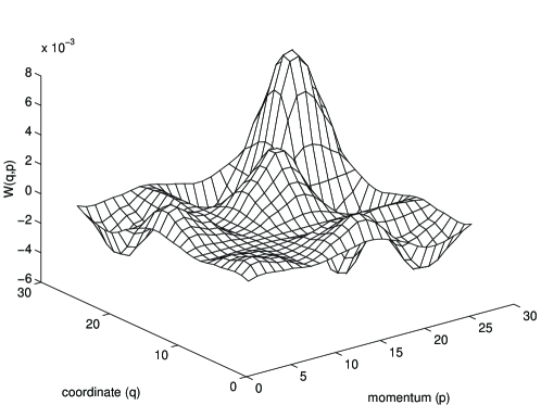
Figure 1: Localized mode contribution to Wigner function.

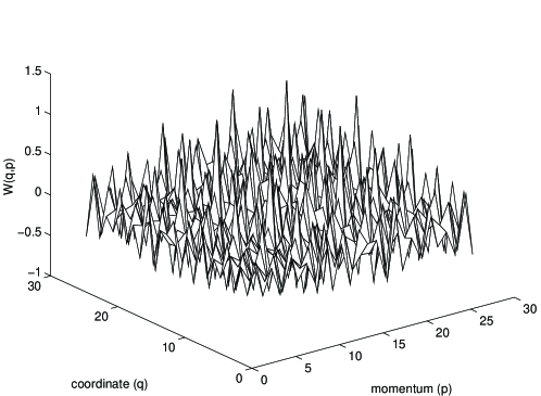
Figure 2: Chaotic-like Wigner function.

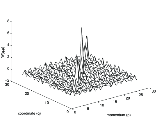
Figure 3: Localized pattern-like (waveleton) Wigner function.

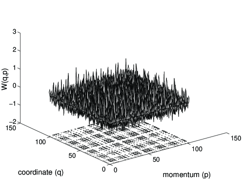
Figure 4: Entangled-like Wigner function.

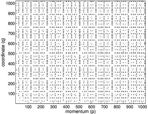
Figure 5: Section of the coarse level approximation for Wigner function.

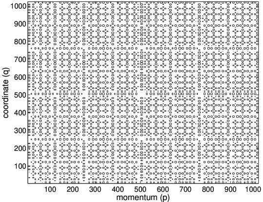
Figure 6: Section of the finest level approximation for Wigner function.

References

- [1] D. Sternheimer, Los Alamos preprint, math.QA/9809056, T. Curtright, T. Uematsu, C. Zachos, Los Alamos preprint: hep-th/0011137.
- [2] W. P. Schleich, Quantum Optics in Phase Space, Wiley, 2000, W. Zurek, Los Alamos preprint: quant-ph/0105127.
- [3] A.N. Fedorova, M.G. Zeitlin, Math. and Comp. in Simulation, 46, 527, 1998.
- [4] A.N. Fedorova, M.G. Zeitlin, New Applications of Nonlinear and Chaotic Dynamics in Mechanics, Ed. F. Moon, 31, 101 Kluwer, 1998.
- [5] A.N. Fedorova, M.G. Zeitlin, CP405, 87, American Institute of Physics, 1997. Los Alamos preprint: physics/9710035.
- [6] A.N. Fedorova, M.G. Zeitlin and Z. Parsa, CP468, 48, 69, American Institute of Physics, 1999. Los Alamos preprints: physics/990262, 9902063.
- [7] A.N. Fedorova, M.G. Zeitlin, The Physics of High Brightness Beams, Ed. J. Rosenzweig, 235, World Scientific, 2001. Los Alamos preprint: physics/0003095.
- [8] A.N. Fedorova, M.G. Zeitlin, Quantum Aspects of Beam Physics, Ed. P. Chen, 527, 539, World Scientific, 2002; arXiv preprints: physics/0101006, 0101007.
- [9] A.N. Fedorova, M.G. Zeitlin, Proceedings EPAC2002, pp. 1323, 1344, 1434, 1482, 1595, EPS-IGA/CERN, 2002, arXiv preprints: physics/0206049, 0206050, 0206051, 0206052, 0206053.
- [10] A.N. Fedorova, M.G. Zeitlin, Proceedings in Applied Mathematics and Mechanics, Volume 1, Issue 1, 399, 432, Wiley-VCH, 2002, arXiv preprints: nlin.PS/0206024, physics/0206054.
- [11] A.N. Fedorova, M.G. Zeitlin, Nuclear Inst. and Methods in Physics Research, A, vol 502/2-3 657, 660, 2003, arXiv preprints: quant-ph/0212166, physics/0212115.
- [12] A.N. Fedorova, M.G. Zeitlin, Progress in Nonequilibrium Green’s Functions II, Ed. M. Bonitz and D. Semkat, World Scientific, 481, 2003, arXiv preprint: physics/0212066 and in press.
- [13] Y. Meyer, Wavelets and Operators, Cambridge Univ. Press, 1990.