Abstract

We have developed a fully quantized model for EIT in which the decay rates are taken into account. In this model, the general form of the susceptibility and group velocity of the probe laser we obtained are operators. Their expectation value and fluctuation can be obtained on the Fock space. Furthermore the uncertainty of the group velocity under very weak intensity of the controlling laser and the uncertainty relation between the phase operator of coupling laser and the group velocity are approximately given. Considering the decay rates of various levels, we may analyze the probe laser near resonance in detail and calculate the fluctuation in both absorption and dispersion. We also discuss how the fully quantized model reduces to a semiclassical model when the mean photon numbers of the coupling laser is getting large.
PACS numbers: 42.50.Gy, 42.65.-k, 42.65.An

1 Introduction

Controlling the phase coherence in ensembles of multilevel atoms has led to the observation of many striking phenomena in the propagation of near-resonant light. The notable examples include ultraslow light pulse propagation, light storage, lasing without inversion and EIT[1, 2, 3, 4, 5, 6]. Among these striking phenomena, ultraslow light speed and superluminality look more attracting. The drastic reductions in the group velocity of pulses were discussed in Ref.[5] and recent experiments have taken the reduction of the speed of light to extreme limits (shown in Refs.[6, 7] and even to zero[8, 9]. On the other way, the superluminal velocity was also observed in the abnormal-dispersion media[10]. In the most previous work the phenomenon of EIT and the accompanying enhancement of the index of refraction and susceptibility are treated using semiclassical theory in which both the coupling and probe lasers were treated as classical. In such a treatment, the occurrence of EIT requires the coupling laser to be much stronger than the probe laser. In Ref.[8], Fleischhauer and Lukin treated the probe laser as quantized, and showed that the quantum description of laser is more fundamental than the classical one, having advantages in uncovering new effects of EIT. In Ref.[11] Kuang et al. treated both the coupling and probe lasers as quantized and they pointed out that in general the group velocity depends on the intensity of the coupling as well as probe laser. But they ignored decay rates of various levels, so their treatment is essentially a time-independent approach. Obviously, if the decay rates are incorporated, it needs to solve the evolution equation of the density matrix, which is difficult in a fully quantized treatment.

Based on the results of the previous works, the strength of the coupling laser needs to be modified from finite to zero to decelerate and stop the input pulse[8, 9]. But when coupling laser is very weak, we can no longer treat the coupling laser as classical, in other words, we should develop a fully quantized model for EIT.

In this paper, both the coupling and probe lasers are treated as quantized. First we give a straightforward discussion of the case with no decay rates In section 2.1, and then take the decay rates into account in section 2.2. We shall obtain the general form of density matrix and susceptibility and analyze several cases in section 2.2: In part(a) we discuss how the fully quantized model reduces to the model given by Refs[8, 9] when the mean photon number of the coupling laser is large; Part(b) we obtain that the general form of susceptibility and group velocity is operators, the expectation value of which can be obtained by act the operators on the Fock space and there is fluctuation. We calculate the uncertainty of group velocity numerically and give an approximate uncertainty relation between the phase operator of coupling laser and the group velocity; Part(c) we discuss the more general case where both the probe and coupling lasers are weak and have similar intensities.

2 The theoretical model

2.1 The case with no decay rates

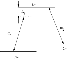
Figure 1: Energy levels of a $\Lambda$-type atom

Let us start from the well-known three-level $\Lambda$-type configuration atom (Fig.1) whose energy levels assumed to be $E_{a}>E_{c}>E_{b}$. They interact with two quantized fields, probe and coupling ones. The two low levels $|b\!\!>$ and $|c\!\!>$ are coupled to the upper one $|a\!\!>$ separately and initially the atom is in the ground state $|b\!\!>$. The frequency of the coupling laser $\omega_{2}=\omega_{ac}$ and the probe laser $\omega_{1}=\omega_{ab}-\Delta_{1}$, where $\Delta_{1}$ is the detuning of the probe laser. Here both the probe and coupling lasers are quantized. In the interaction picture the Hamiltonian of the system is[12]:

$$H^{I} = H_{0}^{I}+H_{1}^{I}$$ (1)

$$H_{0}^{I} = E_{a}|a\!\!><\!\!a|+E_{b}|b\!\!><\!\!b|+E_{c}|c\!\!><\!\!c|$$ (2)

$$-\hbar[\Delta_{1}(|a\!\!><\!\!a|+|c\!\!><\!\!c|)]+\omega_{1}\hat{a}_{1}^{\dagger}\hat{a}_{1}+\omega_{2}\hat{a}_{2}^{\dagger}\hat{a}_{2}$$

$$H_{1}^{I} = \hbar\Delta_{1}(|a\!\!><\!\!a|+|c\!\!><\!\!c|)-\hbar(g_{1}\hat{a}_{1}|a\!\!><\!\!b|+g_{2}\hat{a}_{2}|a\!\!><\!\!c|+\rm{H.C})$$ (3)

where $\hat{a}_{i}$ and $\hat{a}_{i}^{\dagger}$ ($i=1,2$) are the annihilation and creation operators of the probe (for $i=1$) and coupling (for $i=2$) laser modes respectively, and $g_{i}$ the coupling constants. Assuming the detuning $\Delta_{1}$ small, we shall find the solution for the dark-state $|\psi_{0}\!\!>$ of the system by perturbative approximation. The perturbation with the first order was given in Ref.[11]:

$$|\psi_{0}\!\!> = |\psi_{0}^{(0)}\!\!>+|\psi_{0}^{(1)}\!\!>$$ (4)

$$= \frac{\Omega_{2}}{\Omega}|b,n_{1},n_{2}\!\!>-\frac{2\Omega_{1}\Omega_{2}}{\Omega^{3}}\Delta_{1}|a,n_{1}-1,n_{2}\!\!>-\frac{\Omega_{1}}{\Omega}|c,n_{1}-1,n_{2}+1\!\!>$$

With the energy eigenvalue $\hbar\frac{\Omega_{1}^{2}}{\Omega^{2}}\Delta_{1}$, i.e., $H_{1}^{I}|\psi_{0}\!\!>=\hbar\frac{\Omega_{1}^{2}}{\Omega^{2}}\Delta_{1}|\psi_{0}\!\!>$. The second-ordered perturbation can be calculated:

$$|\psi_{0}\!\!> = |\psi_{0}^{0}\!\!>+|\psi_{0}^{1}\!\!>+|\psi_{0}^{2}\!\!>$$ (5)

$$= \left(\frac{\Omega_{2}}{\Omega}-\frac{4\Omega_{1}^{2}\Omega_{2}^{3}}{\Omega^{7}}\Delta_{1}^{2}\right)|b,n_{1},n_{2}\!\!>-\frac{2\Omega_{1}\Omega_{2}}{\Omega^{3}}\Delta_{1}|a,n_{1}-1,n_{2}\!\!>$$

$$-\left(\frac{\Omega_{1}}{\Omega}+\frac{4\Omega_{1}\Omega_{2}^{4}}{\Omega^{7}}\Delta_{1}^{2}\right)|c,n_{1}-1,n_{2}+1\!\!>$$

where $|n_{1},n_{2}\!\!>$ is the usual two-mode Fock basis. $\Omega_{1}=2g_{1}\sqrt{n_{1}}$ , $\Omega_{2}=2g_{2}\sqrt{n_{2}+1}$ and $\Omega=\sqrt{\Omega_{1}^{2}+\Omega_{2}^{2}}$. Suppose the coupling and probe lasers are in a two-mode coherent state $|\alpha,\beta\!\!>$ with$\alpha,\beta$ the real for simplicity[12] and the atom is initially in the ground state $|b\!\!>\!\!\otimes|\alpha,\beta\!\!>$. If we consider the ideal case in which the decay rates of various levels are ignored and initially $\Omega_{1}=0$ with $\Omega_{2}$ finite, then proceed to turn $\Omega_{2}$ down while slowly turning $\Omega_{1}$ on. During the course, the state $|\psi_{0}(t)\!\!>$ of the system will evolve adiabatically, so from (4) or (5) we can get the density matrix of the system. Further we can calculate the susceptibility of the system. If the mean photon number of the coupling laser $\bar{n}_{\alpha}=\alpha^{2}$ and the probe laser $\bar{n}_{\beta}=\beta^{2}$ are large, i.e., in semiclassical limit, from (5) we have

$$\rho_{ab}(\omega_{1})=-\frac{2\bar{\Omega}_{1}\bar{\Omega}_{2}^{2}}{(\bar{\Omega}_{1}^{2}+\bar{\Omega}_{2}^{2})^{2}}\Delta_{1}+\frac{8\bar{\Omega}_{1}^{3}\bar{\Omega}_{2}^{4}}{(\bar{\Omega}_{1}^{2}+\bar{\Omega}_{2}^{2})^{5}}\Delta_{1}^{3}$$ (6)

where $\bar{\Omega}_{i}=\bar{\Omega}_{i}(\bar{n}_{\alpha},\bar{n}_{\beta})\,(i=1,2)$ are the Rabi frequencies of the coupling and probe lasers, with $\wp_{ab}N\rho_{ab}(\omega_{1})=\epsilon_{0}\chi(\omega_{1})\hat{E}_{1}(\omega_{1})$, The susceptibility is given by:

$$\chi(\omega_{1})=-\frac{4N|\wp_{ab}|^{2}\bar{\Omega}_{2}^{2}}{\hbar\epsilon_{0}(\bar{\Omega}_{1}^{2}+\bar{\Omega}_{2}^{2})^{2}}\Delta_{1}+\frac{16|\wp_{ab}|^{2}N\bar{\Omega}_{1}^{2}\bar{\Omega}_{2}^{4}}{\hbar\epsilon_{0}(\bar{\Omega}_{1}^{2}+\bar{\Omega}_{2}^{2})^{5}}\Delta_{1}^{3}$$ (7)

and

$$\frac{{\mathrm{d}}\chi}{{\mathrm{d}}\omega_{1}}=\frac{4N|\wp_{ab}|^{2}\bar{\Omega}_{2}^{2}}{\hbar\epsilon_{0}(\bar{\Omega}_{1}^{2}+\bar{\Omega}_{2}^{2})^{2}}-\frac{48|\wp_{ab}|^{2}N\bar{\Omega}_{1}^{2}\bar{\Omega}_{2}^{4}}{\hbar\epsilon_{0}(\bar{\Omega}_{1}^{2}+\bar{\Omega}_{2}^{2})^{5}}\Delta_{1}^{2}$$ (8)

The above result is valid for small $\Delta_{1}$.The last term of r.h.s of (8) which was not included in the Ref.[11] is negative and it indicates that $\frac{{\mathrm{d}}\chi(\omega_{1})}{{\mathrm{d}}\omega_{1}}<0$ and then group velocity of the probe laser may be greater than the vacuum speed c if we extrapolate (8)to large $\Delta_{1}$ for the abnormal dispersion we meet here.

The case we discussed above is very ideal. However, in general the decay rates of various levels cannot be ignored. In this case, to obtain the susceptibility of the media, we should solve the evolution equation of the density matrix.

2.2 The case with decay rates

In the Schrödinger picture, the dynamics of the system is described by the interaction Hamiltonian:

$$H_{I} = -N\int\frac{{\mathrm{d}}z}{L}({\hbar}g_{1}\hat{a}_{1}e^{i\frac{\omega_{1}}{c}(z-ct)}|a><b|$$ (9)

$$+{\hbar}g_{2}\hat{a}_{2}e^{i\frac{\omega_{2}}{c}(z-ct)}|a><c|+\rm{H.c})$$

where $\omega_{1}=\omega_{ab}-\Delta_{1},\,\omega_{2}=\omega_{ac},\,g=\wp\sqrt{\frac{\omega}{2\hbar\epsilon_{0}V}}$and $V$ the quantization volume, $N$ the number of atoms in this volume and $L$ its length in $z$ direction. The density matrix of the atom system is defined by:

$$\rho(z,t,t_{0})=\sum_{\alpha,\>\beta}\rho_{\alpha,\beta}(z,t,t_{0})|\alpha\!\!><\!\!\beta|$$ (10)

where $\alpha,\>\beta=a,\>b,\>c$, and $\rho_{\alpha\beta}$ are the density matrix elements. Make the substitutions: $\rho_{ab}=\tilde{\rho}_{ab}e^{-i(\omega_{ab}-\Delta_{1})t},\>\rho_{cb}=\tilde{\rho}_{cb}e^{-i(\omega_{cb}-\Delta_{1})t}$, and others, $\rho_{\mu\nu}=\tilde{\rho}_{\mu\nu}e^{-i\omega_{\mu\nu}t}$. If the initial state of the atom-field system is assumed to be $|b\!\!>\!\otimes\!|\alpha,\beta\!\!>$, i.e., $\bar{\Omega}_{1}(t=0)=0,\,\bar{\Omega}_{2}(t=0)>0$. In the near-resonance case, very little atoms are populated in the state $|a\!\!>$ and the matrix elements $\tilde{\rho}_{bb}$ and$\tilde{\rho}_{cc}$ varies slowly with $t$, therefore these two density matrix elements can be, respectively, replaced by their initial value $\tilde{\rho}_{bb}^{(0)}$ and $\tilde{\rho}_{cc}^{(0)}$ which are given by (4) or (5), then the evolution equations of the three density matrix elements $\tilde{\rho}_{ab},\tilde{\rho}_{cb}$ and $\tilde{\rho}_{ca}$ can be written in the matrix form:

$$\dot{R}=-MR+A$$ (11)

where

$$R=\left[\matrix{\tilde{\rho}_{ab}\cr\tilde{\rho}_{cb}\cr\tilde{\rho}_{ca}}\right],\quad M=\left[\matrix{\gamma_{1}+i\Delta_{1}&-ig_{2}\hat{a}_{2}e^{ik_{2}z}&0\cr-ig_{2}\hat{a}_{2}^{\dagger}e^{-ik_{2}z}&\gamma_{3}+i\Delta_{1}&ig_{1}\hat{a}_{1}e^{ik_{1}z}\cr 0&ig_{1}\hat{a}_{1}^{\dagger}e^{-ik_{1}z}&\gamma_{2}}\right],$$

$$\;\;\;\;\;\;A=\left[\matrix{i\frac{\wp_{ab}}{2\hbar}\tilde{\rho}_{bb}^{(0)}\hat{E}_{1}(z)\cr 0\cr i\frac{\wp_{ac}}{2\hbar}\tilde{\rho}_{cc}^{(0)}\hat{E}_{2}(z)}\right]$$ (12)

and $\hat{E}_{m}(z)=\sqrt{\frac{\hbar\omega_{i}}{2\epsilon_{0}V}}e^{ik_{m}z}\,(m=1,2)$, $\gamma_{1},\,\gamma_{2}$ and $\gamma_{3}$ are the off-diagonal decay rates for $\tilde{\rho}_{ab},\,\tilde{\rho}_{ca}$ and $\tilde{\rho}_{cb}$ respectively. Conventionally, both the coupling and probe lasers were treated as classical, it should require the coupling laser is much stronger than the probe laser, hence only $\tilde{\rho}_{ab}$ and $\tilde{\rho}_{cb}$ are needed[4]. However in our case, the coupling and probe laser are both quantized, so they may be equally strong, therefore, besides $\tilde{\rho}_{ab}$ and $\tilde{\rho}_{cb}$, we should consider $\tilde{\rho}_{ca}$ as well.

When the matrix $M$ is non-singular, the formal solution of equation (11) is given by:

$$R=e^{-Mt}R_{0}+(1-e^{-Mt})M^{-1}A$$ (13)

where $R_{0}$ is the initial value of $R(t)$ given by (4) or (5). Let us first make analysis of solutions of (13) varying with $t$:

i) when $t$ is very small, i.e., $e^{-Mt}\sim 1$, so $R(t\to 0)=R_{0}$. However, because of the decay rates, only initially $R$ can be given by (4) or (5) and its form will be changed when time becomes large.

ii) when $t$ is large, i.e., $e^{-Mt}\sim 0$, then

$$R=M^{-1}A$$ (14)

From (14) we see that $R(t)$ will reach a steady value when the time is large enough, i.e., $R$ become independent of time. Under such condition we should carefully consider various cases as follows:

(a) If the mean photon number of coupling laser $\bar{n}_{\alpha}=\alpha^{2}$ is large while that of the probe laser $\bar{n}_{\beta}=\beta^{2}$ is small, and $\bar{n}_{\alpha}\gg\bar{n}_{\beta}$, therefore the influence of the probe laser in equation (11) can be ignored and most atoms populated in the ground state, i.e., $\tilde{\rho}_{bb}^{(0)}=1,\tilde{\rho}_{cc}^{(0)}=0$, so the matrix $M$ and $A$ are given by

$$\quad M=\left[\matrix{\gamma_{1}+i\Delta_{1}&-ig_{2}\hat{a}_{2}e^{ik_{2}z}&0\cr-ig_{2}\hat{a}_{2}^{\dagger}e^{-ik_{2}z}&\gamma_{3}+i\Delta_{1}&0\cr 0&0&\gamma_{2}}\right],\quad A=\left[\matrix{i\frac{\wp_{ab}}{2\hbar}\hat{E}_{1}(z)\cr 0\cr 0}\right]$$ (15)

We then obtain

$$\tilde{\rho}_{ab}=\frac{i\frac{\wp_{ab}}{2\hbar}(\gamma_{3}+i\Delta_{1})\hat{E}_{1}(z)}{(\gamma_{1}+i\Delta_{1})(\gamma_{3}+i\Delta_{1})+g_{2}^{2}\hat{a}_{2}\hat{a}_{2}^{\dagger}}$$ (16)

Together with $\wp_{ab}N\tilde{\rho}_{ab}=\epsilon_{0}\chi(\omega_{1})\hat{E}_{1}(z)$, the susceptibility is given by

$$\hat{\chi}(\omega_{1})=\frac{ig_{1}^{2}N(\gamma_{3}+i\Delta_{1})}{\omega_{1}\left[(\gamma_{1}+i\Delta_{1})(\gamma_{3}+i\Delta_{1})+g_{2}^{2}\hat{a}_{2}\hat{a}_{2}^{\dagger}\right]}$$ (17)

which is a formal solution and the susceptibility is an operator . Because $\bar{n}_{\alpha}=\alpha^{2}$ is large and the relative fluctuation of the photon number $\frac{\Delta n}{\bar{n}_{\alpha}}=\frac{1}{\alpha}$ is small, we may, as a good approximation, replace $g_{2}^{2}\hat{a}_{2}\hat{a}_{2}^{\dagger}$ by $g_{2}^{2}(\bar{n}_{\alpha}+1)$ when calculating the mean value of $\chi(\omega_{1})$ in the two-mode coherent state $|\alpha,\beta\!\!>$. Noting that $\bar{\Omega}_{2}=g_{2}\sqrt{\bar{n}_{\alpha}+1}$, then

$$\bar{\chi}(\omega_{1})=\frac{ig_{1}^{2}N(\gamma_{3}+i\Delta_{1})}{\omega_{1}\left[(\gamma_{1}+i\Delta_{1})(\gamma_{3}+i\Delta_{1})+\bar{\Omega}_{2}^{2}\right]}$$ (18)

The above result is familiar[4], which indicates that when the mean photon number of the coupling laser is large, our model reduces to the model where the probe laser is quantized while the coupling laser is classical[8, 9].

(b) If both the probe laser and coupling laser are very weak, but still $\bar{n}_{\alpha}\gg\bar{n}_{\beta}$, the formal solution of the susceptibility has the same form as (17), however, meanwhile we should not ignore the relative fluctuation of photon numbers of the coupling laser. The relative fluctuation of the susceptibility may also be large, and $g_{2}^{2}\hat{a}_{2}\hat{a}_{2}^{\dagger}$ can no longer be replaced by $g_{2}^{2}(\bar{n}_{\alpha}+1)$ in the calculation of the mean value of $\chi(\omega_{1})$. In fact, we have in this case

$$\bar{\chi}(\omega_{1}) = <\!\!\alpha,\beta|\hat{\chi}(\omega_{1})|\alpha,\beta\!\!>$$ (19)

$$= \sum_{n_{2}=0}^{\infty}\frac{ig_{1}^{2}N(\gamma_{3}+i\Delta_{1})}{\omega_{1}\left[(\gamma_{1}+i\Delta_{1})(\gamma_{3}+i\Delta_{1})+g_{2}^{2}(n_{2}+1)\right]}\cdot\frac{\alpha^{2n_{2}}}{n_{2}!}e^{-\alpha^{2}}$$

Noting that $\bar{\chi}(\omega_{1})=\bar{\chi}_{1}(\omega_{1})+i\bar{\chi}_{2}(\omega_{1})$, $\bar{\chi}_{1}(\omega_{1})$ and $\bar{\chi}_{2}(\omega_{2})$ are, respectively, the real and imaginary parts of the complex susceptibility and related to the dispersion and absorption:

$$\bar{\chi}_{1}(\omega_{1})=g_{1}^{2}Ne^{-\alpha^{2}}\sum_{n_{2}=0}^{\infty}\frac{\left(\gamma_{3}+\Delta_{1}^{2}-g_{2}^{2}(n_{2}+1)\right)\Delta_{1}}{\omega_{1}\left[\left(\gamma_{1}\gamma_{3}-\Delta_{1}^{2}+g_{2}^{2}(n_{2}+1)\right)^{2}+(\gamma_{1}+\gamma_{3})^{2}\Delta_{1}^{2}\right]}\frac{\alpha^{2n_{2}}}{n_{2}!}$$ (20)

and

$$\bar{\chi}_{2}(\omega_{1})=g_{1}^{2}Ne^{-\alpha^{2}}\sum_{n_{2}=0}^{\infty}\frac{\left(\gamma_{1}\gamma_{3}^{2}+g_{2}^{2}(n_{2}+1)\right)\Delta_{1}}{\omega_{1}\left[\left(\gamma_{1}\gamma_{3}-\Delta_{1}^{2}+g_{2}^{2}(n_{2}+1)\right)^{2}+(\gamma_{1}+\gamma_{3})^{2}\Delta_{1}^{2}\right]}\frac{\alpha^{2n_{2}}}{n_{2}!}$$ (21)

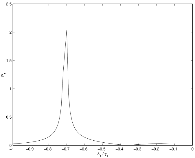
Figure 2: the relative fluctuation of $\chi_{1}(\omega_{1})$, for $\alpha^{2}=500$, $\gamma_{1}\gg\gamma_{3}$ and $\bar{\Omega}_{2}=g_{2}\sqrt{\bar{n}_{\alpha}+1}=\gamma_{1}/2$.

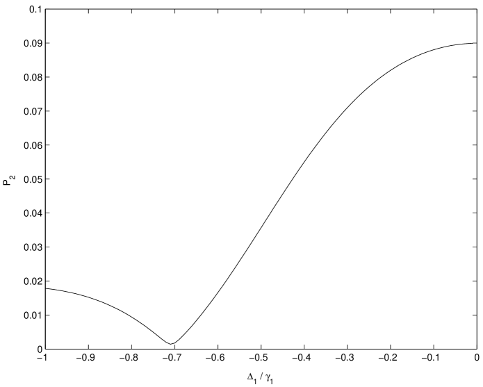
Figure 3: the relative fluctuation of $\chi_{2}(\omega_{1})$, for $\alpha^{2}=500$, $\gamma_{1}\gg\gamma_{3}$ and $\bar{\Omega}_{2}=g_{2}\sqrt{\bar{n}_{\alpha}+1}=\gamma_{1}/2$.

Noting that $P_{1}=\Delta\chi_{1}(\omega_{1})/{|\bar{\chi}_{1}(\omega_{1})|}$ and $P_{2}=\Delta\chi_{2}(\omega_{1})/{|\bar{\chi}_{2}(\omega_{1})|}$ are the relative fluctuation of $\chi_{1}(\omega_{1})$ and $\chi_{2}(\omega_{1})$ respectively. in Fig.2 and Fig.3, the relative fluctuation of $\chi_{1}(\omega_{1})$ and $\chi_{2}(\omega_{1})$ are plotted versus the detuning $\Delta_{1}$ in units of the atomic decay $\gamma_{1}$ respectively, for $\alpha^{2}=500$, $\gamma_{1}\gg\gamma_{3}$ and $\bar{\Omega}_{2}=g_{2}\sqrt{\bar{n}_{\alpha}+1}=\gamma_{1}/2$. It is seen that, around the zero detuning, for example, $\Delta_{1}\approx-0.1\gamma_{1}$. The relative fluctuation of $\chi_{1}(\omega_{1})$ is small ($\approx 4\%$), while that of $\chi_{2}(\omega_{1})$ is large ($\approx 9\%$). On the other hand, around the detuning $\Delta_{1}=-0.7$ the relative fluctuation of $\chi_{1}(\omega_{1})$ is large ($\approx 200\%$), while that of $\chi_{2}(\omega_{1})$ is small ($\approx 0.4\%$). Furthermore, the derivative of $\hat{\chi}_{1}(\omega_{1})$ is related to the group velocity for the probe laser pulse through

$$\hat{V}_{g}=c/{\left[1+(\omega_{1}/2)(\frac{{\mathrm{d}}\hat{\chi}_{1}}{{\mathrm{d}}\omega_{1}})\right]}$$ (22)

from which we can further numerically calculate the accompany fluctuation of the velocity. For example, on the zero detuning $\Delta_{1}=0$, we obtain $\bar{V}_{g}=10.02$ m/s, uncertainty $\Delta V_{g}=0.45$ m/s, and relative fluctuation $\Delta V_{g}/\bar{V}_{g}\approx 4.5\%$, while on the detuning $\Delta_{1}=0.16\gamma_{1}$, we obtain$\bar{V}_{g}=39.45$ m/s, uncertainty $\Delta V_{g}=27.90$ m/s, and relative fluctuation $\Delta V_{g}/\bar{V}_{g}\approx 70.7\%$.

The results above shows that the group velocity of the probe laser is not a certainty in the fully quantized model. Its uncertainty is a function of detuning $\Delta_{1}$. In what follows we shall give an approximate uncertainty relation between the phase operator of coupling laser and the group velocity, for the two-mode coherent state $|\alpha,\beta\!\!>$, as an approximation, we have

$$\hat{V}_{g}\approx\bar{V}_{g}(\bar{n}_{\alpha},\Delta_{1})+\frac{\partial{f(n_{2},\Delta_{1})}}{\partial{n_{2}}}|_{n_{2}=n_{\alpha}}(\hat{n}_{2}-\bar{n}_{\alpha})$$ (23)

where $f(n_{2},\Delta_{1})=c/{[1+(1/2)\frac{{\mathrm{d}}}{{\mathrm{d}}\omega_{1}}(\frac{g_{1}^{2}N(\Delta_{1}^{3}-g_{2}^{2}(n_{2}+1)\Delta_{1})}{(g_{2}^{2}(n_{2}+1)-\Delta_{1}^{2})^{2}+\gamma_{1}^{2}\Delta_{1}^{2}})]}$, and $\hat{n}_{2}=\hat{a}_{2}^{\dagger}\hat{a}_{2}$ is the particle number operators of the coupling laser modes and it satisfies the commutation relation[14]:

$$[\hat{n}_{2},\cos{\hat{\phi}}]=-i\sin{\hat{\phi}}$$ (24)

where $\cos{\hat{\phi}}$ is the phase operator of the coupling laser, then

$$[\hat{V}_{g},\cos{\hat{\phi}}]=-iF(n_{\alpha},\Delta_{1})\sin{\hat{\phi}}$$ (25)

where $F(n_{\alpha},\Delta_{1})=\frac{\partial{f(n_{2},\Delta_{1})}}{\partial{n_{2}}}|_{n_{2}=n_{\alpha}}$, from the uncertainty principle, we have

$$\langle\Delta\hat{V}_{g}\rangle\langle\Delta\cos{\hat{\phi}}\rangle\geq\frac{1}{2}|F(n_{\alpha},\Delta_{1})\langle\sin{\hat{\phi}}\rangle|$$ (26)

which turns out that the uncertainty of the group velocity is the function of $n_{\alpha}$ and $\Delta_{1}$.

As we have known that to decelerate and stop the input pulse, the strength of the coupling laser need to be modified from finite to zero [8, 9, 13], but when $\Omega_{2}$ is very small, we should treat the coupling laser as quantized. It is noticeable that if initially the coupling laser is much strong than the probe one, the coupling laser will be much stronger than the probe laser at all times(see Ref.[8]), which satisfies the condition of part (b) we discussed above.

(c) When both the probe and coupling lasers are very weak and have similar intensities, i.e., $\bar{n}_{\alpha}\sim\bar{n}_{\beta}$, from (4) we have $\tilde{\rho}_{bb}^{(0)}=\frac{\Omega_{2}^{2}}{\Omega^{2}}$ and $\tilde{\rho}_{cc}^{(0)}=\frac{\Omega_{1}^{2}}{\Omega^{2}}$, hence from the equation (11) the form of the density matrix element $\tilde{\rho}_{ab}$ can be followed:

$$\tilde{\rho}_{ab}=\frac{i\frac{\wp_{ab}}{2\hbar}\hat{E}_{1}(z)\rho_{bb}^{(0)}\left[(\gamma_{3}+i\Delta_{1})\gamma_{2}+g_{1}^{2}\hat{a}_{1}\hat{a}_{1}^{\dagger}\right]}{(\gamma_{1}+i\Delta_{1})(\gamma_{3}+i\Delta_{1})\gamma_{2}+\gamma_{2}g_{2}^{2}\hat{a}_{2}\hat{a}_{2}^{\dagger}+(\gamma_{1}+i\Delta_{1})g_{1}^{2}\hat{a}_{1}\hat{a}_{1}^{\dagger}}$$ (27)

and

$$\hat{\chi}(\omega_{1})=\frac{ig_{1}^{2}N\rho_{bb}^{(0)}\left[(\gamma_{3}+i\Delta_{1})\gamma_{2}+g_{1}^{2}\hat{a}_{1}\hat{a}_{1}^{\dagger}\right]}{\omega_{1}\left[(\gamma_{1}+i\Delta_{1})(\gamma_{3}+i\Delta_{1})\gamma_{2}+\gamma_{2}g_{2}^{2}\hat{a}_{2}\hat{a}_{2}^{\dagger}+(\gamma_{1}+i\Delta_{1})g_{1}^{2}\hat{a}_{1}\hat{a}_{1}^{\dagger}\right]}$$ (28)

From the above result we find that the susceptibility depends on the coupling laser as well as the probe laser when both of them are equally strong, which is similar to the result of KCW in Ref[11], but here the susceptibility is an operator and its value can be calculated on the Fock space just as the analysis in part(b).

3 Conclusion

We have developed a fully quantized model for EIT in which the decay rates are taken into account. In this model, to solve the evolution equation for density matrix, we separate the atom-system from the photon-system described by Fock-states and only calculate the density matrix of atom-system. By this means, the general form of susceptibility and group velocity of the probe laser we obtained are operators concerned with particle number operators of the probe and coupling laser modes. Their expectation value and fluctuation can be calculated on the Fock space. We have calculated the uncertainty of the group velocity numerically and give an approximate uncertainty relation between the phase operator of the coupling laser and the group velocity. When both the probe and coupling lasers are weak and have similar intensities, we find the susceptibility depends on the coupling laser as well as the probe laser. Considering the decay rates of various levels, we can make analysis of absorption of probe laser near resonance and calculate the fluctuation in both absorption and dispersion. We also discuss how the fully quantized model reduces to a semiclassical model when the mean photon numbers of the coupling laser is large.

This work is in part supported by NSF of China.

=0.8

=0.8

=0.8