Quantum Computing Without Entanglement 

Abstract

It is generally believed that entanglement is essential for quantum computing. We present here a few simple examples in which quantum computing without entanglement is better than anything classically achievable, in terms of the reliability of the outcome after a fixed number of oracle calls. Using a separable (that is, unentangled) $n$-qubit state, we show that the Deutsch-Jozsa problem and the Simon problem can be solved more reliably by a quantum computer than by the best possible classical algorithm, even probabilistic. We conclude that: (a) entanglement is not essential for quantum computing; and (b) some advantage of quantum algorithms over classical algorithms persists even when the quantum state contains an arbitrarily small amount of information—that is, even when the state is arbitrarily close to being totally mixed.

1 Introduction

Quantum computing is a new fascinating field of research in which the rules of quantum mechanics are used to solve various computing problems more efficiently than any classical algorithm could do [14, 11]. This has been rigourously demonstrated in oracle settings [2] and there is significant evidence that it is true in unrelativized cases as well [17]. The quantum unit of information is called the qubit. In addition to the “classical” states $|0\rangle$ and $|1\rangle$, a qubit can be in any superposition $|\psi\rangle=\alpha|0\rangle+\beta|1\rangle$, where $|\cdot\rangle$ is the standard Dirac notation for quantum states, and $\alpha$ and $\beta$ are complex numbers subject to $|\alpha|^{2}+|\beta|^{2}=1$. For instance, $|\pm\rangle=\raisebox{0.43057pt}[0.0pt][0.0pt]{\small$\textstyle\frac{1}{\sqrt{2}}$}\mbox{$|0\rangle$}\pm\raisebox{0.43057pt}[0.0pt][0.0pt]{\small$\textstyle\frac{1}{\sqrt{2}}$}\mbox{$|1\rangle$}$ and $|\pm_{i}\rangle=\raisebox{0.43057pt}[0.0pt][0.0pt]{\small$\textstyle\frac{1}{\sqrt{2}}$}\mbox{$|0\rangle$}\pm\raisebox{0.43057pt}[0.0pt][0.0pt]{\small$\textstyle\frac{i}{\sqrt{2}}$}\mbox{$|1\rangle$}$ are some specific pure states that we shall use later on. When $n$ qubits are used, their state can be in a superposition of all “classical” $n$-bit states, that is, $|\psi\rangle=\sum_{i=0}^{2^{n}-1}\alpha_{i}|i\rangle$, where $i$ is written in binary representation and $\sum_{i}|\alpha_{i}|^{2}=1$. These states are called pure states.

If qubits $|\psi\rangle$ and $|\varphi\rangle$ are in states $\alpha\mbox{$|0\rangle$}+\beta\mbox{$|1\rangle$}$ and $\gamma\mbox{$|0\rangle$}+\delta\mbox{$|1\rangle$}$, respectively, the state of a two-qubit system composed of those two qubits is given by their tensor product

$$|\psi\rangle\otimes|\varphi\rangle=\alpha\gamma\mbox{$|00\rangle$}+\alpha\delta\mbox{$|01\rangle$}+\beta\gamma\mbox{$|10\rangle$}+\beta\delta\mbox{$|11\rangle$}\,.$$ (1)

This notion generalizes in the obvious way to the tensor product of arbitrarily many quantum systems. Perhaps the most nonclassical aspect of quantum information processing stems from the fact that not all two-qubit states can be written in the form of Eq. (1). For instance, the states $|\Psi^{\pm}\rangle=\raisebox{0.43057pt}[0.0pt][0.0pt]{\small$\textstyle\frac{1}{\sqrt{2}}$}|01\rangle\pm\raisebox{0.43057pt}[0.0pt][0.0pt]{\small$\textstyle\frac{1}{\sqrt{2}}$}|10\rangle$ and $|\Phi^{\pm}\rangle=\raisebox{0.43057pt}[0.0pt][0.0pt]{\small$\textstyle\frac{1}{\sqrt{2}}$}|00\rangle\pm\raisebox{0.43057pt}[0.0pt][0.0pt]{\small$\textstyle\frac{1}{\sqrt{2}}$}|11\rangle$, known as the Bell states—or perhaps more appropriately the Braunstein-Mann-Revzen (BMR) states [5]—do not factor out as a tensor product. In general, state $a\mbox{$|00\rangle$}+b\mbox{$|01\rangle$}+c\mbox{$|10\rangle$}+d\mbox{$|11\rangle$}$ can be written in the form of Eq. (1) if and only if $ad=bc$. Multiple-qubits pure states that can be written as a tensor product of the individual qubits are said to be separable, or product states. Otherwise they are entangled.

When information is lacking about the state of a qubit, we say that this qubit is in a mixed state. This is described by a matrix $\rho=\sum_{j}p_{j}|\psi_{j}\rangle\langle\psi_{j}|$, called the density matrix, with $p_{j}$ being the probability of each (pure) state $|\psi_{j}\rangle$. The representation of $\rho$ as a sum is not unique. For instance, an equal mixture of $|\psi_{+}(\theta)\rangle=\cos\theta|0\rangle+\sin\theta|1\rangle$ and $|\psi_{-}(\theta)\rangle=\cos\theta|0\rangle-\sin\theta|1\rangle$ is written as $\rho_{\theta}=\frac{1}{2}|\psi_{+}(\theta)\rangle\langle\psi_{+}(\theta)|+\frac{1}{2}|\psi_{-}(\theta)\rangle\langle\psi_{-}(\theta)|$. Simple algebra shows that this is in fact exactly the same as $(\cos^{2}\theta)|0\rangle\langle 0|+(\sin^{2}\theta)|1\rangle\langle 1|$, which is in general an unequal mixture of $|0\rangle$ and $|1\rangle$. A quantum mixed state $\rho$ of several qubits is called a product state if it can be written as a tensor product of the states of the individual qubits, such as $\rho=\rho_{A}\otimes\rho_{B}$.

Recall that in the case of pure states, any product state is separable and any non-product state is entangled. The situation with mixed states is different—and more interesting—because there are separable states that are not product states. We say that a multiple-qubit mixed state is separable if it can be written as $\rho=\sum_{j}p_{j}|\psi_{j}\rangle\langle\psi_{j}|$ such that each of the $|\psi_{j}\rangle$ is a separable pure state. Equivalently, a mixed state $\rho$ is separable if it can be written in the form $\rho=\sum_{j}p_{j}\rho_{j}$ such that each of the $\rho_{j}$ is a product state.

The intuition behind this definition is that a state (pure or mixed) is separable if and only if it can be prepared in remote locations with the help of classical communication only. For instance, Alice and Bob can remotely prepare the separable bipartite state $\frac{1}{2}|01\rangle\langle 01|+\frac{1}{2}|10\rangle\langle 10|$ as follows. Alice tosses a fair coin and tells the outcome to Bob over a classical channel. If the coin came up heads, Alice and Bob prepare their qubits in states $|0\rangle$ and $|1\rangle$, respectively. But if the coin comes up tails, they prepare their qubits in states $|1\rangle$ and $|0\rangle$. Then, provided Alice and Bob forget the outcome of the coin, they are left with the desired state.

If a mixed state is not separable, then we say that it is entangled. Deciding if a mixed state is entangled or separable is not an easy task in the general case because its representation is not unique. For instance, the state $\frac{1}{2}|\Psi^{+}\rangle\langle\Psi^{+}|+\frac{1}{2}|\Psi^{-}\rangle\langle\Psi^{-}|$ is separable, despite being a mixture of two entangled pure states, because it can be written equivalently as $\frac{1}{2}|01\rangle\langle 01|+\frac{1}{2}|10\rangle\langle 10|$. As a more sophisticated example, a Werner state [19] $\chi=\lambda|\Psi^{-}\rangle\langle\Psi^{-}|+\frac{1-\lambda}{3}\left[\,|\Psi^{+}\rangle\langle\Psi^{+}|+|\Phi^{-}\rangle\langle\Phi^{-}|+|\Phi^{+}\rangle\langle\Phi^{+}|\,\right]$, which can also be written as

$$\chi=\varepsilon|\Psi^{-}\rangle\langle\Psi^{-}|+(1-\varepsilon)\,\textup{I}/4$$ (2)

with $\varepsilon=(4\lambda-1)/3$ and I a $4\times 4$ identity matrix, is entangled if and only if $\lambda>\frac{1}{2}$, or equivalently $\varepsilon>\frac{1}{3}$. For $\lambda=\frac{1}{4}$ ($\varepsilon=0$) the state is fully mixed, hence it contains no information. For $\lambda=\frac{1}{2}$ ($\varepsilon=\frac{1}{3}$) the state can be rewritten as

$$\textstyle\frac{1}{6}(|\Psi^{+}\rangle\langle\Psi^{+}|+|\Psi^{-}\rangle\langle\Psi^{-}|)+\frac{1}{6}(|\Phi^{-}\rangle\langle\Phi^{-}|+|\Psi^{-}\rangle\langle\Psi^{-}|)+\frac{1}{6}(|\Phi^{+}\rangle\langle\Phi^{+}|+|\Psi^{-}\rangle\langle\Psi^{-}|)\,,$$

which makes its separability immediately apparent because

$$\mbox{$|\Phi^{-}\rangle\langle\Phi^{-}|+|\Psi^{-}\rangle\langle\Psi^{-}|$}~{}=~{}\mbox{$|+-\rangle\langle+-|+|-+\rangle\langle-+|$}$$

and

$$\mbox{$|\Phi^{+}\rangle\langle\Phi^{+}|+|\Psi^{-}\rangle\langle\Psi^{-}|$}~{}=~{}\mbox{$|+_{i}-_{i}\rangle\langle+_{i}-_{i}|+|-_{i}+_{i}\rangle\langle-_{i}+_{i}|$}\,.$$

Note that, although separable, this state is far from being classical, as only a nontrivial mixture of states written in different bases exposes its separability.

Quantum computers can manipulate quantum information by means of unitary transformations [11, 14, 7]. In particular, they can work with superpositions. For instance, a single-qubit Walsh–Hadamard operation H transforms a qubit from $|0\rangle$ to $|+\rangle$ and from $|1\rangle$ to $|-\rangle$. When H is applied to a superposition such as $|+\rangle$, it follows by the linearity of quantum mechanics that the resulting state is $\frac{1}{2}((|0\rangle+|1\rangle)+(|0\rangle-|1\rangle))=|0\rangle$. This illustrates the phenomenon of destructive interference, by which component $|1\rangle$ of the state is erased. Consider now an $n$-qubit quantum register initialized to $|0^{n}\rangle$. Applying a Walsh–Hadamard transform to each of these qubits yields an equal superposition of all $n$-bit classical states:

$$|0^{n}\rangle\stackrel{{\scriptstyle\textsf{\scriptsize H}}}{{\longrightarrow}}\frac{1}{2^{n/2}}\sum_{x=0}^{2^{n}-1}|x\rangle\,.$$

Consider now a function $f:\{0,1\}^{n}\longrightarrow\{0,1\}$ that maps $n$-bit strings to a single bit. On a quantum computer, because unitary transformations are reversible, it is natural to implement it as a unitary transformation $U_{f}$ that maps $|x\rangle|b\rangle$ to $|x\rangle|b\oplus f(x)\rangle$, where $x$ is an $n$-bit string, $b$ is a single bit, and “$\oplus$” denotes the exclusive-or. Schematically,

$$|x\rangle|b\rangle\stackrel{{\scriptstyle U_{f}}}{{\longrightarrow}}|x\rangle|f(x)\oplus b\rangle\,.$$ (3)

The linearity of quantum mechanics gives rise to two important phenomena. (1) Quantum parallelism: we can compute $f$ on arbitrarily many classical inputs by a single application of $U_{f}$ to a suitable superposition:

$$\sum_{x}\alpha_{x}|x\rangle|b\rangle\stackrel{{\scriptstyle U_{f}}}{{\longrightarrow}}\sum_{x}\alpha_{x}|x\rangle|f(x)\oplus b\rangle\,.$$ (4)

When this is done, the additional output qubit may become entangled with the input register; (2) Phase kick-back: the outcome of $f$ can be recorded in the phase of the input register rather than being XOR-ed to the additional output qubit:

$$|x\rangle|-\rangle\stackrel{{\scriptstyle U_{f}}}{{\longrightarrow}}(-1)^{f(x)}|x\rangle|-\rangle\,;~{}~{}~{}\ \sum_{x}\alpha_{x}|x\rangle|-\rangle\stackrel{{\scriptstyle U_{f}}}{{\longrightarrow}}\sum_{x}\alpha_{x}(-1)^{f(x)}|x\rangle|-\rangle\,.$$ (5)

Much of the current interest in quantum computation was spurred by Peter Shor’s momentous discovery that quantum computers can in principle factor large numbers and extract discrete logarithms in polynomial time [17] and thus break much of contemporary cryptography, such as the RSA cryptosystem and the Diffie-Hellman public-key exchange. However, this does not provide a proven advantage of quantum computation because nobody knows for sure that these problems are genuinely hard for classical computers. On the other hand, it has been demonstrated that quantum computers can solve some problems exponentially faster than any classical computer provided the input is given as an oracle [8, 2], and even if we allow bounded errors [18]. In this model, some function $f:\{0,1\}^{n}\rightarrow\{0,1\}$ is given as a black-box, which means that the only way to obtain knowledge about $f$ is to query the black-box on chosen inputs. In the corresponding quantum oracle model, a function $f$ is provided by a black-box that applies unitary transformation $U_{f}$ to any chosen quantum state, as described by Eq. (3). The goal of the algorithm is to learn some property of the function.

A fundamental question is: Where does the surprising computational advantage provided by quantum mechanics come from? What is the nonclassical property of quantum mechanics that leads to such an advantage? Do superposition and interference provide the quantum advantage? Probably the most often heard answer is that the power of quantum computing comes from the use of entanglement, and indeed there are very strong arguments in favour of this belief. (See [12, 4, 13, 10, 15] for a discussion.)

We show in this paper that this common belief is wrong. To this effect, we present two simple examples in which quantum algorithms are better than classical algorithms even when no entanglement is present. Furthermore, we show that quantum algorithms can be better than classical algorithms even when the state of the computer is almost totally mixed—which means that it contains an arbitrarily small amount of information.

The most usual measure of efficiency for computer algorithms is the amount of time required to obtain the solution, as function of the input size. In oracle setting this usually means the number of queries needed to gain a predefined amount of information about the solution. Here, we fix a maximum number of oracle calls and we try to obtain as much Shannon information as possible about the correct answer. In this model, we analyse two famous problems due to Deutsch-Jozsa [8] and Simon [18]. We show that, when a single oracle query is performed, the probability to obtain the correct answer is better for the quantum algorithm than for the optimal classical algorithm, and that the information gained by that single query is higher. This is true even when no entanglement is ever present throughout the quantum computation and even when the state of the quantum computer is arbitrarily close to being totally mixed. The case of more than one query is left for future research, as well as the case of a fixed average number of queries rather than a fixed maximum number.

2 Pseudo-Pure States

To show that no entanglement occurs throughout our quantum computation, we use a special quantum state known as pseudo pure state (PPS) [9]. This state occurs naturally in the framework of Nuclear Magnetic Resonance (NMR) quantum computing [6], but the results presented in our paper are inherently interesting, regardless of the original NMR motivation. Consider any pure state $|\psi\rangle$ on $n$-qubits and some real number $0\leq\varepsilon\leq 1$. A pseudo-pure state has the following form:

$$\rho_{\rm PPS}^{\{n\}}\ \equiv\ \varepsilon|\psi\rangle\langle\psi|+(1-\varepsilon){\cal I}\,.$$ (6)

It is a mixture of pure state $|\psi\rangle$ with the totally mixed state ${\cal I}=\frac{1}{2^{n}}\textup{I}_{2^{n}}$ (where $\textup{I}_{2^{n}}$ denotes the identity matrix of order $2^{n}$). For example, the Werner state (2) is a special case of a PPS.

To understand why these states are called pseudo-pure, consider what happens if a unitary operation $U$ is performed on state $\rho=\rho_{\rm PPS}^{\{n\}}$ from Eq. 6.

Proposition 1

The purity parameter $\varepsilon$ of pseudo-pure states is conserved under unitary transformations.

Proof. Since $\rho\stackrel{{\scriptstyle U}}{{\rightarrow}}U\rho U^{\dagger}$ and $U{\cal I}U^{\dagger}={\cal I}$,

$$U\rho\,U^{\dagger}=\varepsilon U|\psi\rangle\langle\psi|U^{\dagger}+(1-\varepsilon)U{\cal I}U^{\dagger}=\varepsilon|\varphi\rangle\langle\varphi|+(1-\varepsilon){\cal I}\ ,$$

where $|\varphi\rangle=U|\psi\rangle$. In other words, unitary operations affect only the pure part of these states, leaving the totally mixed part unchanged and leaving the pure proportion $\varepsilon$ intact.  

The main interest of pseudo-pure states in our context comes from the fact that there exists some bias $\varepsilon$ below which these states are never entangled. The following theorem was originally proven in [4, Eq. (11)] but an easier proof was subsequently given in [16]:

Theorem 2

(Braunstein et al. [4]) For any number $n$ of qubits, a state $\rho_{\rm PPS}^{\{n\}}$ is separable whenever

$$\varepsilon<\frac{1}{1+2^{2n-1}}\,,$$ (7)

regardless of its pure part $|\psi\rangle$.

When $|\psi\rangle$ is entangled but $\rho_{\rm PPS}^{\{n\}}$ is separable, we say that the PPS exhibits pseudo-entanglement. (Please note that Eq. (7) is sufficient for separability but not necessary.) The key observation is provided by the Corollary below, whose proof follows directly from Theorem 2 and Proposition 1.

Corollary 3

Entanglement will never appear in a quantum unitary computation that starts in a separable PPS whose purity parameter $\varepsilon$ obeys Eq. (7). A final measurement in the computational basis will not make entanglement appear either.

3 The Deutsch-Jozsa Problem

The problem considered by Deutsch and Jozsa [8] was the following. We are given a function $f:\{0,1\}^{n}\rightarrow\{0,1\}$ in the form of an oracle (or a black-box), and we are promised that either this function is constant—$f(x)=f(y)$ for all $x$ and $y$—or that it is balanced—$f(x)=0$ on exactly half the $n$-bit strings $x$. Our task is to decide which is the case. Historically, this was the first problem ever discovered for which a quantum computer would have an exponential advantage over any classical computer, in terms of computing time, provided the correct answer must be given with certainty. In terms of the number of oracle calls, the advantage is in fact much better than exponential: a single oracle call (in which the input is given in superposition) suffices for a quantum computer to determine the answer with certainty, whereas no classical computer can be sure of the answer before it has asked $2^{n-1}+1$ questions. More to the point, no information at all can be derived from the answer to a single classical oracle call.

The quantum algorithm of Deutsch and Jozsa (DJ) solves this problem with a single query to the oracle by starting with state $|0^{n}\rangle\mbox{$|1\rangle$}$ and performing a Walsh–Hadamard transform on all $n+1$ qubits before and after the application of $U_{f}$. A measurement of the first $n$ qubits is made at the end (in the computational basis), yielding classical $n$-bit string $z$. By virtue of phase kickback, the initial Walsh–Hadamard transforms and the application of $U_{f}$ result in the following state:

$$|0^{n}\rangle|1\rangle \stackrel{{\scriptstyle\textsf{\scriptsize H}}}{{\longrightarrow}} \bigg{(}\frac{1}{2^{n/2}}\sum_{x}|x\rangle\bigg{)}|-\rangle\ \stackrel{{\scriptstyle U_{f}}}{{\longrightarrow}}\bigg{(}\frac{1}{2^{n/2}}\sum_{x}(-1)^{f(x)}|x\rangle\bigg{)}|-\rangle\ .$$ (8)

Then, if $f$ is constant, the final Walsh–Hadamard transforms revert the state back to $\pm|0^{n}\rangle|1\rangle$, in which the overall phase is $+$ if $f(x)=0$ for all $x$ and $-$ if $f(x)=1$ for all $x$. In either case, the result of the final measurement is necessarily $z=0$. On the other hand, if $f$ is balanced, the phase of half the $|x\rangle$ in Eq. (8) is $+$ and the phase of the other half is $-$. As a result, the amplitude of $|0^{n}\rangle$ is zero after the final Walsh–Hadamard transforms because each $|x\rangle$ is sent to $+|0^{n}\rangle/2^{n/2}+\cdots$ by those transforms. Therefore, the final measurement cannot produce $z=0$. It follows from the promise that if we obtain $z=0$ we can conclude that $f$ is constant and if we obtain $z\neq 0$ we can conclude that $f$ is balanced. Either way, the probability of success is 1 and the algorithm provides full information on the desired answer.

On the other hand, due to the special nature of the DJ problem, a single query does not change our probability of guessing correctly whether the function is balanced or constant. Therefore the following proposition holds:

Proposition 4

When restricted to a single DJ oracle call, a classical computer learns no information about the type of $f$.

In sharp contrast, the following Theorem shows the advantage of quantum computing even without entanglement.

Theorem 5

When restricted to a single DJ oracle call, a quantum computer whose state is never entangled can learn a positive amount of information about the type of $f$.

Proof. Starting with a PPS in which the pure part is $|0^{n}\rangle\mbox{$|1\rangle$}$ and its probability is $\varepsilon$, we can still follow the Deutsch-Jozsa strategy, but now it becomes a guessing game. We obtain the correct answer with different probabilities depending on whether $f$ is constant or balanced: If $f$ is constant, we obtain $z=0$ with probability

$$P(z=0\mid f\mbox{ is constant})=\varepsilon+(1-\varepsilon)/2^{n}$$

because we started with state $|0^{n}\rangle\mbox{$|1\rangle$}$ with probability $\varepsilon$, in which case the Deutsch-Jozsa algorithm is guaranteed to produce $z=0$ since $f$ is constant, or we started with a completely mixed state with complementary probability $1-\varepsilon$, in which case the Deutsch-Jozsa algorithm produces a completely random $z$ whose probability of being zero is $2^{-n}$. Similarly,

$$P(z\neq 0\mid f\mbox{ is constant})=\frac{2^{n}-1}{2^{n}}(1-\varepsilon)\,.$$

If $f$ is balanced we obtain a non-zero $z$ with probability

$$P(z\neq 0\mid f\mbox{ is balanced})=\varepsilon+\frac{2^{n}-1}{2^{n}}(1-\varepsilon)\,,$$

and $z=0$ is obtained with probability

$$P(z=0\mid f\mbox{ is balanced})=(1-\varepsilon)/2^{n}\,.$$

For all positive $\varepsilon$ and all $n$, we still observe an advantage over classical computation. In particular, this is true for $\varepsilon\leq 1/(1+2^{2n+1})$, in which case the state remains separable throughout the entire computation (Eq. (7) with $n+1$ qubits.)

Let the a priori probability of $f$ being constant be $p$ (and therefore the probability that it is balanced is $1-p$). The probability $p_{0}$ of obtaining $z=0$ is $\frac{1-\varepsilon}{2^{n}}+\varepsilon p.$ We would like to quantify the amount of information we gain about the function, given the outcome of the measurement. In order to do this, we calculate the mutual information between $X$ and $Y$, where $X$ is a random variable signifying whether $f$ is constant or balanced, and $Y$ is a random variable signifying whether $z=0$ or not. Let the entropy function of a probability $q$ be $h(q)\equiv-q\lg q-(1-q)\lg(1-q)$. Then, the information gained by a single quantum query is

$$I(X;Y)=h(p)-p_{0}h\left(\frac{p}{p_{0}}\left(\varepsilon+\frac{1-\varepsilon}{2^{n}}\right)\right)-(1-p_{0})h\left(\frac{p(1-\varepsilon)}{1-p_{0}}\left(1-\frac{1}{2^{n}}\right)\right)\,.$$

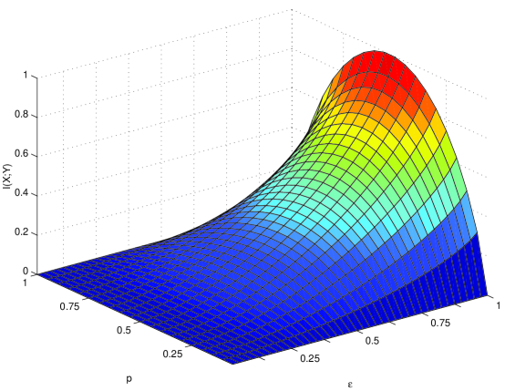
Figure 1: Information gained by one quantum Deutsch–Jozsa query: Always positive when $0<p<1$, even for extremely small positive $\varepsilon$

As shown by Figure 1, the mutual information is positive for every $\varepsilon>0$, unless $p=0$ or $p=1$. This is obviously more than the zero amount of information gained by a single classical query. For $p=1/2$ and very small $\varepsilon$ ($\varepsilon\ll\frac{1}{2^{n}}$) we obtain (cf. Appendix A) that

$$I(X;Y) = 1-p_{0}h\left(\frac{1}{2}+\frac{2^{n}\varepsilon}{4}+O(2^{n}\varepsilon^{2})\right)-(1-p_{0})h\left(\frac{1}{2}-\frac{\varepsilon}{1-4/2^{n}}+O(2^{n}\varepsilon^{2})\right)$$ (9)

$$= \frac{2^{2n}\varepsilon^{2}}{8(2^{n}-1)\ln 2}+O(2^{2n}\varepsilon^{3})>0.$$

 

For a specific example, consider $p=1/2$, $n=3$ and $\varepsilon=1/(1+2^{2n+1})=1/129$. In this case, we gain 0.0000972 bits of information.

We conclude that some information is gained even for separable PPSs, in contrast to the classical case where the mutual information is always zero. Furthermore, some information is gained even when $\varepsilon$ is arbitrarily small.

We can further improve the expected amount of information that is obtained by a single call to the oracle if we measure the $(n+1)$st qubit and take it into account. Indeed, this qubit should be $|1\rangle$ if the contribution comes from the pure part. Therefore, if that extra bit is $|0\rangle$, which happens with probability $(1-\varepsilon)/2$, we know that the PPS contributes the fully mixed part, hence no useful information is provided by $z$ and we are no better than in the classical case. However, knowing that you don’t know something is better than not knowing at all, because it makes the other case more revealing! Indeed, when that extra bit is $|1\rangle$, which happens with probability $(1+\varepsilon)/2$, the probability of the pure part is enlarged from $\varepsilon$ to $\hat{\varepsilon}=2\varepsilon/(1+\varepsilon)$, and the probability of the mixed part is reduced from $1-\varepsilon$ to $1-\hat{\varepsilon}=(1-\varepsilon)/(1+\varepsilon)$. The probability of $z=0$ changes to $\hat{p}_{0}=\frac{1-\hat{\varepsilon}}{2^{n}}+\hat{\varepsilon}p,$ and mutual information to

$$I(X;Y) = \frac{1+\varepsilon}{2}\left[h(p)-\hat{p}_{0}h\left(\frac{p}{\hat{p_{0}}}\left(\hat{\varepsilon}+\frac{1-\hat{\varepsilon}}{2^{n}}\right)\right)-(1-\hat{p}_{0})h\left(\frac{p(1-\hat{\varepsilon})}{1-\hat{p_{0}}}\left(1-\frac{1}{2^{n}}\right)\right)\right]$$

which, for $$p=1/2 \varepsilon$$ and very small , gives

$$I(X;Y) = \frac{2^{2n}\varepsilon^{2}}{4(2^{n}-1)\ln 2}+O(2^{2n}\varepsilon^{3})>0\,.$$

This is essentially twice as much information as in Eq. (9). For the specific example of $p=1/2$, $n=3$ and $\varepsilon=1/129$, this is 0.000189 bits of information.

4 The Simon Problem

An oracle calculates a function $f(x)$ from $n$ bits to $n$ bits. We are promised that $f$ is a two-to-one function, so that for any $x$ there exists a unique $y\mbox{}\neq x$ such that $f(x)=f(y)$. Furthermore, we are promised the existence of an $s\neq 0$ such that $f(x)=f(y)$ for $x\neq y$ if and only if $y=x\oplus s$, (where $\oplus$ is the bitwise exclusive-or operator). The goal is to find $s$, while minimizing the number of times $f$ is calculated.

Classically, even if one calls function $f$ exponentially many times, say $2^{n/4}$ times, the probability of finding $s$ is still exponentially small with $n$, that is less than $2^{-n/2}$. However, there exists a quantum algorithm that requires only $O(n)$ computations of $f$. The algorithm, due to Simon [18], is initialized with $|0^{n}\rangle|0^{n}\rangle$. It performs a Walsh–Hadamard transform on the first register and calculates $f$ for all inputs to obtain

$$|0^{n}\rangle|0^{n}\rangle \stackrel{{\scriptstyle\textsf{\scriptsize H}}}{{\longrightarrow}} \frac{1}{2^{n/2}}\sum_{x}|x\rangle|0^{n}\rangle\stackrel{{\scriptstyle U_{f}}}{{\longrightarrow}}\frac{1}{2^{n/2}}\sum_{x}|x\rangle|f(x)\rangle\,,$$ (10)

which can be written as

$$= \frac{1}{2^{n/2}}\sum_{x<x\oplus s}\left(|x\rangle+|x\oplus s\rangle\right)|f(x)\rangle\ .$$

Then, the Walsh–Hadamard transform is performed again on the first register (the one holding the superposition of all $|x\rangle$), which produces state

$$\frac{1}{2^{n}}\sum_{x<x\oplus s}\sum_{j}\left((-1)^{j\cdot x}+(-1)^{j\cdot x\oplus j\cdot s}\right)|j\rangle|f(x)\rangle\,,$$

where ‘$\cdot$’ is the inner product modulo 2 of the binary strings of $j$ and $s$. Finally the first register is measured. Notice that the outcome $j$ is guaranteed to be orthogonal to $s$ ($j\cdot s=0$) since otherwise $|j\rangle$’s amplitude $(-1)^{j\cdot x}\left(1+(-1)^{j\cdot s}\right)$ is zero. After an expected number of such queries in $O(n)$, one obtains $n$ linearly independent $j$s that uniquely define $s$.

Let $S$ be the random variable that describes parameter $s$, and $J$ be a random variable that describes the outcome of a single measurement. We would like to quantify how much information about $S$ is gained by a single query. Assuming that $S$ is distributed uniformly in the range $[1\,.\,.\,2^{n}-1]$, its entropy before the first query is $H(S)=\lg(2^{n}-1)\approx n$. In the classical case, a single evaluation of $f$ gives no information about $S$: the value of $f(x)$ on any specific $x$ says nothing about its value in different places, and therefore nothing about $s$. However, in the case of the quantum algorithm, we are assured that $s$ and $j$ are orthogonal. If the measured $j$ is zero, $s$ could still be any one of the $2^{n}-1$ non-zero values and no information is gained. But in the overwhelmingly more probable case that $j$ is non-zero, only $2^{n-1}-1$ values for $s$ are still possible. Thus, given the outcome of the measurement, the entropy of $S$ drops to approximately $n-1$ bits and the expected information gain is nearly one bit (See Appendix B for a detailed calculation). More formally, based on the conditional probability

$$P(J=j\mid S=s)=\left\{\begin{array}[]{ll}\frac{2}{2^{n}}&\mbox{if }j\cdot s=0\\[4.30554pt] 0&\mbox{if }j\cdot s=1\,,\end{array}\right.$$

it follows that the conditional entropy $H(J\mid S=s)=n-1$, which does not depend on the specific $s$ and therefore $H(J|S)=n-1$ as well. In order to find the a priori entropy of $J$, we calculate its marginal probability

$$P(J=j) = \sum_{s}P(s)P(j|s)$$

$$= \left\{\begin{array}[]{ll}\frac{1-\frac{2}{2^{n}}}{2^{n}-1}&\mbox{if }j\neq 0\\[4.30554pt] \frac{2}{2^{n}}&\mbox{if }j=0\,.\end{array}\right.$$

Thus,

$$H(J)=-\sum_{j}P(J=j)\lg P(J=j) = -\left(1-\frac{2}{2^{n}}\right)\lg\frac{1-\frac{2}{2^{n}}}{2^{n}-1}-\frac{2}{2^{n}}\lg\frac{2}{2^{n}}$$

$$= \left(1-\frac{2}{2^{n}}\right)\left(n+\lg\frac{2^{n}-1}{2^{n}-2}\right)+\frac{n-1}{2^{n-1}}$$

and the mutual information

$$I(S;J)=1-\frac{2-(2^{n}-2)\lg{\frac{2^{n}-1}{2^{n}-2}}}{2^{n}}=1-O(2^{-n})$$

is almost one bit.

\psfrag{epsilon}{$\varepsilon$}\includegraphics[width=289.07999pt]{simoninfo.eps}

Figure 2: Information gained by one quantum Simon query (here for $n=10$): Always positive, even for extremely small positive $\varepsilon$.

In contrast, a single query to a classical oracle provides no information about $s$.

Proposition 6

When restricted to a single oracle call, a classical computer learns no information about Simon’s parameter $s$.

Again in sharp contrast, the following Theorem shows the advantage of quantum computing without entanglement, compared to classical computing.

Theorem 7

When restricted to a single oracle call, a quantum computer whose state is never entangled can learn a positive amount of information about Simon’s parameter $s$.

Proof. Starting with a PPS in which the pure part is $|0^{n}\rangle|0^{n}\rangle$, and its probability is $\varepsilon$, the acquired $j$ is no longer guaranteed to be orthogonal to $s$. In fact, an orthogonal $j$ is obtained with probability $\frac{1+\varepsilon}{2}$ only. For any value of $S$, the conditional distribution of $J$ is

$$P(J=j\mid S=s)=\left\{\begin{array}[]{ll}\frac{1+\varepsilon}{2^{n}}&\mbox{if }j\cdot s=0\\[4.30554pt] \frac{1-\varepsilon}{2^{n}}&\mbox{if }j\cdot s=1\end{array}\right.$$

from which we calculate (see Appendix B) that the information gained about $S$ given the value of $J$ is

$$I(S;J)=-\left(1-\frac{1+\varepsilon}{2^{n}}\right)\lg\frac{1-\frac{1+\varepsilon}{2^{n}}}{2^{n}-1}+\left(2^{n-1}-1\right)\frac{1+\varepsilon}{2^{n}}\lg\frac{1+\varepsilon}{2^{n}}+\frac{1-\varepsilon}{2}\lg\left(\frac{1-\varepsilon}{2^{n}}\right).$$

As shown in Figure 2, the amount of information is larger than the classical zero for every $\varepsilon>0$.  

This theorem is true even for $\varepsilon$ as small as $1/(1+2^{2(2n)-1})$, in which case the state of the computer is never entangled throughout the computation by virtue of Corollary 3. For example, when $n=3$ and $\varepsilon=1/(1+2^{4\cdot 3-1})=1/2049$, we gain $147\times 10^{-9}$ bits of information.

5 Conclusions and Directions for Further Research

We have shown that quantum computing without entanglement is more powerful than classical computing. We achieved this result by using two well-known problems due to Deutsch-Jozsa and to Simon, and by comparing quantum-without-entanglement to classical behaviour. Our measure of performance was the amount of Shannon information that can be obtained when a single oracle query is allowed.

In the paper [4] that gave us Theorem 2, Braunstein, Caves, Jozsa, Linden, Popescu and Schack claimed that “…current NMR experiments should be considered as simulations of quantum computation rather than true quantum computation, since no entanglement appears in the physical states at any stage of the process” . Much to the contrary, we showed here that pseudo-entanglement is sufficient to beat all possible classical algorithms, which proves our point since pseudo-entangled states are not entangled! In conclusion, a few final remarks are in order.

• The quantum advantage that we have found is negligible (exponentially small). A much better advantage might be obtained by increasing $\varepsilon$ and investigating the separability of the specific states obtained throughout the unitary evolution of the algorithms.

• The case of more than one query is left for a future research.

• The case of a fixed average number of oracle calls, rather than a fixed maximum number of oracle calls, is also left for future research. Indeed, it was pointed out by Jozsa that a classical strategy can easily outperform our unentangled quantum strategy when solving the Deutsch-Jozsa problem if we restrict the number of oracle calls to be 1 on the average. For this, the classical computer tosses a coin. With probability $\mbox{}^{1}\!/_{2}$, it does not query the oracle at all and learns no information. But otherwise, also with probability $\mbox{}^{1}\!/_{2}$, it queries the oracle twice on random inputs and learns full information—that the function is balanced—if it obtains two distinct outputs. This happens with overall probability $\mbox{}^{1}\!/_{8}$ if the a priori probability of the function being balanced is $\mbox{}^{1}\!/_{2}$, which is much better than the exponentially small amount of information gleaned from our unentangled quantum strategy after one oracle call.

• What is the connection between this work and quantum communication complexity? (A survey of this topic can be found in [3].) Could quantum communication have an advantage over classical communication even when entanglement is not used?

Let us mention two papers that appear at first to contradict our results: Jozsa and Linden [12] showed that for a large class of computational problems, entanglement is required in order to achieve an exponential advantage over classical computation. Ambainis et al. [1] showed that quantum computation with a certain mixed state, other than the pseudo-pure state used by us, has no advantage over classical computation. But obviously, there is no real contradiction between our paper and these important results. We provide a case in which there exists a positive advantage of unentangled quantum computation over classical computation.

APPENDICES

Appendix A Details for the Deutsch-Jozsa Problem

The following two diagrams describe the probability that zero (or non-zero) is measured, given a constant (or balanced) function, in the pure and the totally mixed cases.

Figure 3: Pure initial state

Figure 4: Totally mixed initial state

The case of pseudo-pure initial state is the weighted sum of the previous cases.

Figure 5: Pseudo-pure initial state

The details of the pseudo-pure case are summarized in the joint probability table 1 below.

$X$	$y$=zero	$y$=non-zero
const.	$\raisebox{5.69054pt}{\rule[-14.22636pt]{0.0pt}{25.60747pt}}p\left(\varepsilon+\frac{1-\varepsilon}{2^{n}}\right)$	$p(1-\varepsilon)(1-\frac{1}{2^{n}})$
bal.	$\raisebox{5.69054pt}{\rule[-14.22636pt]{0.0pt}{17.07164pt}}(1-p)\frac{1-\varepsilon}{2^{n}}$	$(1-p)(1-\frac{1-\varepsilon}{2^{n}})$
$P(Y\mbox{=}y)$	$p_{0}=p\varepsilon+\frac{1-\varepsilon}{2^{n}}$	$1-p_{0}$

Table 1: Joint probability of function type ($X$) and measurement ($Y$)

The marginal probability of $Y$ and $X$ may be calculated from that table, and using Bayes rule, $P(X|Y)=\frac{P(Y|X)P(X)}{P(Y)}$, we find the conditional probabilities

$$P(X\mbox{=const}\mid Y\mbox{=zero}) = \frac{p}{p_{0}}\left(\varepsilon+\frac{1-\varepsilon}{2^{n}}\right)$$

and

$$P(X\mbox{=const}\mid Y\mbox{=nonzero}) \!\!= \!\!\frac{p(1-\varepsilon)}{1-p_{0}}\left(1-\frac{1}{2^{n}}\right)$$

where $p_{0}=P(Y\mbox{=zero})=p\varepsilon+\frac{1-\varepsilon}{2^{n}}$. The conditional entropy is

$$H(X|Y) = \sum_{y}P(Y=y)h(P(X\mbox{=const}\mid Y=y))$$

$$= p_{0}h\left(\frac{p}{p_{0}}\left(\varepsilon+\frac{1-\varepsilon}{2^{n}}\right)\right)+(1-p_{0})h\left(\frac{p(1-\varepsilon)}{1-p_{0}}\left(1-\frac{1}{2^{n}}\right)\right),$$

and the mutual information is, therefore,

$$I(X;Y) = H(X)-H(X|Y)$$

$$= h(p)-p_{0}h\left(\frac{p}{p_{0}}\left(\varepsilon+\frac{1-\varepsilon}{2^{n}}\right)\right)-(1-p_{0})h\left(\frac{p(1-\varepsilon)}{1-p_{0}}\left(1-\frac{1}{2^{n}}\right)\right).$$

For $p=\frac{1}{2}$ this reduces into

$$1-\frac{1+\varepsilon\,\left(2^{n-1}-1\right)}{2^{n}}\,h\left(\frac{1+\varepsilon\,\left({2^{n}}-1\right)}{2\,\left(1+\varepsilon\,\left(2^{n-1}-1\right)\right)}\right)$$

$$~{}~{}~{}-\frac{{2^{n}}-1-\varepsilon\,\left(2^{n-1}-1\right)}{2^{n}}\,h\left(\frac{\left(\varepsilon-1\right)\,\left({2^{n}}-1\right)}{2\,\left(1+\varepsilon\,\left(2^{n-1}-1\right)-{2^{n}}\right)}\right)$$

and for very small $\varepsilon$ ($\varepsilon\ll\frac{1}{2^{n}}$) , using that fact that $h(1/2+x)=1-\frac{2\,x^{2}}{\ln 2}+O(x^{4})$, this expression may be approximated by

$$I(X;Y) = 1-p_{0}h\left(\frac{1}{2}+\frac{2^{n}\varepsilon}{4}+O(2^{n}\varepsilon^{2})\right)-(1-p_{0})h\left(\frac{1}{2}-\frac{\varepsilon}{1-4/2^{n}}+O(2^{n}\varepsilon^{2})\right)$$

$$= \frac{2^{2n}\varepsilon^{2}}{8(2^{n}-1)\ln 2}+O(2^{2n}\varepsilon^{3})>0.$$

Appendix B Details for the Simon Problem

Let $S$ be a random variable that represents the sought-after parameter of Simon’s function, so that $\forall x:f(x)=f(x\oplus s)$. Throughout this discussion, we assume that $S$ is distributed uniformly in the range $[1\,.\,.\,2^{n}-1]$. Given that $S=s$, and starting with a PPS whose purity is $\varepsilon$, one may find the distribution of the measurement after a single query. With probability $\varepsilon$ we have started with the pure part and measured a $j$ that is orthogonal to $s$. With probability $1-\varepsilon$ we have started with the totally mixed state and measured a random $j$. Thus for $j$ so that $j\cdot s=0$, $P(J=j\mid S=s)=\varepsilon\frac{2}{2^{n}}+(1-\varepsilon)/{2^{n}},$ and for $j$ so that $j\cdot s=1$, $P(J=j\mid S=s)=(1-\varepsilon)/{2^{n}}.$ Putting this together,

$$P(J=j\mid S=s)=\left\{\begin{array}[]{ll}\frac{1+\varepsilon}{2^{n}}&\mbox{if }j\cdot s=0\\[4.30554pt] \frac{1-\varepsilon}{2^{n}}&\mbox{if }j\cdot s=1\,.\end{array}\right.$$

The marginal probability of $J$ for any $j\neq 0$ is

$$P(J=j) = \sum_{s}P(s)P(j|s)$$

$$= \frac{1}{2^{n}-1}\left(\sum_{s\perp j}P(j|s)+\sum_{s\not\perp j}P(j|s)\right)$$

$$= \frac{(2^{n-1}-1)\frac{1+\varepsilon}{2^{n}}+2^{n-1}\frac{1-\varepsilon}{2^{n}}}{2^{n}-1}$$

$$= \frac{1-\frac{1+\varepsilon}{2^{n}}}{2^{n}-1},$$

while for $J=0$, all values of $s$ are orthogonal, and

$$P(J=0) = \sum_{s}P(s)P(J=0|s)$$

$$= \frac{1}{2^{n}-1}\sum_{s\perp j}P(J=0|s)$$

$$= \frac{1}{2^{n}-1}(2^{n}-1)\frac{1+\varepsilon}{2^{n}}$$

$$= \frac{1+\varepsilon}{2^{n}}.$$

By definition, the entropy of the random variable $J$ is

$$H(J) = -\sum_{j}P(J=j)\lg P(J=j)$$

$$= -\left(1-\frac{1+\varepsilon}{2^{n}}\right)\lg\frac{1-\frac{1+\varepsilon}{2^{n}}}{2^{n}-1}-\frac{1+\varepsilon}{2^{n}}\lg\frac{1+\varepsilon}{2^{n}},$$

and the conditional entropy of $J$ given $S=s$ is

$$H(J\mid S=s) = -\sum_{j}P(J=j\mid S=s)\lg P(J=j\mid S=s)$$

$$= -2^{n-1}\frac{1+\varepsilon}{2^{n}}\lg\left(\frac{1+\varepsilon}{2^{n}}\right)-2^{n-1}\frac{1-\varepsilon}{2^{n}}\lg\left(\frac{1-\varepsilon}{2^{n}}\right)$$

$$= -\frac{1+\varepsilon}{2}\lg\left(\frac{1+\varepsilon}{2^{n}}\right)-\frac{1-\varepsilon}{2}\lg\left(\frac{1-\varepsilon}{2^{n}}\right).$$

Since Eq. (B) is independent of the specific value $s$, it also equals to $H(J|S)$, which is $\sum_{s}P(S=s)H(J\mid S=s)$. Finally, the amount of knowledge about $S$ that is gained by knowing $J$ is their mutual information:

$$I(S;J) = I(J;S)~{}=~{}H(J)-H(J|S)$$

$$= -\left(1-\frac{1+\varepsilon}{2^{n}}\right)\lg\frac{1-\frac{1+\varepsilon}{2^{n}}}{2^{n}-1}+\left(2^{n-1}-1\right)\frac{1+\varepsilon}{2^{n}}\lg\frac{1+\varepsilon}{2^{n}}+\frac{1-\varepsilon}{2}\lg\left(\frac{1-\varepsilon}{2^{n}}\right).$$

Notice the two extremes: in the pure case ($\varepsilon=1$), $I(S;J)=1-O(2^{-n})$ and in the totally mixed case ($\varepsilon=0$), $I(S;J)=0$. Finally, it can be shown that for small $\varepsilon$

$$I(S;J)=\frac{(2^{n}-2)\varepsilon^{2}}{2(2^{n}-1)\ln 2}+O(\varepsilon^{3})\,.$$

References

- [1] A. Ambainis, L. J. Schulman and U. V. Vazirani, “Computing with Highly Mixed States”, Proceedings of the 32nd Annual ACM Symposium on the Theory of Computing, 697–704 (2000).
- [2] A. Berthiaume and G. Brassard, “Oracle Quantum Computing”, Journal of Modern Optics 41(12), 2521–2535 (1994).
- [3] G. Brassard, “Quantum Communication Complexity”, Foundations of Physics, to appear (2003).
- [4] S. L. Braunstein, C. M. Caves, R. Jozsa, N. Linden, S. Popescu and R. Schack, “Separability of Very Noisy Mixed States and Implications for NMR Quantum Computing”, Physical Review Letters 83, 1054–1057 (1999).
- [5] S. L. Braunstein, A. Mann and M. Revzen, “Maximal Violation of Bell Inequalities for Mixed States”, Physical Review Letters 68, 3259–3261 (1992).
- [6] D. G. Cory, A. F. Fahmy and T. F. Havel, “Ensemble Quantum Computing by Nuclear Magnetic Resonance Spectroscopy”, Proceedings of the US National Academy of Sciences 94, 1634–1639 (1997).
- [7] D. Deutsch, “Quantum Computational Networks”, Proceedings of the Royal Society of London A425, 73–90 (1989).
- [8] D. Deutsch and R. Jozsa, “Rapid Solution of Problems by Quantum Computation”, Proceedings of the Royal Society of London A439, 553–558 (1992).
- [9] N. A. Gershenfeld and I. L. Chuang, “Bulk Spin-Resonance Quantum Computation”, Science 275, 350–356 (1997).
- [10] A. Ekert and R. Jozsa, “Quantum Algorithms: Entanglement Enhanced Information Processing”, Philosophical Transactions of the Royal Society of London A356, 1779–1782 (1998).
- [11] J. Gruska, Quantum Computing, McGraw-Hill, London, 1999.
- [12] R. Jozsa and N. Linden, “On the Role of Entanglement in Quantum Computational Speed-up”, arXiv:quant-ph/0201143, 2002.
- [13] N. Linden and S. Popescu, “Good Dynamics versus Bad Kinematics: Is Entanglement Needed for Quantum Computation?”, Physical Review Letters 87, 047901 (2001).
- [14] M. A. Nielsen and I. L. Chuang, Quantum Computation and Quantum Information, Cambridge University Press, 2000.
- [15] R. Schack and C. M. Caves, “Classical Model for Bulk-Ensemble NMR Quantum Computation”, Physical Review A 60, 4354–4362 (1999).
- [16] R. Schack and C. M. Caves, “Explicit Product Ensembles for Separable Quantum States”, Journal of Modern Optics 47, 387–399 (2000).
- [17] P. W. Shor, “Polynomial-Time Algorithms for Prime Factorization and Discrete Logarithms on a Quantum Computer”, SIAM Journal on Computing 26, 1484–1509 (1997).
- [18] D. R. Simon, “On the Power of Quantum Computation” SIAM Journal on Computing 26, 1474–1483 (1997).
- [19] R. F. Werner, “Quantum States With Einstein-Podolsky-Rosen Correlations Admitting a Hidden-Variable Model”, Physical Review A 40(8), 4277–4281 (1989).