Transient dynamics of Light propagation in EIT medium and hidden symmetry of multi-bit quantum memory

Abstract

We investigate the transient phenomenon or property of the propagation of an optical probe field in a medium consisting of many $\Lambda$-type three-level atoms coupled to this probe field and an classical driven field. We observe a hidden symmetry and obtain an exact solution for this light propagation problem by means of the spectral generating method. This solution enlightens us to propose a practical protocol implementing the quantum memory robust for quantum decoherence in a crystal. As an transient dynamic process this solution also manifests an exotic result that a wave-packet of light will split into three packets propagating at different group velocities. It is argued that ”super-luminal group velocity” and ”sub-luminal group velocity” can be observed simultaneously in the same system. This interesting phenomenon is expected to be demonstrated experimentally.

]

I Introduction

The recent experiments [3, 4] have demonstrated many exotic natures of light pulse propagation in the solid and gas systems with electromagnetically induced transparency (EIT) [5], such as the phenomena of ”super-luminal group velocity” and ”sub-luminal group velocity”. Physically they reflect the quantum coherence effects to correlate the quantum fluctuations [6]. The concepts of atomic coherence and interference have also been applied to lasing without inversion [7] and the enhancement of linear or nonlinear susceptibilities [8, 9]. At present the sub-luminal phenomena including the light stopping in an atomic medium have been extensively studied from various points of view [10]. The recent experiments have also shown the ultra-slow group velocity of light in the solid state systems, such as 3-mm thick crystal of $Y_{2}SiO_{5}$ [11]. Most recently, it is found that when a few rubidium atoms are loaded into high-Q optical micro-cavity, the ”super-luminal” and ”sub-luminal” phenomena can be observed in a refined version of the above mentioned experiments [12].

With possible applications in quantum information field developed in the past ten years [13], some studies on the sub-luminal problem are closely associated with an ideal and reversible transfer technique for the quantum state between light and metastable collective states of matter [14]. Theoretically, the basic idea is based on the control of light propagation in a coherently driven 3-level atomic medium. The exciting fact that the group velocity is adiabatically reduced to zero [14] means the possibility of proposing a more practical protocol to store and transfer the quantum information of photons in the collective excitations in an ensemble of $\Lambda$-type 3-level atoms [15, 16]. This may open up an interesting prospective for quantum information processing. The studies show that the excitations of matter coupled by light are more stable under some circumstances and thus form the so-called ”dark-state polaritons”.  Physically speaking, this is the essence of the problem. Extended to the multi-atom case, the above idea about adiabatic transfer of the state of a single photon into that of an individual atom [17] provides a conceptually simplest approach for the implementation of the quantum memory of photon information. Technically, this approach combines the enhancement of the absorption cross section in multi-atom systems with dissipation-free adiabatic passage techniques. In addition, this significant investigation motivates the protocol for long distance quantum communication [23] based on atomic ensemble.

Most recently we have deeply investigated the robustness of this kind of quantum memory [24]. To avoid the spatial-motion induced decoherence in an ensemble of free atoms, we have naturally proposed a protocol that each $\Lambda$-type atom is fixed on a lattice site of a crystal [19]. As quantum memories robust for the spatial-motion induced decoherence, the quasi-spin wave collective excitation of many $\Lambda$-type atoms forms a two-mode exciton system with a dynamic symmetry (or a hidden symmetry) depicted by the semi-direct product algebra $SU(2)\overline{\otimes}h_{2}$ ($h_{2}$ is an algebra of two mode boson operator). Physically, this hidden symmetry guarantees the stable spectral structure of such dressed two-mode exciton system while its decoherence implies a symmetry breaking. If one only considers quantum memory, one can focus on the case of single mode light field. However, if one considers the propagation of light pulse in this EIT medium, it is then necessary to concern the multi-mode light field since a light pulse can be understood as a superposition of the components of different frequencies. The aim of the present and subsequent papers is to analyze the transient phenomenon or property of the light propagation in this EIT medium, especially to emphasize the role of the generalized hidden symmetry.

In this paper, our proposed system still consists of the quasi-spin wave collective excitation of many $\Lambda$-type 3-level subsystems as in ref.[19]. The meta-stable state still interacts with an exactly resonant classical field, but the approximately resonant quantized light field, which couples to the transition between the excited state and the relative ground state, is no longer of single mode. We will prove that, in the large $N$ limit, one needs to introduce a pair of exciton operators for each mode of quantized light field. These realize the infinite boson algebra local in the mode space (or the frequency domain), but the collective quasi-spin operators intertwining between the meta-stable states and the excited ones generate a single global $SU(2)$ algebra. With the help of this hidden symmetry and the corresponding spectral generating algebra method, we exactly obtain the dressed spectra of the total system formed by the infinite two-mode excitons coupling to a multi-mode quantized electromagnetic field in the large $N$ limit. The exact solutions for the eigen-states obtained in this way also include the multi-mode dark states extrapolating from photon to one mode quasi-spin wave exciton. Actually, these dressed states describe the polaritons only coupling a quasi-spin wave exciton to a photon for some special case. With the EIT mechanism the external classical field can be artificially manipulated to change the dispersion properties of the quasi-spin wave excitonic medium dramatically so that the quantized probing light can propagate in exotic ways. In this way the quantum information can be coherently stored and transferred among the multi-mode cavity photon and the multi-mode exciton system. Our studies in this paper are substantially related to the hidden symmetry and its breaking. The hidden symmetry leads to an exact class of solutions for the light propagation problem, showing that a wave-packet of light will split into three wave-packets which propagate at different group velocities, namely, the ”super-luminal group velocity”, the ”sub-luminal group velocity” and the usual light group velocity.

II Collective Excitation of Three-Level Medium

We consider the transient process for the weak light propagation in a medium consisting of many three-level subsystems. It can be an ensemble of $N$ free $\Lambda$-type atoms, or a crystal with $N$ lattice sites attached by $N$ $\Lambda$-type subspaces. In recent years, the similar exciton system in a crystal slab with spatially fixed ”two-level atoms” has been extensively discussed with the emphasis on fluorescence process and relevant quantum decoherence problem [18],[20].

As shown in Fig. 1, the $\Lambda$-type subsystem possesses an excited state $|a\rangle$, a ground state $|b\rangle$ and a meta-stable state $|c\rangle$. The transition frequency $\omega_{ac}$ from $|a\rangle$ to $|c\rangle$ of each atom is resonantly driven by a classical field of Rabi-frequency $\Omega$. The transition frequency $\omega_{ab}$ from $|a\rangle$ to $|b\rangle$ is coupled to a multi-mode quantized field with the annihilation operator $a_{k}$, and the coupling constant $g_{k}$ for the optical mode of wave vectors ${\bf k}$. Strictly speaking, a multi-mode field can’t be resonantly coupled to an atomic transition since it is a superposition of many components of different frequencies. We should emphasize here that we only consider the case that the quantized field is a Gaussian wave packet in the frequency domain and the center frequency $\omega_{0}$ just equals $\omega_{ab}$. When the frequency width of the wave packet is very small compared with $\omega_{0}$ ($\Delta\omega\ll\omega_{0}$), from the viewpoint of approximation it is reasonable to assume that the multi-mode quantized field couples resonantly to the atomic transition from $|a\rangle$ to $|b\rangle$. Therefore, the interaction Hamiltonian of total system reads

$$H = \sum_{{\bf j}=1}^{N}\sum_{k}g_{k}a_{k}\exp(i{\bf k}\cdot{\bf r}_{j})\sigma_{ab}^{{\bf j}}$$ (2)

$$+\Omega\sum_{j=1}^{N}\exp(i{\bf q}\cdot{\bf r}_{j})\sigma_{ac}^{{\bf j}}+h.c.,$$

where ${\bf r}_{j}$ $(j=1,2,\cdots,N)$ denotes the position of the ${\bf j}^{th}$ subsystem, $N$ the total atomic number, ${\bf k}$ the wave vector of quantized light of ${\bf k}^{th}$ mode and ${\bf q}$ the wave vector of the classical light field. The flip operators $\sigma_{\alpha\beta}^{{\bf j}}=|\alpha\rangle_{{\bf jj}}\langle\beta|$ ($\alpha,\beta=a,b,c$) for $\alpha\neq\beta$ define the quasi-spin between the given levels $\alpha$ and $\beta$. The coupling constant $g_{k}=-\wp\sqrt{\frac{kc}{2\hbar\epsilon V}}$ depends on the matrix element $\wp$ of the electric dipole moment between $|a\rangle$ and $|b\rangle$. For simplicity, $g_{k}$ and $\Omega$ are considered as real without loss of generality. As a matter of fact, we need not require the resonances if we only consider the light propagation in such EIT resonance [26] [27].

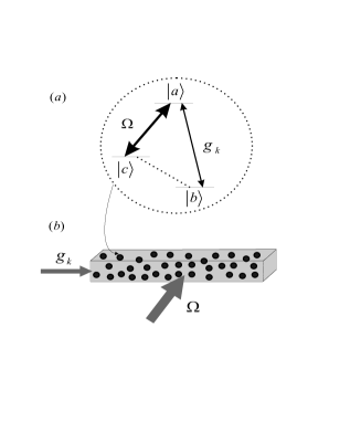
FIG. 1.: Configuration of the quantum memory with $\Lambda$-type atoms. (a) attached on lattice sites of crystal. (b) resonantly coupled to a control classical field and a quantized probe field.

Generalizing the definition of the excitation operators of single optical mode in the Ref. [19], we introduce a class of collective excitation operators of optical multi-mode

$$A_{k}=\frac{1}{\sqrt{N}}\sum_{{\bf j}=1}^{N}e^{-i{\bf k}\cdot{\bf r}_{j}}\sigma_{ba}^{{\bf j}}$$ (3)

with respect to the transition from $|b\rangle$ to $|a\rangle$ for each wave vector ${\bf k}$. Correspondingly, the collective virtual transition from $|b\rangle$ to $|c\rangle$ can be described by another class of collective operators

$$C_{k}=\frac{1}{\sqrt{N}}\sum_{{\bf j}=1}^{N}e^{-i{\bf Q(k)}\cdot{\bf r}_{j}}\sigma_{bc}^{{\bf j}},$$ (4)

where ${\bf Q(k)}={\bf k}-{\bf q}$ means the momentum conservation in the virtual process of collective transition from $|b\rangle$ to $|c\rangle$. These collective operators create the general collective excitations

$\displaystyle|{\bf m},{\bf n}\rangle=\mathop{\displaystyle\prod}_{k}(\frac{1}{\sqrt{m_{k}!n_{k}!}}A_{k}^{\dagger m_{k}}C_{k}^{\dagger n_{k}})|{\bf b}\rangle$

defined for the set of multi-indices

$\displaystyle{\bf m=(}m_{1,}m_{2,}...),{\bf n=(}n_{1,}n_{2,}...),$

and the collective ground state

$\displaystyle|{\bf b}\rangle=|b,b,\cdots,b\rangle$

with all $N$ atoms staying in the same single particle ground state $|b\rangle$. For example, the single particle excitations $|1_{a}\rangle_{k}\equiv A_{k}^{\dagger}|{\bf b}\rangle$ and $|1_{c}\rangle_{k}\equiv C_{k}^{\dagger}|{\bf b}\rangle$. These excitations are easy to understand. Indeed, it is obvious that, from the ground state $|{\bf b}\rangle$, the first order perturbation of the interaction creates the so-called one exciton quasi-spin wave state

$$|1_{a}\rangle_{k} = \frac{1}{\sqrt{N}}\sum_{{\bf j}=1}^{N}e^{i{\bf k}\cdot{\bf r}_{j}}|b,b,\cdots,\stackrel{{\scriptstyle{\bf j-}th}}{{\overbrace{a}}},\cdots,b\rangle,$$ (5)

$$|1_{c}\rangle_{k} = \frac{1}{\sqrt{N}}\sum_{j=1}^{N}e^{i{\bf Q(k)}\cdot{\bf r}_{j}}|b,b,\cdots,\stackrel{{\scriptstyle{\bf j-}th}}{{\overbrace{c}}},\cdots,b\rangle.$$ (6)

Physically, in the large $N$ limit under the low excitation condition, that is, there are only a few atoms occupying the states $|a\rangle$ or $|c\rangle$ [21] and the population of state $|b\rangle$ is approximately $N\rightarrow\infty$, the above two classes of quasi-spin wave excitations behave as two classes of bosons since they have the following bosonic commutation relations

$$[A_{k},A_{k^{\prime}}^{\dagger}] = \delta_{k,k^{\prime}},$$ (7)

$$[C_{k},C_{k^{\prime}}^{\dagger}] = \delta_{k,k^{\prime}},$$ (8)

$$[A_{k},C_{k^{\prime}}^{\dagger}] = 0.$$ (9)

To prove the above basic commutation relations, we first calculate

$$[A_{k},A_{k^{\prime}}^{\dagger}] = =\frac{1}{N}\sum_{{\bf j}=1}^{N}e^{-i({\bf k}^{\prime}-{\bf k)}\cdot{\bf r}_{j}}(\sigma_{bb}^{{\bf j}}-\sigma_{aa}^{{\bf j}})$$

$$\simeq \frac{1}{N}\sum_{{\bf j}=1}^{N}e^{-i({\bf k}^{\prime}-{\bf k)}\cdot{\bf r}_{j}}.$$

Here we have considered that

$$\sum_{{\bf j}=1}^{N}e^{-i({\bf k}^{\prime}-{\bf k)}\cdot{\bf r}_{j}}(\sigma_{bb}^{{\bf j}}-\sigma_{aa}^{{\bf j}})\approx\sum_{{\bf j}=1}^{N}e^{-i({\bf k}^{\prime}-{\bf k)}\cdot{\bf r}_{j}}\sigma_{bb}^{{\bf j}}$$ (10)

while

$$\sum_{{\bf j}=1}^{N}e^{-i({\bf k}^{\prime}-{\bf k)}\cdot{\bf r}_{j}}\sigma_{aa}^{{\bf j}}\approx 0$$ (11)

in the case of low excitation. For a crystal with regular lattice structure, according to the theory of solid state, we should have

$$\frac{1}{N}\sum_{{\bf j}=1}^{N}e^{-i({\bf k}^{\prime}-{\bf k)}\cdot{\bf r}_{j}}=\delta_{{\bf k,k}^{\prime}}.$$ (12)

In fact, this result can be extended to the case of generic medium. For a medium with a scale $L$ much larger than $\frac{2\pi}{\left|{\bf k}\right|},\frac{2\pi}{\left|{\bf k}^{\prime}\right|}$ (this is valid for normal case), the summation over ${\bf r}_{j}$ can be replaced by integral and it follows that

$$\frac{1}{N}\sum_{{\bf j}=1}^{N}e^{-i({\bf k}^{\prime}-{\bf k)}\cdot{\bf r}_{j}}=\frac{1}{V_{me}}\int_{V_{me}}e^{-i({\bf k}^{\prime}-{\bf k)}\cdot{\bf r}}d^{3}{\bf r}\simeq\delta_{{\bf k,k}^{\prime}}$$ (13)

since the medium volume $V_{me}\rightarrow\infty$. The other commutation relations can be proved in a similar way.

III Parallelism Quantum Memory with Hidden Symmetry

As argued above physically the operators $A_{k}$ and $C_{k}$ depict the collective-excitation processes of bosonic type. The importance of  these operators lies in that they define an invariant subspace

$$V_{C}:span\{|{\bf m},{\bf n}\rangle|{\bf m=(}m_{1,}m_{2}...),{\bf n=(}n_{1,}n_{2,}...)\}$$ (14)

for the interaction Hamiltonian (2). This means that driven by this Hamiltonian, any collective state from $V_{C}$ involves to a new collective state still in $V_{C}$. Thus we can use the collective excitations as basic blocks to describe the quantum dynamic process with a hidden symmetry.

Let us introduce the following additional collective operators concerning the transition from $|c\rangle$ to $|a\rangle$

$$T_{-}=\sum_{{\bf j}=1}^{N}e^{-i{\bf q}\cdot{\bf r}_{j}}\sigma_{ca}^{{\bf j}},T_{+}=(T_{-})^{\dagger}$$ (15)

which is resonantly driven by a classic light. Together with the third collective operator

$\displaystyle T_{3}=\sum_{{\bf j}=1}^{N}(\sigma_{aa}^{{\bf j}}-\sigma_{cc}^{{\bf j}})/2,$

they generate $SU(2)$ algebra globally. The commutation relations  between $SU(2)$ and the collective operators $A_{k}$ and $C_{k}$ are easy to calculate. The non-vanishing commutators are as follows:

$$[T_{-},C_{k}] = -A_{k},[T_{+},A_{k}]=-C_{k},$$ (16)

$$\left[T_{+},C_{k}^{\dagger}\right] = A_{k}^{\dagger},\left[T_{-},A_{k}^{\dagger}\right]=C_{k}^{\dagger}.$$ (17)

The above close commutation relations and the expression of the interaction Hamiltonian in terms of these excitation operators:

$$H=\sum_{k}g_{k}\sqrt{N}a_{k}A_{k}^{\dagger}+\Omega T_{+}+h.c.$$ (18)

show that there is a dynamic ”group” (algebra) $G_{d}$ for the light excited system, which is generated by $A_{k}$, $C_{k}$, $A_{k}^{\dagger}$, $C_{k}^{\dagger}$ ($k=1,2,...$), $T_{\pm}$ and $T_{3}$. Using $\Xi$ to denote the Heisenberg-Weyl algebra generated by $A_{k}$, $C_{k}$, $A_{k}^{\dagger}$ and $C_{k}^{\dagger}$ ($k=1,2,...$), we observe that the dynamic ”group” $G_{d}=SU(2)\stackrel{{\scriptstyle-}}{{\otimes}}$ $\Xi$ is a semi-direct product of $SU(2)$ and $\Xi$ because

$$[SU(2),\Xi]\subset\Xi.$$ (19)

Actually the above dynamic symmetry of $G_{d}$ is a straightforward generalization of the symmetry of the single quantized optical mode. With this  symmetry the Hamiltonian $H$ can be diagonalized in an elegant way by means of the spectrum generating algebra method [25] .

To this end we calculate the commutators of $H$ with the generators of $G_{d}$ and light field operators respectively:

$$[C_{k},H] = \Omega A_{k},[A_{k},H]=\Omega C_{k},$$ (20)

$$[a_{k},H] = g_{k}\sqrt{N}A_{k}.$$ (21)

It follows that the dark-state polariton operators

$$D_{k}=a_{k}\cos\theta_{k}-C_{k}\sin\theta_{k}$$ (22)

commute with the Hamiltonian $H$ for the $\theta_{k}$ satisfying

$$\tan\theta_{k}=\frac{g_{k}\sqrt{N}}{\Omega}.$$ (23)

It is obvious that the dark-state polariton operators satisfy the bosonic commutation relations and define new dressed excitations mixing the electromagnetic field and collective excitations of quasi spin wave. Especially these new excitations are stable since

$$[D_{k},H]=0.$$ (24)

For the construction of the complete collective space dressed by the quantized light fields, another ingredient is the bright-state polariton operators

$$B_{k}=a_{k}\sin\theta_{k}+C_{k}\cos\theta_{k}$$ (25)

satisfying

$\displaystyle[D_{k},B_{k}]=0.$

It also extrapolates from the light field of $a_{k}$ to the exciton of $C_{k}$ when one adiabatically changes $\theta_{k}$ from $\frac{\pi}{2}$ to zero. Evidently, the product state $|{\bf 0}\rangle=|{\bf b}\rangle\otimes|0\rangle_{l}$ is an eigen-state of $H$ with zero eigen-value where $|0\rangle_{l}$ is the vacuum of the electromagnetic field. So we can construct a degenerate class of zero eigen-value-states or dark states

$$|d({\bf n)}\rangle\equiv|d({\bf n,}t{\bf)}\rangle=\mathop{\displaystyle\prod}_{k}\frac{1}{\sqrt{n_{k}!}}D_{k}^{\dagger n_{k}}|{\bf 0}\rangle,$$ (26)

where the adiabatic time-dependence originates from the change of Rabi-frequency $\Omega$ for the artificially-controlled classical field. The fact that dark states are cancelled by $H$ means they can trap the electromagnetic radiation from the excited states. Physically this is due to quantum interference cancelling.

With the help of the above hidden symmetry we can also construct the energy spectra with non-zero eigenvalues by using the bright-state polariton operators. We start from the derived commutation relations from the above equation (21)

$$[H,B_{k}^{\dagger}] = \Theta_{k}A_{k}^{\dagger},$$ (27)

$$[H,A_{k}^{\dagger}] = \Theta_{k}B_{k}^{\dagger},$$ (28)

where

$$\Theta_{k}=\sqrt{g_{k}^{2}N+\Omega^{2}}.$$ (29)

This prompts us to consider the two commuting quasi-boson operators

$$Q_{k\pm}=\frac{1}{\sqrt{2}}(A_{k}\pm B_{k}).$$ (30)

As we have the commutation relations

$$[H,Q_{k\pm}^{\dagger}]=\pm\Theta_{k}Q_{k\pm}^{\dagger},$$ (31)

the operators $Q_{k\pm}$ can serve as ladder operators to generate the spectra of $H.$ In fact they produce the dressed states of the multi-mode exciton system

$$|e({\bf m,s,n)}\rangle=\mathop{\displaystyle\prod}_{k}\frac{1}{\sqrt{m_{k}!s_{k}!}}Q_{k+}^{\dagger m_{k}}Q_{k-}^{\dagger s_{k}}|d({\bf n)}\rangle$$ (32)

as the eigen-states of $H$ with the eigen-values

$$E({\bf m,s)}=\sum_{k}(m_{k}-s_{k})\Theta_{k},$$ (33)

of infinite degeneracy degrees.

Now we consider the relation between the degeneracy of spectrum and the hidden symmetry. We notice that the infinite degeneracy of $|e({\bf 0,0,n)}\rangle=|d({\bf n)}\rangle$ results from the generalized translation symmetry described by

$$T_{k} = \exp(\alpha_{k}D_{k}^{\dagger}-\alpha_{k}^{\ast}D_{k})$$ (34)

$$= {\cal D}_{a_{k}}(\alpha_{k}\cos\theta_{k}){\cal D}_{C_{k}}(-\alpha_{k}\sin\theta_{k}),$$ (35)

where

$\displaystyle{\cal D}_{a}(\alpha)=\exp(\alpha a^{\dagger}-\alpha^{\ast}a)$

is the usual coherent state generator. In fact, for the original Hamiltonian (2), the unitary transformation ${\cal D}_{a_{k}}(\alpha_{k}\cos\theta_{k})$ changes the term $g_{k}\sqrt{N}a_{k}A_{k}^{\dagger}$ by $g_{k}\sqrt{N}A_{k}^{\dagger}\alpha_{k}\cos\theta_{k}$ while ${\cal D}_{C_{k}}(-\alpha_{k}\sin\theta_{k})$ changes the terms $\Omega T_{+}$ by $-g_{k}\sqrt{N}A_{k}^{\dagger}\alpha_{k}\sin\theta_{k}$ since

$\displaystyle{\cal D}_{a_{k}}^{-1}(\alpha_{k}\cos\theta_{k})a_{k}{\cal D}_{a_{k}}(\alpha_{k}\cos\theta_{k})=a_{k}+\alpha_{k}\cos\theta_{k},$

$\displaystyle{\cal D}_{C_{k}}^{-1}(-\alpha_{k}\sin\theta_{k})T_{+}{\cal D}_{C_{k}}(-\alpha_{k}\sin\theta_{k})=T_{+}-A_{k}^{\dagger}\alpha_{k}\sin\theta_{k}.$

These two changes cancel each other. Besides this degeneracy for different ${\bf n}$, due to the relation

$$[H,Q_{k+}^{\dagger}Q_{k-}^{\dagger}]=0,$$ (36)

there are a large additional class of dark states of zero-eigen-value. They can be constructed by acting $Q_{k+}^{\dagger}Q_{k-}^{\dagger}$ repeatedly on $|d({\bf n)}\rangle$.

The above arguments suggest that, compared with the single mode exciton system the dressed multi-mode exciton system generated by $A_{k}^{\dagger},B_{k}^{\dagger}$ and $a_{k}^{\dagger}$ can serve as a quantum memory with more advantages. It is very interesting that all the parameters $\theta_{k}$ for different modes of $k$ can be well controlled to change from zero to infinity by a unique extremely slow adiabatic parameter $\Omega=\Omega(t)$ varying from a very large value to zero. As usual, the quantum information of photons is described by the superposition state

$$|L(0)\rangle=\sum_{{\bf n}}c_{{\bf n}}\,|{\bf n}\rangle_{l}\equiv\sum_{{\bf n}}c_{{\bf n}}\mathop{\displaystyle\prod}_{k}\frac{1}{\sqrt{n_{k}!}}a_{k}^{\dagger n_{k}}|0\rangle_{l}$$ (37)

where $|{\bf n}\rangle_{l}$ is a multi-mode Fock state for the light field. In the case $\Omega(0)\rightarrow\infty$, whatever the values of the parameters are we have $\sin\theta_{k}=0$ so $|d({\bf n,0)}\rangle=|{\bf b}\rangle\otimes|{\bf n}\rangle_{l}$ and the initial state of total system can be expressed as a superposition of the adiabatic dark states $|d({\bf n,0)}\rangle$ at time $t=0:$

$$|S(0)\rangle=|{\bf b}\rangle\otimes\sum_{{\bf n}}c_{{\bf n}}\,|{\bf n}\rangle_{l}=\sum_{{\bf n}}c_{{\bf n}}\,|d({\bf n,0)}\rangle$$ (38)

By adiabatically changing $\Omega$ to zero at time $T$, each component in the above superposition varies in this way:

$\displaystyle|d({\bf n,0)}\rangle\rightarrow|d({\bf n,T)}\rangle=|{\bf n}\rangle_{C}\otimes|0\rangle_{l}.$

Thus one extrapolates $|S(0)\rangle$ to a pure multi-exciton state

$$|S(T)\rangle=\sum_{{\bf n}}c_{{\bf n}}\,|{\bf n}\rangle_{C}\otimes|0\rangle_{l},$$ (39)

where

$$|{\bf n}\rangle_{C}=\mathop{\displaystyle\prod}_{k}\frac{1}{\sqrt{n_{k}!}}C_{k}^{\dagger n_{k}}|{\bf b}\rangle$$ (40)

is the multi mode exciton state describing the collective excitation.

It is worth pointing out that, the above observation based on the dynamic symmetry does not depend on the adiabaticallity of manipulation on the external parameters at all. In our example, because the dark states don’t contain any atomic excited state $|a\rangle$, the spontaneous emission is then forbidden even for a non-adiabatic manipulation. By the way we also point out that the quantum parallelism of the multi-mode exciton quantum memory gives rise to a very convenient encoding process. For a decimal system number $n$ there is a unique binary representation:

$$n=\sum_{i=0}^{L-1}n_{i}2^{i}$$ (41)

where $n_{i}=0,1$. Then we can encode it in a special multi-mode Fock state

$$|{\bf n}\rangle_{l}=|n_{0,}n_{1,}n_{2,}...,n_{L-1}\rangle$$ (42)

of light field. The multi-mode Fock state $|{\bf n}\rangle_{l}$ can be represented by an array of the many-photon qubits, with at most one photon in each photon qubit. It is easy to prepare such photon state in flying (photon) qubit firstly and then store the decimal system number $n$ in the above multi-mode exciton quantum memory as a single component many-exciton state $|{\bf n}\rangle_{C}$.

IV Transient Dynamics of Light Propagation

In the previous sections, making full use of the hidden symmetry, we not only construct two classes of dark states and their generated spectra of non-zero eigenvalues, but also demonstrate that coherent optical information of multi-qubit can be stored in a medium with collective effect in EIT. The storing and reading-out processes are controlled by stimulated photon transfer between the classical and quantized light field. In this section we will consider the transient dynamic process for the interaction between light fields and the EIT medium. Some exotic natures of light propagation in such a medium will be investigated with the help of the dynamic symmetry analysis.

The evolution of the Heisenberg operators corresponding to the optical field and the collective excitations can be described as

$$\stackrel{{\scriptstyle.}}{{a}}_{k} = -i\sqrt{N}g_{k}A_{k},$$ (43)

$$\stackrel{{\scriptstyle.}}{{A}}_{k} = -i\sqrt{N}g_{k}a_{k}-i\Omega C_{k},$$ (44)

$$\stackrel{{\scriptstyle.}}{{C}}_{k} = -i\Omega A_{k}$$ (45)

for each light mode ${\bf k}$. The above motion equations of $a_{k}$, $A_{k}$ and $C_{k}$ with respect to a given optical mode ${\bf k}$ are coupled together, but there is no coupling of mode ${\bf k}$ operators to those of different optical mode ${\bf k}^{\prime}$. Due to the semi-direct product property of the dynamic group $G=SU(2)\stackrel{{\scriptstyle-}}{{\otimes}}\Xi\otimes\Gamma,$ the generators $T_{+}$, $T_{-}$, and $T_{3}$ of $SU(2)$ algebra do not occur in the above system of Heisenberg equations. Here $\Gamma$ is the Heisenberg-Weyl group generated by the creation and annihilation operators $a_{k}^{\dagger}$ and $a_{k}$. It leads to the evolution equations of the bright- and dark- state polariton operators

$$\stackrel{{\scriptstyle.}}{{A}}_{k} = -i\sqrt{g_{k}^{2}N+\Omega^{2}}B_{k},$$ (46)

$$\stackrel{{\scriptstyle.}}{{B}}_{k} = -i\sqrt{g_{k}^{2}N+\Omega^{2}}A_{k},$$ (47)

$$\stackrel{{\scriptstyle.}}{{D}}_{k} = 0$$ (48)

in a straightforward way. The above equations manifest the basic features of the dark states: decoupled from other states and stable in the time evolution.

With the initial conditions determined by those for $C_{k}$ and $a_{k}$, the exact solutions of $B_{k}$ and $D_{k}$ are obtained as follows:

$$D_{k}(t)=D_{k}(0)=a_{k}(0)\cos\theta_{k}-C_{k}(0)\sin\theta_{k},$$ (49)

$$B_{k}(t)={\bf O}_{1}e^{-it\Theta_{k}}+{\bf O}_{2}e^{it\Theta_{k}}],$$ (50)

$${\bf O}_{1} = \frac{1}{2}(B_{k}(0)-A_{k}(0))$$

$${\bf O}_{2} = \frac{1}{2}(B_{k}(0)+A_{k}(0))$$

where $a_{k}(0),$ $A_{k}(0),$ $B_{k}(0)$ and $C_{k}(0)$ are the initial Heisenberg operators, and $\Theta_{k}=\sqrt{g_{k}^{2}N+\Omega^{2}}$ is the light field dressed Rabi frequency that measures the effective coupling of excitonic states to the external field.

The dark-state polariton operator $D_{k}(t)$ is indeed a time-independent constant. That is, in the Heisenberg picture, the operator $D_{k}(t)$ always retains the initial ${\bf k-}$mode dark-state polariton operator $D_{k}(0)$ for each ${\bf k}$ and the atomic system always keeps being an EIT medium. Here for simplicity we assume that the quantized light field propagates along the $x-$axis. Then, the positive frequency part of the quantized light field

$$E^{+}(x,t)=\sum_{k}\sqrt{\frac{\hbar ck}{2\epsilon V}}a_{k}(t)e^{ikx-ikct}$$ (51)

can be expressed explicitly in terms of the mode operators of quantized light field

$$a_{k}(t) = D_{k}(t)\cos\theta_{k}+B_{k}(t)\sin\theta_{k}$$ (52)

$$= [a_{k}(0)\cos\theta_{k}-C_{k}(0)\sin\theta_{k}]\cos\theta_{k}$$ (54)

$$-({\bf O}_{1}e^{-it\Theta_{k}}+{\bf O}_{2}e^{it\Theta_{k}})\sin\theta_{k},$$

which results from the expressions of bright- and dark- state polariton operators given above.

With the above simple solution we can straightforwardly investigate how the quantized light propagates in the EIT medium. We assume that the collective state of the medium is initially in the ground state $|{\bf b\rangle}$ and the initial state of the light field is a wave packet. The electromagnetic field quantized, the wave packet of light can be depicted by the direct product of many coherent states, or the multi-mode coherent state

$$|{\bf\alpha}\rangle=\prod_{k}\otimes|\alpha_{k}\rangle,$$ (55)

where $\alpha_{k}=\exp[-f^{2}(k-k_{0})^{2}]$ (up to a normalized factor) since the probe light is a Gaussian wave packet in frequency domain. This is because the expectation value of the free quantized electromagnetic field operator

$\displaystyle E^{+}(x,t)=\sum_{k}\sqrt{\frac{\hbar ck}{2\epsilon V}}a_{k}(t)e^{ikx-ikct}$

resembles a classical wave packet as the superposition of infinite components of different frequencies. In interaction with EIT medium, the mean of $a_{k}(t)$ over the initial state $|\psi(0)\rangle=|{\bf b\rangle}\otimes|{\bf\alpha}\rangle$ is

$$\langle a_{k}(t)\rangle = \langle a_{k}(0)\rangle\cos^{2}\theta_{k}+$$ (57)

$$\sin\theta_{k}(\langle{\bf O}_{2}\rangle e^{-it\Theta_{k}}+\langle{\bf O}_{1}\rangle e^{it\Theta_{k}})$$

$$= \langle a_{k}(0)\rangle(\cos^{2}\theta_{k}+\sin^{2}\theta_{k}\cos\Theta_{k}t),$$ (58)

where we have used

$$\langle A_{k}(0)\rangle = \langle C_{k}(0)\rangle=0,$$

$$\langle B_{k}(0)\rangle = \langle a_{k}(0)\rangle\sin\theta_{k}.$$

So the mean of $E^{+}(x,t)$ is decomposed into three parts:

$$\langle E^{+}(x,t)\rangle = \sum_{k}\sqrt{\frac{\hbar ck}{2\epsilon V}}\langle a_{k}(0)\rangle\times$$ (60)

$$(\cos^{2}\theta_{k}+\sin^{2}\theta_{k}\cos\Theta_{k}t)e^{i(kx-kct)}$$

$$= E_{0}^{+}(x,t)+E_{+}^{+}(x,t)+E_{-}^{+}(x,t)$$ (61)

where

$$E_{+}^{+}(x,t) = \sum_{k}\sqrt{\frac{\hbar ck}{2\epsilon V}}\langle a_{k}(0)\rangle\sin^{2}\theta_{k}e^{i[k(x-ct)-\Theta_{k}t]},$$ (62)

$$E_{0}^{+}(x,t) = \sum_{k}2\sqrt{\frac{\hbar ck}{2\epsilon V}}\langle a_{k}(0)\rangle\cos^{2}\theta_{k}e^{ik(x-ct)},$$ (63)

$$E_{-}^{+}(x,t) = \sum_{k}\sqrt{\frac{\hbar ck}{2\epsilon V}}\langle a_{k}(0)\rangle\sin^{2}\theta_{k}e^{i[k(x-ct)+\Theta_{k}t]}.$$ (64)

It should be noticed that the light field dressed Rabi frequency $\Theta_{k}$ modifies the dispersion relations of light propagation in the exciton medium.

The three parts in the above decomposition of $\langle E^{+}(x,t)\rangle$ can be understood as three wave packets spreading in the coordinate space. We can see this point by considering the initial quantized light field in the frequency domain as a Gaussian wave packet with the center frequency $\omega_{0}$ ($=k_{0}c=\omega_{ab}$). For the first wave packet $E_{+}^{+}(x,t)$, its position center is determined by maximizing the wave-vector-dependent phase:

$$\frac{\partial}{\partial k}(kct+\Theta_{k}t-kx)|_{k_{0}}=0.$$ (65)

This determines the group velocity of the wave packet $E_{+}^{+}(x,t)$ as

$$V_{g_{+}}=\frac{\partial x}{\partial t}|_{k_{0}}=c+\frac{\partial\Theta_{k}}{\partial k}|_{k_{0}}.$$ (66)

The term on the r.h.s. simply leads to a modification of the group velocity

$$V_{g_{+}}=c(1+\frac{\Omega}{2k_{0}c}\frac{n}{\sqrt{1+n}}),$$ (67)

where $n=\frac{g_{k_{0}}^{2}N}{\Omega^{2}}$. This is one of the central results of this paper. It is evident that the first wave packet $E_{+}^{+}(x,t)$ represents the ”super-luminal” light propagation with the group velocity larger than the light speed $c$. It is also emphasized that the ”super-luminal” light propagation can be understood according to the classical theory of wave propagation in an anomalous dispersion medium. It is the interference between different frequency components that results in this rather counterintuitive effect. In this sense, we think that the ”super-luminal” light pulse propagation observed in experiments is not too odd and there is no direct connection between this phenomenon and the causality in relativity.

It is not surprising to see the usual group velocity $V_{g_{0}}=c$ for the second wave packet $E_{0}^{+}(x,t)$. But for the third wave packet $E_{-}^{+}(x,t)$ we find the sub-luminal group velocity similarly:

$$V_{g_{-}} = c-\frac{\partial\Theta_{k}}{\partial k}|_{k_{0}}$$ (68)

$$= c(1-\frac{\Omega}{2k_{0}c}\frac{n}{\sqrt{1+n}}).$$ (69)

This sub-luminal group velocity phenomenon is expected to find applications in quantum information processing. In fact, it is common sense to believe that the system stopping and slowing light could be used to store quantum information of photon qubits and in the storage time quantum information processing may be possible if we can sufficiently reduce the dissipative loss during the ”reading” and ”writing” operations.

We can also analytically integrate out $E_{0}^{+}(x,t)$, $E_{+}^{+}(x,t)$ and $E_{-}^{+}(x,t)$ and obtain an explicit depiction of the propagating wave packet. Since $g_{k}=-\wp\sqrt{\frac{kc}{2\hbar\epsilon V}}$, it is convenient to write $g_{k}^{2}N$ as $G^{2}k$ with $G=\wp\sqrt{\frac{cN}{2\hbar\epsilon V}}$. Replacing the summation over $k$ by integral and using $\langle a_{k}(0)\rangle=\alpha_{k}$, we obtain the normal part

$$E_{0}^{(+)}(x,t) = \frac{1}{2\pi}\int 2L_{m}\sqrt{\frac{ck}{2\epsilon V}}\frac{\Omega^{2}}{\Omega^{2}+G^{2}k}$$ (71)

$$\times e^{-f^{2}(k-k_{0})^{2}}e^{ik(x-ct)}dk,$$

and the super-luminal and sub-luminal (or negative) parts

$$E_{\pm}^{(+)}(x,t) = \frac{1}{2\pi}\int L_{me}\sqrt{\frac{ck}{2\epsilon V}}\frac{G^{2}k}{\Omega^{2}+G^{2}k}$$ (73)

$$\times e^{-f^{2}(k-k_{0})^{2}}e^{ikx-it(kc\pm\Theta_{k})}dk,$$

where $L_{me}$ is the scale of integration along the propagation direction ($x$-axis) of the probe light. We then expand the terms $\sqrt{k},$ $\frac{\Omega^{2}}{\Omega^{2}+G^{2}k},$ $\frac{G^{2}k}{\Omega^{2}+G^{2}k}$ and $\Theta_{k}$ around the central value $k_{0}$ of the wave vector of the input probe light. We can neglect the higher-order terms of $\Delta$ $=k-k_{0}$ since $k$ is very close to $k_{0}$. Then, with the defined parameters $A=G^{2}/\Omega^{2}$, $\Omega_{0}=\Omega\sqrt{1+Ak_{0}}$, the approximate expressions of field components are obtained analytically as

$$E_{\pm}^{(+)}(x,t) \approx \frac{Ak_{0}\sqrt{\pi k_{0}}}{2f^{3}(1+Ak_{0})}\{2f^{2}+iD_{0}[x-(c\pm E_{0})t]\}$$ (75)

$$\times\exp[-\frac{1}{4f^{2}}[x-(c\pm E_{0})t]^{2}]e^{ik_{0}(x-c_{\pm}t)}$$

and

$$E_{0}^{(+)}(x,t) \approx \frac{\sqrt{\pi k_{0}}}{2f^{3}(1+Ak_{0})}[2f^{2}+iF_{0}(x-ct)]$$ (77)

$$\times\exp[-\frac{1}{4f^{2}}(x-ct)^{2}]e^{ik_{0}(x-ct)},$$

where $c_{\pm}=c\pm\frac{\Omega_{0}}{k_{0}}$ and

$$D_{0} = \frac{3+Ak_{0}}{2k_{0}(1+Ak_{0})},$$

$$E_{0} = \frac{\Omega_{0}A}{2(1+Ak_{0})},$$

$$F_{0} = \frac{1-Ak_{0}}{2k_{0}(1+Ak_{0})}.$$

The above analytic result proves again the coexistence phenomena of both the super-luminal and sub-luminal (or negative) group velocities. From the Eqs. (75,77), it’s obvious that the group velocity of the part $E_{0}^{(+)}(x,t)$ is $V_{g_{0}}=c,$ and the group velocity of wave packet $E_{\pm}^{+}(x,t)$ is

$$V_{g_{\pm}}=c\pm E_{0}=c(1\pm\frac{\Omega}{2k_{0}c}\frac{n}{\sqrt{1+n}})$$ (78)

which is the same as the Eqs. (67) and (69).

Through the above theoretical analysis based on dynamic algebraic method, several interesting properties of the light pulse propagation in an EIT medium are observed. The central result is the possibility of coexistence of ”sub-luminal” and ”super-luminal” group velocity phenomena, occurring as a triple split of wave packet when spreading in such an EIT medium. We also observe that if we inject coherent light into the EIT medium for a certain time, there may appear three light pulses. One of these three light pulses still propagates at the velocity $c$, but the other two have ”super-luminal” and ”sub-luminal” group velocities respectively. The ”sub-luminal” group velocity might even have negative value in some case. This result is different from that of stable process in which only one single group velocity appears. This is because we here only consider the transient phenomenon or property. It is also remarked that both ”super-luminal” and “sub-luminal” (even or negative) group velocities are natural properties of light [4] and could be realized experimentally.

V Numerical Simulation of Wave Packet Split

In this section we numerically simulate the dynamic process of the light pulse propagating in the above described EIT medium. According to the Eqs. (75,77), we calculate the shape evolutions of the wave packets of the three parts of the light field, respectively. Let $\lambda_{0}=\frac{2\pi}{k_{0}}=\frac{2\pi c}{\omega_{0}}$ be the central wavelength of the initial wave packet of the light pulse. To simulate the light pulse propagating in the EIT medium numerically we distinguish the following two situations: (I) the spatial width$\ d$ of light pulse is less than $\lambda_{0}$; (II) $d$ contains a few $\lambda_{0}$’s. In the second situation several oscillations will be clearly observed in a light pulse with a few frequency components. Let $E_{i}(x,t)=E_{i}^{+}(x,t)+$ $E_{i}^{-}(x,t)$, for $i=0,+,-$. For situation (I) that the spatial width$\ d$ of light pulse is less than its central wavelength ($d\approx 0.3\lambda_{0})$, three 3-dimension curves of $E_{0}(x,t)$, $E_{+}(x,t)$ and $E_{-}(x,t)$ are plotted as in Fig. 2. It is observed from Fig. 2 the three parts $E_{0}(x,t)$, $E_{+}(x,t)$ and $E_{-}(x,t)$ of light field indeed have different group velocities. It’s noted that in order to satisfy the near-resonance condition, the experimental probe light pluse contains large numbers of wavelengths much more than that given above where it’s convenient to see the pulse splitting.

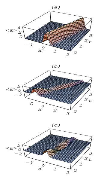
FIG. 2.: Wave packet split of light pulse in the case that the spatial width of light pulse is less than its central wavelength $d\approx 0.3\lambda_{0})$: (a): the normal part with group velocity $c$. (b): the super-luminal part with group velocity being about $1.75c$. (c) the sub-luminal part with group velocity being about$0.25c$.

Fig. 3 is drawn  for the situation (II) that the spatial width$\ d$ of light pulse is large than its central wavelength ( $d\approx 4\lambda_{0})$. In both of the situations it is observed that the group velocity ($v\simeq 1.75c)$ of $E_{+}(x,t)$ is larger than that of $E_{0}(x,t),$ but the group velocity ($v\simeq 0.25c)$ of $E_{-}(x,t)$ is less than that of $E_{0}(x,t).$The only difference between these two situations is the details of the oscillations of the caves.

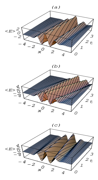
FIG. 3.: Wave packet split of light pulse in the case that the spatial width of light pulse is large than its central wavelength $d\approx 4\lambda_{0})$: (a): the normal part with group velocity $c$. (b):the super-luminal part with group velocity $v=0.25c$. (c): a sub-luminal part with group velocity $v=1.75c$. The other parameters is as the same as that in Fig. 2.

When the system parameters are changed so that

$$\frac{\Omega}{2k_{0}c}\frac{n}{\sqrt{1+n}}>1.$$ (79)

a seem-to-be exotic phenomenon of light pulse propagation is illustrated in Fig. 4. Here, while two parts of the splitting wave packet (Fig.4a-4b) possess normal group velocity $c$ and ”super-luminal” group velocity $(v\simeq 2.36c)$ respectively, the third part propagates at a negative group velocity $(v\simeq-0.36c).$

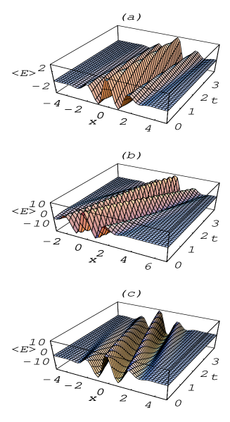
FIG. 4.: Propagation of light pulse with a part possessing a negative group velocity $(\simeq-0.36c)$. Here, the spatial width of light pulse is large than its central wavelength $d\approx 4\lambda_{0})$: (a): the normal part with group velocity $c$. (b) the super-luminal part with group velocity $v\simeq-0.36c$. (c) the part propagating with a negative group velocity $(v\simeq 2.36c).$

In fact the amplitude of these field components depends on the system parameters. It is easily seen from Eq. (63) that the intensity of $E_{+}(x,t)$ is equal to that of $E_{-}(x,t)$, but is not equal to that of $E_{0}(x,t)$. The ratio of the amplitude of $E_{\pm}(x,t)$ to that of $E_{0}(x,t)$ is approximately

$$\frac{\sin^{2}\theta_{k_{0}}}{2\cos^{2}\theta_{k_{0}}}=\frac{g_{k_{0}}^{2}N}{2\Omega^{2}}=\frac{n}{2}.$$ (80)

When the ratio $\frac{n}{2}$ is very small ($\ll 1$), most part of the light pulse will propagate in the EIT medium at the group velocity $c$. If the ratio $\frac{n}{2}$ is very large ($\gg 1$), then most part of the light pulse propagates at ”super-luminal” or sub-luminal (even negative) group velocity. To see the dynamic details clearly we also plot the caves of the spatial wave packets for different fixed instances in Fig. 5.

FIG. 5.: Evolution of three splitting wave packets of light pulse. Here, $d=4\lambda_{0})$ (a) The initial un-split wave packet with the spatial width of light pulse $d\approx 4\lambda_{0})$;(b) [(c)] The shapes of the three splitting wave packets at times $t_{1}\approx 2.3*10^{-13}s$ [ $t_{2}\approx 4.6*10^{-13}s$]. The cases with normal, ”super-luminal” and sub-luminal are depicted respectively by solid line,dot line and dash line. The parameters are the same as that in Fig. 3

Fig. 5 (a-c) shows the time evolution of these three wave-packets at $t=t_{0}(=0),t_{1},t_{2}$ ($0<t_{1}<t_{2}$) according to the Fig. 3. The field components $E_{+}(x,t)$ and $E_{-}(x,t)$) with ”super-luminal” and ”sub-luminal” group velocities change their shapes of wave-packet during the evolution, but the part $E_{0}(x,t)$ always propagates at $c$  with an unchanged shape of wave-packet. Due to the intrinsic quantum coherence the EIT medium does not change the height of each wave-packet. Strictly speaking, $c=c_{0}/n_{0}$ is not the vacuum velocity of light, while $c_{0}$ is,where $n_{0}$ is the index of refraction [22] (here for simplicity, we set $n_{0}=1$ in our numerical simulation in this work). To see the exotic phenomenon with negative group velocity, we take the 2-dimension curves at certain time in Fig. 6 according to the Fig. 4. Here, a inverse-direction ”light propagation” can be seen clearly.

FIG. 6.: Phenomenon with a negative group velocity $(v\simeq-0.36c)$. Here, $d=4\lambda_{0})$: (a) The initial un-split wave packet with the spatial width of light pulse $d\approx 4\lambda_{0})$;(b) [(c)] The shapes of the three splitting wave packets at times $t_{1}\approx 1.3\ast 10^{-13}s$ [ $t_{2}\approx 2.6\ast 10^{-13}s$]. The cases with normal and super-luminal are depicted respectively by solid line and dot line. The dash line describe the a part of the split wave packet propagating with a a negative group velocity $(v\simeq-0.36c).$ The parameters are the same as that in Fig. 4.

We can also calculate the optical intensity in the case, where the initial quantized light field is multi-mode coherent state. We have

$$I(x,t) = \left\langle E^{-}(x,t)E^{+}(x,t)\right\rangle$$ (81)

$$= E_{0}^{+}E_{0}^{-}+E_{+}^{+}E_{+}^{-}+E_{-}^{+}E_{-}^{-}$$ (83)

$$+2\mathop{\rm Re}(E_{0}^{+}E_{+}^{-}+E_{+}^{+}E_{-}^{-}+E_{-}^{+}E_{0}^{-}).$$

From the Eqs. (75) and (77), it’s obvious that $E_{0}^{+}E_{0}^{-}$, $E_{+}^{+}E_{+}^{-}$ and $E_{-}^{+}E_{-}^{-}$ are three approximate Gaussian wave packets respectively and $E_{0}^{+}E_{+}^{-}$ (also $E_{+}^{+}E_{-}^{-}$ and $E_{-}^{+}E_{0}^{-}$) is the interference term. At the initial time $t=0$, $I(x,t)$ is a Gaussian wave packet approximately since the center of each term contributing to $I(x,t)$ is at $x=0$. But after a certain time, the terms $E_{0}^{+}E_{0}^{-}$, $E_{+}^{+}E_{+}^{-}$ and $E_{-}^{+}E_{-}^{-}$ are nearly separated in spatial coordinate and the contribution of interference terms will be close to zero. So in this case the intensity will only contain 3 separated Gaussian wave packets with the ”super-luminal”, ”sub- (even negative) luminal” and normal group velocities respectively.

Finally we consider the quantum fluctuation of the probe quantum field. In the above discussions we assume the quantized light field of each mode to be initially prepared in its coherent state. This is too conceptual a setup for experiment. If the initial state is a number state the expectation of the quantized light field operator vanishes for the representation of photon number conservation. For this reason we need to consider the quantum fluctuation described by the correlation function

$$\left\langle E^{-}(x,t)E^{+}(x,t+\tau)\right\rangle$$ (84)

$$= \sum_{k}\frac{\hbar c\left|k\right|\left\langle n\right\rangle_{k}}{2\epsilon V}e^{ikc\tau}(\cos^{2}\theta_{k}+\sin^{2}\theta_{k}\cos\Theta_{k}t)^{2}.$$ (85)

It will determines the intensity spectra

$$S(x,\omega)\equiv\int_{-\infty}^{\infty}\!\!{\rm d}\tau\,{\rm e}^{-i\omega\tau}\,\left\langle E^{-}(x,t)E^{+}(x,t+\tau)\right\rangle=S(0,\omega).$$ (86)

The one-time correlation is substantially the intensity of the probe light field

$$\left\langle I(x,t)\right\rangle = \left\langle E^{-}(x,t)E^{+}(x,t)\right\rangle$$ (87)

$$= \sum_{k}\frac{\hbar c\left|k\right|\left\langle n\right\rangle_{k}}{2\epsilon V}(\cos^{2}\theta_{k}+\sin^{2}\theta_{k}\cos\Theta_{k}t)^{2}.$$ (88)

As a modulated asymptotic function, this result is illustrated in Fig. 7  for an initial number state with $\left\langle n\right\rangle_{k}$ satisfying a Gaussian wave distribution in frequency domain. It shows the instantaneous process of light propagation to approach a stable state. For very large Rabi coupling constant $\Omega,$ $\theta_{k}\simeq 0,$ $\Theta_{k}=\sqrt{g_{k}^{2}N+\Omega^{2}}\simeq\Omega$ and the  intensity approaches a constant $\left\langle I(x,t)\right\rangle=\sum_{k}\frac{\hbar c\left|k\right|\left\langle n\right\rangle_{k}}{2\epsilon V}.$ On the other hand for a very large medium enhanced coupling of probe light $g_{k}^{2}N$ or $\Omega=0,\theta_{k}\simeq\frac{\pi}{2},$we can analytically show

$$\left\langle I(x,t)\right\rangle = \sum_{k}\frac{\hbar c\left|k\right|\left\langle n\right\rangle_{k}}{2\epsilon V}(\cos g_{k}^{2}Nt)^{2}$$ (89)

$$= \sum_{k}\frac{\hbar c\left|k\right|\left\langle n\right\rangle_{k}}{2\epsilon V}\cos^{2}(\frac{c\wp^{2}N}{2\hbar\epsilon V}kt),$$ (90)

which is asymptotic to a constant with the modulation frequency $\omega_{M}=\frac{c\wp^{2}N}{2\hbar\epsilon V}k$.

FIG. 7.: The intensity evolution of probe light with a modulated asymptotic behavior.

VI Conclusion with Remarks

In conclusion, we have investigated how the quantized light propagates in a three-level $\Lambda-$type EIT medium by directly solving the Heisenberg evolution equation of this light field based on the dynamic group method. For simplicity, the quantized light field is considered as resonantly coupling to the $\Lambda-$type subsystem even though this light field contains a series of light modes and can not be resonant simultaneously. The  physical reason for this consideration is that the light wave packet has a small width in frequency domain. In fact, the quantized light is considered as a quasi-plane wave and propagating in the medium without the boundary effect. It should be noticed that the present treatment is valid only when the EIT medium is prepared in the low density excitation situation.

We wish to emphasize again that it is also owing to the wave nature of light that the coexistence phenomena of both the ”super-luminal” and ”sub-luminal” (or negative) group velocities appears as predicted in this paper. It is very interesting to observe this coexistence phenomena experimentally and explore its potential application in quantum memory and quantum information process. To this end we need more details of physical considerations on the experimental techniques. For instance, we need to compare the size of the sample of the EIT medium and the split distances of three wave packets resulting from the light pulse. In principle due to the different group velocities the evolution of sufficiently-long time will distinguish the wave packets, which might not preserve their shape because of wave packet spreading or the dissipation and decoherence due to the coupling to environment. On the other hand, what we predict are only the transient phenomena.  So it is somehow difficult to observe this coexistence phenomena of both the ”super-luminal” and ”sub-luminal” (or negative) group velocities in a practical experiment.

This work is supported by the NSF of China (CNSF grant No.90203018) and the knowledged Innovation Program (KIP) of the Chinese Academy of Science. It is also founded by the National Fundamental Research Program of China with No 001GB309310. We also sincerely thank Y. Wu, P. Zhang and L. You for the useful discussions with them.

Light Propagation in Exciton System: Analytic Result from Sub-dynamics Mehtod

In general we consider a physical system with a dynamic symmetry characterized by a Lie group $G$. This means that the Hamiltonian of the considered system

$$H=H[G]\equiv H(g_{1},g_{2},...)$$ (A.1)

is a functional of the generators $g_{1},$ $g_{2},...$ of $G$. These generators  can be understood as the basic dynamic variables of the system. Suppose there exists a subgroup $S\subset G$ such that

$$[H,G]\subset S.$$ (A.2)

Let $s_{1},$ $s_{2},...$ be the generators of $S$. Then the system of the Heisenberg equations

$$i\frac{d}{dt}s_{k}=[s_{k},H]\in S$$ (A.3)

about $s_{1},$ $s_{2},...$ are closed to form the so-called sub-dynamics. Through the subset $\{s_{1},s_{2},...\}$ of the complete set of dynamic variables $g_{1},$ $g_{2},...$, the sub-dynamics depict the main features of the considered system.

The excitonic system in this paper serves as a practical example for

$$G=SU(2)\stackrel{{\scriptstyle-}}{{\otimes}}\Xi\otimes\Gamma$$ (A.4)

and $S=$ $\Xi\otimes\Gamma$ where $\Gamma$ is the Heisenber-Weyl group generated by the creation and annihilation operators $a_{k}^{\dagger}$ and $a_{k}$ of light field.

REFERENCES

- [1] Electronic address: suncp@itp.ac.cn
- [2] Internet www site: http://www.itp.ac.cn/~suncp
- [3] L. V. Hau, S. E. Harris, Z. Dutton, and C. H. Behroozi, Nature 397, 594 (1999).
- [4] L. J. Wang, A. Kuzmich, A. Dogariu, Nature, 406, 277 (2000); Y. Shimizu, N. Shiokawa, N. Yamamoto, M. Kozuma, T. Kuga, L. Deng, and E. W. Hagley, Phys. Rev. Lett. 89, 233001 (2002).
- [5] S. E. Harris, Physics Today 50, 36 (1997).
- [6] M. O. Scully, Phys. Rev. Lett. 55, 2802 (1985).
- [7] S. E. Harris, Phys. Rev. Lett. 62, 1033 (1989).
- [8] M. O. Scully, Phys. Rev. Lett. 67, 1855 (1991).
- [9] S. E. Harris et al., Phys. Rev. Lett. 64, 1107 (1990); M. Fleischhauer, M. D. Lukin, A. B. Matsko, and M. O. Scully, Phys. Rev. Lett. 82, 1847 (1999).
- [10] Ö. E. Müstecaplioglu and L. You, Phys. Rev. A 64, 013604 (2001).
- [11] A. V. Turukhin et al., Phys. Rev. Lett. 88, 023602 (2002).
- [12] Y. Shimizu, N. Shiokawa, N. Yamamoto, M. Kozuma, T. Kuga, L. Deng, and E. Hagley, Phys. Rev. Lett. 89, 233001 (2002).
- [13] D. Bouwmeeste, A. Ekert, and A. Zeilinger, The Physics of Quantum Information, (Springer, Berlin, 2000).
- [14] C. Liu, Z. Dutton, C. H. Behroozi, and L. V. Hau, Nature 409, 490 (2001); D. F. Phillips, A. Fleischhauer, A. Mair, R. L. Walsworth, and M. D. Lukin, Phys. Rev. Lett. 86, 783 (2001).
- [15] M. D. Lukin, S. F. Yelin, and M. Fleischhauer, Phys. Rev. Lett. 84, 4232 (2000).
- [16] M. Fleischhauer and M. D. Lukin, Phys. Rev. Lett. 84, 5094 (2000).
- [17] A. S. Parkins, P. Marte, P. Zoller, and H. J. Kimble, Phys. Rev. Lett. 71, 3095 (1993); T. Pelizzari, S. A. Gardiner, J. I. Cirac, and P. Zoller, Phys. Rev. Lett. 75, 3788 (1995); J. I. Cirac, P. Zoller, H. Mabuchi, and H. J. Kimble, Phys. Rev. Lett. 78, 3221 (1997).
- [18] Y. X. Liu, C. P. Sun, and S. X. Yu, Phys. Rev. A 63, 033816 (2001); Y. X. Liu, N. Imoto, K. Özdemir, G.R Jin, and C. P. Sun, Phys. Rev. A 65, 023805 (2002); Y. X. Liu, C. P. Sun, S. X. Yu, and D. L. Zhou, Phys. Rev. A 63, 023802 (2001).
- [19] C. P. Sun, Y. Li and X. F. Liu, quant-ph/0210189.
- [20] G. R. Jin, Yu-xi Liu, D. L. Zhou, X. X. Yi, and C. P. Sun, quant-ph/0106009.
- [21] Y. X. Liu, C. P. Sun, S. X. Yu, and D. L. Zhou, Phys. Rev. A 63, 023802 (2001).
- [22] Pierre Meystre and Murray Sargent III, Elements of Quantum Optics, (Springer-Verlag World Publishing Corp, New York, 1990).
- [23] L. M. Duan, M. D. Lukin, I. Cirac, and P. Zoller, Nature 414, 413 (2001).
- [24] C. P. Sun, S. Yi, and L. You, Phys. Rev. A, in press 2003; Y. Li, S. Yi, L. You, and C. P. Sun, Chinese Science A in press, 2003.
- [25] B. G. Wybourne, Classical Groups for Physicists, (John Wiley, New York, 1974); M. A. Shifman, Particle Physics and Field Theory, p775 (World Scientific, Singapore 1999).
- [26] Y. Li, P. Zhang and C. P. Sun, Quantum Memory of Atomic Ensemble Using Non-Resonance EIT, in preparation.
- [27] M. D. Lukin, Rev. Mod. Phys. 75, 457 (2003).