Weak-Coupling-Like Time Evolution of Driven Four-Level Systems in the Strong-Coupling Regime

Abstract

It is shown analytically that there exists a natural basis in terms of which the nonperturbative time evolution of an important class of driven four-level systems in the strong-coupling regime decouples and essentially reduces to the corresponding time evolution in the weak-field regime, exhibiting simple Rabi oscillations between the different relevant quantum states. The predictions of the model are corroborated by an exact numerical calculation.

33.15.Hp, 02.30.Mv, 03.65.-w, 73.40.Gk

I Introduction

The dynamical behavior of quantum systems driven by external time-dependent fields has attracted considerable interest in recent years due, in part, to the great variety of phenomena that have been theoretically predicted and experimentally observed when the system conditions are conveniently chosen [1, 2, 3]. For instance, in the field of quantum optics the quantum interference effects induced by the coherent external fields can lead to phenomena such as coherent population trapping [4] (even in the nonperturbative regime [5]), electromagnetically induced transparency [6], or lasing without inversion [7]. In atomic systems an external laser field can induce interesting processes such as harmonic generation [8] and multiphoton excitation and ionization [9].

The theoretical treatment of a quantum system exposed to a strong time-dependent field requires specific nonperturbative methods. A first comprehensive theoretical study of the effects of a strong oscillating field on a two-level quantum system was carried out by Autler and Townes [10], who making use of Floquet’s theorem [11] derived a solution in terms of infinite continued fractions to investigate the effect of an rf field on the $J=2\rightarrow 1\;l$-type doublet microwave absorption lines of molecules of gaseous OCS, obtaining good agreement with the experimental results. In another important paper Shirley [12] used also the Floquet’s theorem to develop a general formalism for treating periodically driven quantum systems. Using this formalism, which replaces the solution of the time-dependent Schrödinger equation with the solution of a time-independent Schrödinger equation represented by an infinite matrix, he obtained closed expressions for time-average resonance transition probabilities of a strongly-driven two-level system. More recently, a variety of approaches have been proposed to deal analytically with strongly driven two-level systems [13, 14, 15, 16, 17, 18, 19]. Three- and four-level systems driven by intense laser fields has also been treated analytically [5, 20].

In the numerical description of realistic multi-level atoms and molecules in intense laser fields the Floquet theory and, more recently, the R-matrix-Floquet approach [21], have also proved to be particularly useful. These formalisms have been used in studies of atomic spectroscopy [22], laser-assisted electron-atom scattering [23], harmonic generation [24], periodically kicked Rydberg atoms [25] and multiphoton excitation and ionization of atoms and molecules [26, 27, 28, 29, 30].

In this work we are interested in an important class of driven four-level systems. Specifically, we consider a four-level system consisting of two doublets (see Fig. 1). This system has been previously studied in the context of coherent population transfer [31] and tunneling dynamics [20]. In the present work we will show that there exists a natural basis in terms of which the nonperturbative time evolution of the system in the strong-coupling regime decouples and essentially reduces to the corresponding time evolution in the weak-field regime.

The splittings of the two lower states ($|1\rangle$, $|2\rangle$) and the two upper states ($|3\rangle$, $|4\rangle$) will be denoted as $\Delta_{0}^{\prime}$ and $\Delta_{0}^{\prime\prime}$, respectively. These splittings are much smaller than the separation $\Delta$ between the doublets. Such a level configuration is commonly encountered in quantum double-well potentials, which in turn are relevant in the description of numerous processes in molecular and solid-state systems. For instance, this model can describe the tunneling dynamics of the inversion mode of the ammonia molecule [1, 32], intermolecular proton transfer processes [33], or the effect of a driving laser field on the tunneling dynamics of low-lying electrons in quantum semiconductor heterostructures [34, 35].

The external periodic field (of amplitude ${\bf E}$ and frequency $\omega$) will induce transitions between states $|1\rangle\leftrightarrow|2\rangle$, $|3\rangle\leftrightarrow|4\rangle$, $|1\rangle\leftrightarrow|4\rangle$, and $|2\rangle\leftrightarrow|3\rangle$, with corresponding coupling constants $\Omega_{12}$, $\Omega_{34}$, $\Omega_{14}$, and $\Omega_{23}$, where $\Omega_{ij}\equiv{\bf E\,\mu}_{ij}$ and ${\bf\mu}_{ij}$ is the dipole matrix element between states $|i\rangle\leftrightarrow|j\rangle$. The Hamiltonian of the system reads

FIG. 1.: Energy diagram and coupling constants of the four-level system considered in the present work.

$$H = \sum_{i=1}^{4}E_{i}\sigma_{ii}-\Omega_{12}\cos\left(\omega t\right)\left(\sigma_{12}+\sigma_{21}\right)-\Omega_{34}\cos\left(\omega t\right)\left(\sigma_{34}+\sigma_{43}\right)$$ (2)

$$-\Omega_{14}\cos\left(\omega t\right)\left(\sigma_{14}+\sigma_{41}\right)-\Omega_{23}\cos\left(\omega t\right)\left(\sigma_{23}+\sigma_{32}\right),$$

where $\sigma_{ij}\equiv|i\rangle\langle j|$ is the transition operator, $E_{i}$ is the energy of state $|i\rangle$ in the absence of the periodic force, and we take $\hbar\equiv 1$ throughout the paper.

We shall assume that, as is usually the case, the dipole matrix elements ${\bf\mu}_{ij}$ between states lying within a given doublet are much larger than the corresponding dipole matrix elements connecting states lying in different doublets. Under these circumstances, the states within a doublet are much more strongly coupled by the external field than those lying in different doublets, i.e., $\Omega_{12}$, $\Omega_{34}\gg\Omega_{14}$, $\Omega_{23}$. If the driving field is quasiresonant with the allowed transitions between the lower and upper doublets ($\omega\approx\Delta$) and weak enough so that any coupling constant $\Omega_{ij}$ is much smaller than the frequency $\omega$ (weak-coupling regime), the contribution of the far-off-resonant transitions $|1\rangle\leftrightarrow|2\rangle$ and $|3\rangle\leftrightarrow|4\rangle$ turns out to be negligible. Under these conditions one can invoke the rotating wave approximation (RWA) and the dynamical evolution of the system becomes governed by a Hamiltonian which, in the rotating frame, takes the simple form $H^{\prime}=H_{14}^{\prime}+H_{23}^{\prime}$ with

$$H_{14}^{\prime}\equiv E_{1}\sigma_{11}+\left(E_{4}-\omega\right)\sigma_{44}-\frac{\Omega_{14}}{2}\left(\sigma_{14}+\sigma_{41}\right),$$ (3)

and a similar expression for $H_{23}^{\prime}$ replacing $1\rightarrow 2$ and $4\rightarrow 3$. Thus, in the weak-field regime, the time evolution consists of usual Rabi oscillations between $|1\rangle\leftrightarrow|4\rangle$ and $|2\rangle\leftrightarrow|3\rangle$. As the strength of the external field increases, the contribution of the strong nonresonant-transitions $|1\rangle\leftrightarrow|2\rangle$ and $|3\rangle\leftrightarrow|4\rangle$ becomes increasingly important so that, eventually, the system enters an interesting regime in which the intra-doublet transitions become strong while the corresponding inter-doublet transitions remain weak. This is a nonperturbative strong-coupling regime where the RWA is no longer valid and one has to deal with two weak and two strong transitions. Under these circumstances all the states become coupled and the dynamical evolution becomes, in general, rather involved. As we will show, there exists, however, a natural basis in terms of which the time evolution of the system is essentially the same in both the perturbative and nonperturbative regimes. This basis thus provides a unified description of the weak- and strong-coupling regimes.

Our approach is not directly based on Floquet theory, rather it relies on a suitable time-dependent unitary transformation which allows the (intra-doublet) strong contributions to be conveniently absorbed into renormalized physical parameters. However, a connection can be established between these two approaches. Floquet states and quasienergies, which are, respectively, the eigenstates and eigenvalues of the hermitian operator $(H-i\partial/\partial t)$, become in the time-independent case indistinguishable from the usual stationary states and energies. Thus, if one performs, as we shall do, a unitary transformation $U(t)$ to a rotating frame in which the transformed Hamiltonian becomes, to a good approximation, time-independent, then finding the Floquet states reduces to the straightforward task of diagonalizing the rotated Hamiltonian and transforming back to the original frame by applying $U^{+}(t)$. As we shall see later on, the natural basis which provides a unified description of the weak- and strong-coupling regimes is nothing but the basis of Floquet states associated with a zeroth-order Hamiltonian obtained from the original Hamiltonian (2) by decoupling the two doublets, i.e., by taking $\Omega_{14}$, $\Omega_{23}\rightarrow 0$.

II Analytic model

We start by performing the time-dependent unitary transformation

$$U(t)=\exp i\int_{0}^{t}\left[\sum_{i=1}^{4}\frac{1}{2}\left(E_{1}+E_{2}\right)\sigma_{ii}+\omega\left(\sigma_{33}+\sigma_{44}\right)-\Omega_{12}\cos\left(\omega t^{\prime}\right)\left(\sigma_{12}+\sigma_{21}\right)-\Omega_{34}\cos\left(\omega t^{\prime}\right)\left(\sigma_{34}+\sigma_{43}\right)\right]dt^{\prime},$$ (4)

This transformation, which in particular translates the zero of energy to the point $\left(E_{1}+E_{2}\right)/2$, enables us to absorb the most rapidly oscillating terms of the Hamiltonian (2) and leads, after some lengthy algebra, to the following rotated Hamiltonian:

$$\begin{array}[]{c}H^{\prime}=\left(\Delta_{0}^{\prime}/2\right)\left\{\cos\left[2\phi^{\prime}(t)\right]\left(\sigma_{22}-\sigma_{11}\right)\right.+\left.i\sin\left[2\phi^{\prime}(t)\right]\left(\sigma_{21}-\sigma_{12}\right)\right\}\\ +\left(\Delta_{0}^{\prime\prime}/2\right)\left\{\cos\left[2\phi^{\prime\prime}(t)\right]\left(\sigma_{44}-\sigma_{33}\right)\right.+\left.i\sin\left[2\phi^{\prime\prime}(t)\right]\left(\sigma_{43}-\sigma_{34}\right)\right\}+(\Delta-\omega)\left(\sigma_{33}+\sigma_{44}\right)\\ -\frac{1}{2}\left(\Omega_{14}+\Omega_{23}\right)\cos\left(\omega t\right)\left\{\,e^{-i\omega t}\left(\cos\left[\phi_{-}(t)\right]\left(\sigma_{23}+\sigma_{14}\right)-i\sin\left[\phi_{-}(t)\right]\left(\sigma_{13}+\sigma_{24}\right)\right)+{\rm h.c.}\right\}\\ -\frac{1}{2}\left(\Omega_{23}-\Omega_{14}\right)\cos\left(\omega t\right)\left\{\,e^{-i\omega t}\left(\cos\left[\phi_{+}(t)\right]\left(\sigma_{23}-\sigma_{14}\right)-i\sin\left[\phi_{+}(t)\right]\left(\sigma_{13}-\sigma_{24}\right)\right)+{\rm h.c.}\right\},\end{array}$$ (5)

with

$$\phi^{\prime}(t)=\left(\Omega_{12}/\omega\right)\sin\left(\omega t\right),$$ (7)

$$\phi^{\prime\prime}(t)=\left(\Omega_{34}/\omega\right)\sin\left(\omega t\right),$$ (8)

$$\phi_{\pm}(t)=\phi^{\prime}(t)\pm\phi^{\prime\prime}(t).$$ (9)

Next, we express the time-dependent coefficients of $H^{\prime}$ as a series of Bessel functions $J_{n}$ by using the expansions [36]

$$\cos\left[\zeta\sin\left(\omega t\right)\right]=J_{0}\left(\zeta\right)+2\sum_{n=1}^{+\infty}J_{2n}\left(\zeta\right)\cos\left(2n\omega t\right),$$ (11)

$$\sin\left[\zeta\sin\left(\omega t\right)\right]=2\sum_{n=0}^{+\infty}J_{2n+1}\left(\zeta\right)\sin\left[(2n+1)\omega t\right].$$ (12)

This enables us to write the Hamiltonian (5) as a sum of a dominant constant contribution $H_{0}^{\prime}$ and an oscillating time-dependent part $H_{1}^{\prime}(t)$, with

$$\begin{array}[]{c}H_{0}^{\prime}=\frac{1}{2}\Delta_{0}^{\prime{\rm R}}\left(\sigma_{22}-\sigma_{11}\right)+\frac{1}{2}\Delta_{0}^{\prime\prime{\rm R}}\left(\sigma_{44}-\sigma_{33}\right)+(\Delta-\omega)\left(\sigma_{33}+\sigma_{44}\right)\\ -\frac{1}{2}\Omega_{14}^{{\rm R}}\left(\sigma_{14}+\sigma_{41}\right)-\frac{1}{2}\Omega_{23}^{{\rm R}}\left(\sigma_{23}+\sigma_{32}\right),\end{array}$$ (13)

$$\begin{array}[]{c}H_{1}^{\prime}(t)=\Delta_{0}^{\prime}\sum_{n=1}^{+\infty}J_{2n}\left(\zeta^{\prime}\right)\cos\left(2n\omega t\right)\left(\sigma_{22}-\sigma_{11}\right)+i\Delta_{0}^{\prime}\sum_{n=0}^{+\infty}J_{2n+1}\left(\zeta^{\prime}\right)\sin\left[(2n+1)\omega t\right]\left(\sigma_{21}-\sigma_{12}\right)\\ +\Delta_{0}^{\prime\prime}\sum_{n=1}^{+\infty}J_{2n}\left(\zeta^{\prime\prime}\right)\cos\left(2n\omega t\right)\left(\sigma_{44}-\sigma_{33}\right)+i\Delta_{0}^{\prime\prime}\sum_{n=0}^{+\infty}J_{2n+1}\left(\zeta^{\prime\prime}\right)\sin\left[(2n+1)\omega t\right]\left(\sigma_{43}-\sigma_{34}\right)\\ -\frac{1}{2}\left(\Omega_{23}+\Omega_{14}\right)\left[\chi_{{\rm c}}(\zeta_{-})\left(\sigma_{23}+\sigma_{14}\right)-i\chi_{{\rm s}}(\zeta_{-})\left(\sigma_{13}+\sigma_{24}\right)+{\rm h.c.}\right]\\ -\frac{1}{2}\left(\Omega_{23}-\Omega_{14}\right)\left[\chi_{{\rm c}}(\zeta_{+})\left(\sigma_{23}-\sigma_{14}\right)-i\chi_{{\rm s}}(\zeta_{+})\left(\sigma_{13}-\sigma_{24}\right)+{\rm h.c.}\right],\end{array}$$ (14)

where $\zeta^{\prime}\equiv 2\Omega_{12}/\omega$, $\zeta^{\prime\prime}\equiv 2\Omega_{34}/\omega$ and $\zeta_{\pm}\equiv\frac{1}{2}\left(\zeta^{\prime}\pm\zeta^{\prime\prime}\right)$. The renormalized splittings $\Delta_{0}^{\prime{\rm R}}$, $\Delta_{0}^{\prime\prime{\rm R}}$ and Rabi frequencies $\Omega_{14}^{{\rm R}}$, $\Omega_{23}^{{\rm R}}$ are field-dependent quantities defined as $\Delta_{0}^{\prime{\rm R}}=\Delta_{0}^{\prime}J_{0}\left(2\Omega_{12}/\omega\right)$, $\Delta_{0}^{\prime\prime{\rm R}}=\Delta_{0}^{\prime\prime}J_{0}\left(2\Omega_{34}/\omega\right)$, $\Omega_{14}^{{\rm R}}=\Omega_{+}^{{\rm R}}$ and $\Omega_{23}^{{\rm R}}=\Omega_{-}^{{\rm R}}$ with

$$\Omega_{\pm}^{{\rm R}}=\omega\left\{\frac{\Omega_{14}+\Omega_{23}}{\Omega_{12}-\Omega_{34}}J_{1}\left(\frac{\Omega_{12}-\Omega_{34}}{\omega}\right)\pm\frac{\Omega_{14}-\Omega_{23}}{\Omega_{12}+\Omega_{34}}J_{1}\left(\frac{\Omega_{12}+\Omega_{34}}{\omega}\right)\right\},$$ (15)

and the coefficients $\chi_{{\rm c}}(\zeta)$ and $\chi_{{\rm s}}(\zeta)$ are defined by

$$\chi_{{\rm c}}(\zeta)=\frac{1}{2}e^{-2i\omega t}\left\{J_{0}\left(\zeta\right)+e^{-2i\omega t}J_{2}\left(\zeta\right)\right\}+\sum_{n=1}^{+\infty}\left\{1+\left(1-\delta_{n1}\right)e^{-2i\omega t}\right\}J_{2n}\left(\zeta\right)\cos\left(2n\omega t\right),$$ (17)

$$\chi_{{\rm s}}(\zeta)=\left(1+e^{-2i\omega t}\right)\sum_{n=0}^{+\infty}J_{2n+1}\left(\zeta\right)\sin\left[(2n+1)\omega t\right],$$ (18)

where $\delta_{n1}$ is the Kronecker delta.

The important point is that the contribution of the oscillating Hamiltonian $H_{1}^{\prime}(t)$ to the dynamical evolution of the system becomes negligible and can be safely neglected under rather general conditions. To see this, we write the evolution operator associated with $H^{\prime}(t)=H_{0}^{\prime}+H_{1}^{\prime}(t)$ as the perturbative expansion

$$U^{\prime}(t,0)=e^{-iH_{0}^{\prime}t}\left\{{\bf 1}-i\int_{0}^{t}dt^{\prime}e^{iH_{0}^{\prime}t^{\prime}}H_{1}^{\prime}(t^{\prime})e^{-iH_{0}^{\prime}t^{\prime}}+\ldots\right\}.$$ (19)

It can be easily seen that the integral on the right hand side of (19) is a sum of terms of order $\Delta_{0}^{\prime}/\omega$, $\Delta_{0}^{\prime\prime}/\omega$, $\Omega_{14}/\omega$, and $\Omega_{23}/\omega$. Thus, for a driving field quasiresonant with the transitions between the lower and upper doublets ($\omega\approx\Delta\gg\Delta_{0}^{\prime},\Delta_{0}^{\prime\prime}$) and weak enough so that the Rabi frequencies of the weak transitions ($\Omega_{14},\Omega_{23}$) remain small compared to $\omega$, the contribution of $H_{1}^{\prime}(t)$ can be legitimately neglected. This approximation is applicable regardless of the value of the coupling constants $\Omega_{12}$ and $\Omega_{34}$ and, therefore, is valid in both the perturbative and nonperturbative regimes. In particular, in the weak-field regime it leads to the same results as the usual RWA and, consequently, can be considered as a nonperturbative generalization of the latter. Under the above conditions, the dynamical evolution becomes governed by the Hamiltonian $H_{0}^{\prime}$ which, by defining renormalized energies $E_{1}^{{\rm R}}=-\Delta_{0}^{\prime{\rm R}}/2$, $E_{2}^{{\rm R}}=\Delta_{0}^{\prime{\rm R}}/2$, $E_{3}^{{\rm R}}=\Delta-\Delta_{0}^{\prime\prime{\rm R}}/2$, and $E_{4}^{{\rm R}}=\Delta+\Delta_{0}^{\prime\prime{\rm R}}/2$, it takes the same form as the weak-field Hamiltonian previously considered. Specifically, one obtains $H^{\prime}=H_{14}^{\prime}+H_{23}^{\prime}$ with

$$H_{14}^{\prime}\equiv E_{1}^{{\rm R}}\sigma_{11}+\left(E_{4}^{{\rm R}}-\omega\right)\sigma_{44}-\frac{\Omega_{14}^{{\rm R}}}{2}\left(\sigma_{14}+\sigma_{41}\right),$$ (20)

and a similar expression for $H_{23}^{\prime}$ replacing $1\rightarrow 2$ and $4\rightarrow 3$. The Schrödinger equation associated with $H^{\prime}$ can be now readily solved analytically to obtain the nonperturbative general solution in the rotating frame

$$|\psi^{\prime}(t)\rangle=\sum_{i=1}^{4}c_{i}^{\prime}(t)|i\rangle,$$ (21)

with probability amplitudes $c_{i}^{\prime}(t)$ given by

$$c_{1}^{\prime}(t)=\left\{c_{1}^{\prime}(0)\cos\left(\frac{\overline{\Omega}_{14}^{{\rm R}}}{2}t\right)+\frac{i}{\overline{\Omega}_{14}^{{\rm R}}}\left(c_{1}^{\prime}(0)\,\delta_{14}^{{\rm R}}\right.\right.+\left.\left.c_{4}^{\prime}(0)\Omega_{14}^{{\rm R}}\right)\sin\left(\frac{\overline{\Omega}_{14}^{{\rm R}}}{2}t\right)\right\}e^{-i\left(\delta_{14}^{{\rm R}}/2+E_{1}^{{\rm R}}\right)t},$$ (23)

$$c_{2}^{\prime}(t)=\left\{c_{2}^{\prime}(0)\cos\left(\frac{\overline{\Omega}_{23}^{{\rm R}}}{2}t\right)+\frac{i}{\overline{\Omega}_{23}^{{\rm R}}}\left(c_{2}^{\prime}(0)\,\delta_{23}^{{\rm R}}\right.\right.+\left.\left.c_{3}^{\prime}(0)\Omega_{23}^{{\rm R}}\right)\sin\left(\frac{\overline{\Omega}_{23}^{{\rm R}}}{2}t\right)\right\}e^{-i\left(\delta_{23}^{{\rm R}}/2+E_{2}^{{\rm R}}\right)t},$$ (24)

$$c_{3}^{\prime}(t)=\left\{c_{3}^{\prime}(0)\cos\left(\frac{\overline{\Omega}_{23}^{{\rm R}}}{2}t\right)-\frac{i}{\overline{\Omega}_{23}^{{\rm R}}}\left(c_{3}^{\prime}(0)\,\delta_{23}^{{\rm R}}\right.\right.-\left.\left.c_{2}^{\prime}(0)\Omega_{23}^{{\rm R}}\right)\sin\left(\frac{\overline{\Omega}_{23}^{{\rm R}}}{2}t\right)\right\}e^{i\left(\delta_{23}^{{\rm R}}/2-E_{3}^{{\rm R}}+\omega\right)t},$$ (25)

$$c_{4}^{\prime}(t)=\left\{c_{4}^{\prime}(0)\cos\left(\frac{\overline{\Omega}_{14}^{{\rm R}}}{2}t\right)-\frac{i}{\overline{\Omega}_{14}^{{\rm R}}}\left(c_{4}^{\prime}(0)\,\delta_{14}^{{\rm R}}\right.\right.-\left.\left.c_{1}^{\prime}(0)\Omega_{14}^{{\rm R}}\right)\sin\left(\frac{\overline{\Omega}_{14}^{{\rm R}}}{2}t\right)\right\}e^{i\left(\delta_{14}^{{\rm R}}/2-E_{4}^{{\rm R}}+\omega\right)t},$$ (26)

where we have defined field-dependent renormalized detunings $\delta_{14}^{{\rm R}}=E_{4}^{{\rm R}}-E_{1}^{{\rm R}}-\omega$ and $\delta_{23}^{{\rm R}}=E_{3}^{{\rm R}}-E_{2}^{{\rm R}}-\omega$, and renormalized generalized-Rabi frequencies $\overline{\Omega}_{14}^{{\rm R}}=\sqrt{\left(\Omega_{14}^{{\rm R}}\right)^{2}+\left(\delta_{14}^{{\rm R}}\right)^{2}}$ and $\overline{\Omega}_{23}^{{\rm R}}=\sqrt{\left(\Omega_{23}^{{\rm R}}\right)^{2}+\left(\delta_{23}^{{\rm R}}\right)^{2}}$. The interesting point is that while the system dynamics in the strong-field regime is in general rather complicated, when viewed from the rotating frame it becomes essentially the same as that of the weak-field regime. The same result holds true in the original nonrotating frame by proper choice of the relevant basis. Indeed, by transforming back one obtains

$$|\psi(t)\rangle=U^{+}(t)|\psi^{\prime}(t)\rangle=\sum_{i=1}^{4}c_{i}^{\prime}(t)U^{+}(t)|i\rangle,$$ (27)

and from this general solution one immediately sees that the probability amplitudes associated with the field-dependent states $|i^{\prime}(t)\rangle\equiv U^{+}(t)|i\rangle$ are precisely those given in Eqs. (23–26). It is therefore clear that the renormalized $|i^{\prime}(t)\rangle$ states constitute the natural basis to analyze the time evolution of the system. In fact, when the system dynamics is analyzed in terms of such states the nonperturbative effects induced by the strong driving field can be absorbed into a redefinition of the relevant energies and Rabi frequencies in such a way that the system evolves obeying the same Hamiltonian in both the perturbative and nonperturbative regimes.

In terms of the original basis, the states $\left\{|i^{\prime}(t)\rangle\right\}$ take the form

$$|1^{\prime}(t)\rangle=\cos\phi^{\prime}(t)|1\rangle+i\sin\phi^{\prime}(t)|2\rangle,$$ (29)

$$|2^{\prime}(t)\rangle=i\sin\phi^{\prime}(t)|1\rangle+\cos\phi^{\prime}(t)|2\rangle,$$ (30)

$$|3^{\prime}(t)\rangle=e^{-i\omega t}\left[\cos\phi^{\prime\prime}(t)|3\rangle+i\sin\phi^{\prime\prime}(t)|4\rangle\right],$$ (31)

$$|4^{\prime}(t)\rangle=e^{-i\omega t}\left[i\sin\phi^{\prime\prime}(t)|3\rangle+\cos\phi^{\prime\prime}(t)|4\rangle\right].$$ (32)

These states constitute a basis of the extended Hilbert space of $t$-periodic state vectors [37]. In fact, as already mentioned, they are the Floquet states associated with the zeroth-order Hamiltonian obtained from the original Hamiltonian (2) by decoupling the two doublets, i.e., by taking $\Omega_{14}$, $\Omega_{23}\rightarrow 0$. This follows from the fact that, in such a case, the states $\left\{|i\rangle\right\}$ become the eigenstates of the rotated Hamiltonian $H^{\prime}=H_{14}^{\prime}+H_{23}^{\prime}$ (see Eq. (20) and below).

Note that in the weak-field regime one has $\phi^{\prime}(t)$, $\phi^{\prime\prime}(t)\ll 1$ for any $t$ and as a consequence $|i^{\prime}(t)\rangle\rightarrow|i\rangle$, so that the renormalized basis becomes indistinguishable from the original one. Similarly, taking into account that $J_{0}\left(x\right)\rightarrow 1$ and $J_{1}\left(x\right)/x\rightarrow 1/2$ as $x\rightarrow 0$ it follows that in such regime the renormalized energies and Rabi frequencies approach their corresponding bare values, so that, in the weak-field regime, the above formulation simply reduces to the usual one. In the strong-field regime, however, the time evolution of the different bare states becomes strongly coupled by the driving field and as a consequence it can be rather involved and very different from that occurring in the weak-field regime. In contrast, the time evolution of the renormalized states remains always as simple as in the weak-field regime, consisting of Rabi oscillations between $|1^{\prime}(t)\rangle\leftrightarrow|4^{\prime}(t)\rangle$ and $|2^{\prime}(t)\rangle\leftrightarrow|3^{\prime}(t)\rangle$.

III Numerical results

To verify the predictions of the above analytic model, next we perform an exact numerical calculation. We consider a quantum particle in a quartic double-well potential driven by an external periodic field of frequency $\omega$ (see Fig. 2). Since this potential approaches an infinite value at large distances, $x\rightarrow\pm\infty,$ it only admits bound eigenstates [38]. Consequently, there is no continuum spectrum and such a model is only adequate for describing physical systems at energies well below the continuum threshold.

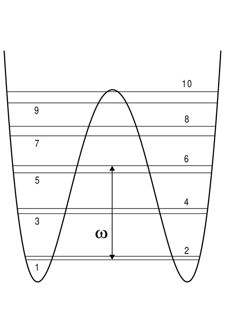
FIG. 2.: Energy diagram of the lowest lying eigenstates of a quartic double-well potential with $D=4$. The splittings of the doublets have been exaggerated for clarity.

Using convenient dimensionless variables, the corresponding Hamiltonian can be cast in the form [39]

$$H=\frac{\hat{p}^{2}}{2}-\frac{\hat{x}^{2}}{4}+\frac{\hat{x}^{4}}{64D}-\lambda\hat{x}\cos\omega t.$$ (33)

The dimensionless parameter $D$ determines the barrier height and corresponds, approximately, to the number of doublets below the top of the barrier. In the present study we take $D=4$. The frequency of the external field has been tuned to the transitions between the first and third doublets. Specifically, we have taken $\omega=(E_{6}-E_{1})$ with $E_{i}$ being the energy levels in the absence of driving field. The dimensionless field intensity $\lambda$, on the other hand, has been chosen to satisfy the strong-coupling condition $\Omega_{12}/\omega=1$, where $\Omega_{12}=\lambda\langle 1\left|\hat{x}\right|2\rangle$ (see below).

To establish a more clear connection with the formalism of the previous Sections, it is convenient to rewrite the Hamiltonian (33) in terms of a basis set $\left\{|i\rangle\right\}$ of eigenstates of the quartic oscillator. We have obtained these eigenstates numerically, by diagonalization in another truncated basis set $\left\{|\varphi_{n}\rangle\right\}$ of harmonic oscillator wave functions with a conveniently optimized frequency, following the procedure of Ref.[40]. In this way, one gains a complete knowledge of the states $|i\rangle=\sum_{n}\langle\varphi_{n}|i\rangle|\varphi_{n}\rangle$ by determining the numerical coefficients $\langle\varphi_{n}|i\rangle.$

In terms of the quartic-oscillator eigenstates, the Hamiltonian (33) takes the form

$$H=\sum_{i,j}|i\rangle\langle i|H|j\rangle\langle j|=\sum_{i}E_{i}\sigma_{ii}-\lambda\cos\omega t\sum_{i,j}\langle i|\hat{x}|j\rangle\sigma_{ij}.$$ (34)

where $\sigma_{ij}\equiv|i\rangle\langle j|$ and $E_{i}$ is the energy of state $|i\rangle$ in the absence of the periodic force. Introducing the notation $\Omega_{ij}\equiv\lambda\langle i\left|\hat{x}\right|j\rangle=\lambda\langle j\left|\hat{x}\right|i\rangle$ for the coupling constants, the connection with the formalism developed previously should now be evident.

Note that, since $\hat{x}$ is an odd operator and the parity of the quartic-oscillator eigenstate $|i\rangle$ is $(-1)^{i-1}$ (with $i=1,2,3,\ldots$), transitions between $|i\rangle\leftrightarrow|j\rangle$ are allowed only if $(i-j)$ is odd.

For a sufficiently weak driving field $\lambda$, any coupling constant $\Omega_{ij}$ will be much smaller than $\omega$ and the system will evolve in a weak-coupling regime where all of the allowed transitions are weak. Conversely, for a sufficiently intense driving field we would have $\Omega_{ij}\gg\omega$ for any $i,j$ and the system would evolve in a nonperturbative strong-coupling regime where all of the allowed transitions are strong. However, as mentioned in the Introduction, in between these two limiting cases there exists an interesting nonperturbative strong-coupling regime in which the intra-doublet transitions become strong while the corresponding inter-doublet transitions remain weak. This is so due to the fact that, in this kind of systems, the dipole matrix elements $\mu_{ij}\sim\langle i\left|\hat{x}\right|j\rangle$ between states within a given doublet turn out to be much larger than the dipole matrix elements connecting states lying in different doublets. On the other hand, under the above conditions, since inter-doublet transitions are weak, contributions coming from off-resonant doublets will be negligible, so that one expects the quartic oscillator to behave, to a good approximation, as an effective four-level system. Note, finally, that the nonperturbative regime in which we are interested lies within the range of applicability of the analytic formalism of Sec. II [see below Eq. (19)].

We have solved numerically the time-dependent Schrödinger equation corresponding to the Hamiltonian (34) by expanding its solution in the basis set of eigenstates of the quartic oscillator, and have considered as many states in the truncated basis sets so as to guarantee well-converged results. Specifically, for the physical parameters considered above, the 20 lowest-lying levels of the quartic oscillator have been included, which are more than enough to guarantee convergence. As we shall see, under the above conditions, the dynamical evolution of the system can be described, to a good approximation, by a four-level model.

In what follows we shall denote the two states of the upper doublet as $|3\rangle$ and $|4\rangle$, in accordance with the notation used in the four-level analytical model developed in the previous Section. Figure 3 shows the time evolution of the populations $\left|\langle i|\psi(t)\rangle\right|^{2}$ of the bare states $|i\rangle$ ($i=1,2,3,4$) for a system prepared in $t=0$ in the ground state. The curves plotted correspond to the numerical results obtained by solving the Schrödinger equation with the Hamiltonian (33). In Fig. 4 we show the corresponding theoretical prediction, obtained from the analytic general solution $|\psi(t)\rangle$ given by Eq. (27). It is important to note that the numerical results, unlike the analytical ones, include the contribution from all of the energy levels (and not only the contribution from the most relevant four levels). In fact, the slight discrepancy between Figs. 3 and 4 is due entirely to this circumstance, as demonstrates the fact that both analytical and numerical results become indistinguishable when the numerical problem is also restricted to the four most relevant levels.

FIG. 3.: Dimensionless time evolution of the populations of the bare states $|i\rangle$ for a system initially prepared in the ground state.

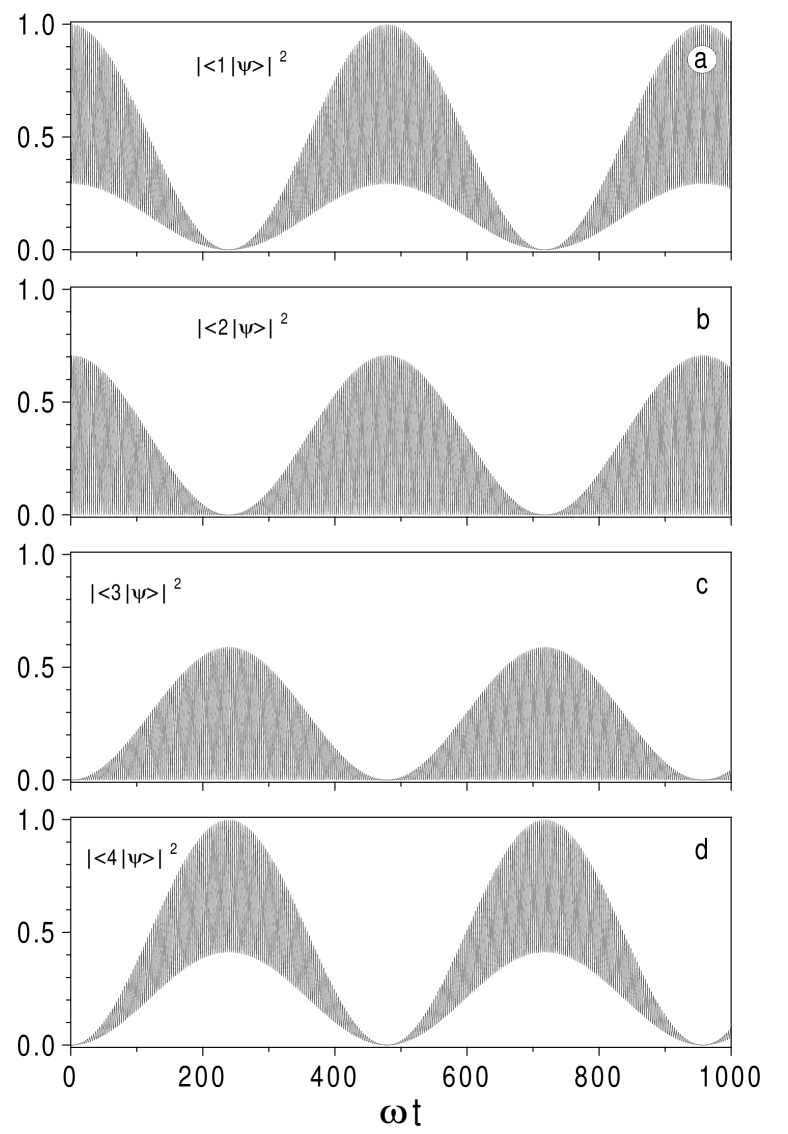
FIG. 4.: Theoretical prediction corresponding to Fig. 3.

Figures 3 and 4 show that under the action of the strong external field all of the bare states become highly populated and their time evolution couples in such a way that the population dynamics turns out to be quite different from the simple Rabi oscillations occurring in the weak-field regime. In contrast, as Fig. 5 reflects, the populations of the renormalized states $|i^{\prime}(t)\rangle$ evolve in time exhibiting the usual Rabi oscillations of the weak-field regime. Solid lines in this figure correspond to exact numerical results whereas dashed lines correspond to the analytical results obtained from Eqs. (23–26). As before, the small difference between analytical and numerical results originates from corrections to the four-level approximation. Indeed, for the high field intensity considered above, the contribution of the second and forth doublets to the dynamical evolution of the system, although small, it is not completely negligible. In fact, by monitoring the different numerical populations it can be seen that a small proportion of the populations of the first and third doublets is rapidly transferred to their corresponding adjacent doublets, giving rise to the rapid oscillations that appear superimposed to the usual Rabi oscillations in Fig. 5. When the numerical problem is restricted to the four most relevant levels this population transfer vanishes and, as already mentioned, both analytical and numerical results become indistinguishable. Since the contribution of level $|i\rangle$ to the dynamical evolution of level $|j\rangle$ is proportional to $\Omega_{ij}/\delta_{ij}$ (where $\Omega_{ij}$ is the field-dependent coupling constant between $|i\rangle$ and $|j\rangle$, and $\delta_{ij}$ is the detuning of the corresponding transition [41]), one expects a better agreement between analytical and numerical results for smaller field intensities. This is indeed the case as can be appreciated from Fig. 6. This figure shows the population dynamics of the renormalized states for an external field of the same frequency as before but a smaller field intensity, which now satisfies the strong-coupling conditions $\Omega_{12}/\omega=0.75$ (Fig. 6a) and $\Omega_{12}/\omega=0.5$ (Fig. 6b). As expected, as the intensity of the external field decreases the four-level approximation becomes more and more exact.

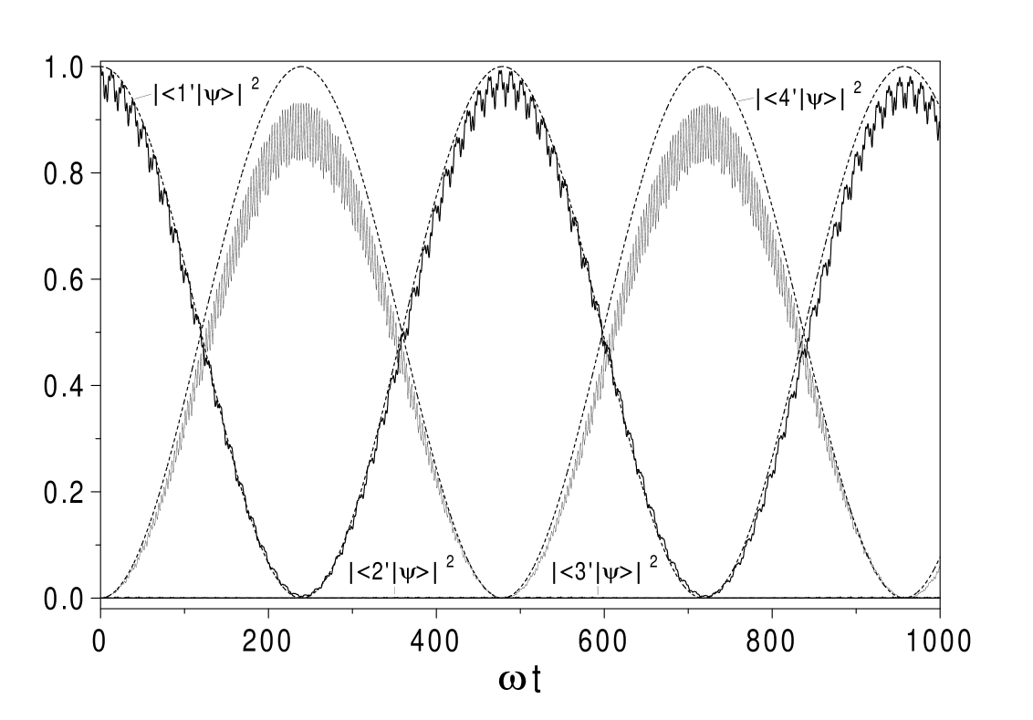
FIG. 5.: Dimensionless time evolution of the populations of the renormalized states $|i^{\prime}(t)\rangle$ for a system initially prepared in the ground state. Solid lines are exact numerical results and dashed lines are the analytical results.

Figures 5 and 6 show that, for the above initial conditions, states $|2^{\prime}(t)\rangle$ and $|3^{\prime}(t)\rangle$ remain unpopulated while the system population undergoes Rabi oscillations between the renormalized states $|1^{\prime}(t)\rangle$ and $|4^{\prime}(t)\rangle$, and this occurs in both the weak- and strong-field regimes.

FIG. 6.: The same curves as in Fig. 5 for an external field of the same frequency as before but having now an intensity satisfying the conditions (a) $\Omega_{12}/\omega=0.75$ and (b) $\Omega_{12}/\omega=0.5$.

IV Conclusion

In the nonperturbative regime the dynamical behavior of driven quantum systems becomes, in general, rather involved. In this paper we have considered an important class of driven four-level systems which are relevant in the description of numerous processes in molecular and solid-state systems, and we have shown that their nonperturbative time evolution, when analyzed in terms of a natural basis of renormalized states, essentially reduces to the corresponding time evolution in the weak-field regime, exhibiting simple Rabi oscillations between the different relevant quantum states.

Such renormalized basis enables one to absorb the nonperturbative effects induced by the strong driving field into a redefinition of the relevant energies and Rabi frequencies in such a way that the system evolves obeying the same Hamiltonian in the perturbative and nonperturbative regimes. This basis thus provides a unified description valid in both the weak- and strong-coupling regimes. In particular, in the weak-field regime, the renormalized basis becomes indistinguishable from the original one and the renormalized energies and Rabi frequencies approach their corresponding bare values, so that, in this regime, our formulation leads to the same results as the usual RWA and thus can be considered as a nonperturbative generalization of the latter.

This work has been supported by Ministerio de Ciencia y Tecnología and FEDER under Grant No. BFM2001-3343.

REFERENCES

- [1] M. Grifoni and P. Hänggi, Phys. Rep. 304, 229 (1998).
- [2] Z. Ficek and H. S. Freedhoff, in Progress in Optics, edited by E. Wolf (Elsevier, Amsterdam, 2000), p. 389.
- [3] C. J. Joachain, M. Dörr, and N. J. Kylstra, Adv. At. Mol. Phys. 42, 226 (2000).
- [4] G. Alzetta, A. Gozzini, L. Moi and G. Orriols, Nuovo Cimento B 36, 5 (1976); E. Arimondo and G. Orriols, Lett. Nuovo Cimento 17, 333 (1976); E. Arimondo, in Progress in Optics, edited by E. Wolf (Elsevier, Amsterdam, 1996), p. 257 and references therein.
- [5] V. Delgado and J. M. Gomez Llorente, Phys. Rev. Lett. 88, 053603 (2002).
- [6] S. E. Harris, Phys. Today 50, No. 7, 36 (1997).
- [7] O. Kocharovskaya and Ya. I. Khanin, JETP Lett. 48, 630 (1988); S. E. Harris, Phys. Rev. Lett. 62, 1033 (1989); A. Imamoglu, Phys. Rev. A 40, 2835 (1989); M. O. Scully et al., Phys. Rev. Lett. 62, 2813 (1989); G. S. Agarwal, Phys. Rev. A 44, R28 (1991).
- [8] J. L. Krause, K. J. Schafer, and K. C. Kulander, Phys. Rev. Lett. 68, 3535 (1992); M. Lewenstein, Ph. Balcou, M. Yu. Ivanov, A. L’Huillier, and P. B. Corkum, Phys. Rev. A 49, 2117 (1994).
- [9] Atoms in intense laser fields, edited by M. Gravila (Academic, New York, 1992).
- [10] S. H. Autler and C. H. Townes, Phys. Rev. 100, 703 (1955).
- [11] M. G. Floquet, Ann. Ecole Norm. Sup. 12, 47 (1883).
- [12] J. H. Shirley, Phys. Rev. 138, B979 (1965).
- [13] J. M. Gomez Llorente and J. Plata, Phys. Rev. A 45, R6958 (1992).
- [14] Y. Dakhnovskii and R. Bavli, Phys. Rev. B 48, 11020 (1993).
- [15] X.-G. Zhao, Phys. Rev. B 49, 16753 (1994).
- [16] M. Frasca, Phys. Rev. A 56, 1548 (1997); ibid. 60, 573 (1999).
- [17] V. Delgado and J. M. Gomez Llorente, J. Phys. B 33, 5403 (2000); A. Santana, J. M. Gomez Llorente, and V. Delgado, J. Phys. B 34, 2371 (2001).
- [18] J. C. A. Barata and W. F. Wreszinski, Phys. Rev. Lett. 84, 2112 (2000).
- [19] A. Sacchetti, J. Phys. A 34, 10293 (2001).
- [20] J. M. Gomez Llorente and J. Plata, Phys. Rev. A 49, 2759 (1994).
- [21] P. G. Burke, P. Francken, and C. J. Joachain, J. Phys. B 24, 761 (1991).
- [22] Y. Zhang, M. Ciocca, L. W. He, C. E. Burkhardt and J. J. Leventhal, Phys. Rev. A 50, 1101 (1994); ibid. 50, 4608 (1994).
- [23] M. Dörr, C. J. Joachain, R. M. Potvliege, and S. Vucic, Phys. Rev. A 49, 4852 (1994); M. Terao-Dunseath and K. M. Dunseath, J. Phys. B 35, 125 (2002).
- [24] R. Gebarowski, P. G. Burke, K. T. Taylor, M. Dörr, M. Bensaid, and C. J. Joachain, J. Phys. B 30, 1837 (1997).
- [25] S. Yoshida, C. O. Reinhold, P. Kristöfel, J. Burgdörfer, S. Watanabe, and F. B. Dunning, Phys. Rev. A 59, R4121 (1999).
- [26] W. R. Salzman, Phys. Rev. A 10, 461 (1974).
- [27] S. I. Chu and W. P. Reinhardt, Phys. Rev. Lett. 39, 1195 (1977).
- [28] S. C. Leasure, K. F. Milfeld, and R. E. Wyatt, J. Chem. Phys. 74, 6197 (1981).
- [29] R.M. Potvliege and R. Shakeshaft, in Atoms in intense laser fields, edited by M. Gravila (Academic, New York, 1992), p. 373.
- [30] M. Dörr, M. Terao-Dunseath, J. Purvis, C. J. Noble, P. G. Burke, and C. J. Joachain, J. Phys. B 25, 2809 (1992).
- [31] B. W. Shore, K. Bergmann, and J. Oreg, Z. Phys. D 23, 33 (1992).
- [32] F. Hund, Z. Phys. 43, 803 (1927).
- [33] A. Oppenländer, Ch. Rambaud, H. P. Trommsdorff, and J. C. Vial, Phys. Rev. Lett. 63, 1432 (1989).
- [34] R. Bavli and H. Metiu, Phys. Rev. Lett. 69, 1986 (1992); M. Holthaus and D. Hone, Phys. Rev. B 47, 6499 (1993); Y. Dakhnovskii, R. Bavli and H. Metiu, Phys. Rev. B 53, 4657 (1996).
- [35] R. Ferreira and G. Bastard, Rep. Prog. Phys. 60, 345 (1997).
- [36] M. Abramowitz and I. A. Stegun, Handbook of Mathematical Functions (Dover, New York, 1972).
- [37] H. Sambe, Phys. Rev. A 7, 2203 (1973).
- [38] L. I. Schiff, Quantum Mechanics (McGraw-Hill, New York, 1968).
- [39] F. Grossmann, T. Dittrich, P. Jung, and P. Hänggi, Phys. Rev. Lett. 67, 516 (1991); S. Kohler, R. Utermann, P. Hänggi, and T. Dittrich, Phys. Rev. E 58, 7219 (1998).
- [40] W. A. Lin and L. E. Ballentine, Phys. Rev. Lett. 65, 2927 (1990).
- [41] C. Cohen-Tannoudji, J. Dupont-Roc, and G. Grynberg, Atom-Photon Interactions: Basic Processes and Applications (Wiley-Interscience, New York, 1992).