Frequency up- and down-conversions in two-mode cavity quantum electrodynamics

Abstract

In this letter we present a scheme for the implementation of frequency up- and down-conversion operations in two-mode cavity quantum electrodynamics (QED). This protocol for engineering bilinear two-mode interactions could enlarge perspectives for quantum information manipulation and also be employed for fundamental tests of quantum theory in cavity QED. As an application we show how to generate a two-mode squeezed state in cavity QED (the original entangled state of Einstein-Podolsky-Rosen).

PACS numbers: 32.80.-t, 42.50.Ct, 42.50.Dv

Parametric frequency conversion has been a major ingredient in quantum optics. Employed in the generation of squeezed and two-photon states of light to test sub-poissonian statistics Stoler and Bell’s inequalities Kwiat , parametric down-conversion (PDC) has been constantly revisited through the work by Louisell et al. Louisell . Sub-poissonian statistics, one of the characteristics of squeezed light, has deepened our understanding of the properties of radiation Stoler and its interaction with matter Milburn . It has provided an unequivocal signature of the quantum nature of light, disputed since the discovery of the photoelectric effect, and has continued to motivate fundamental works up to the present Haroche . Apart from fundamental phenomena, the potential application of PDC in technology is also striking, ranging from improvements in the signal to noise ratio in optical communication SN to the possibility of measuring gravitational waves through squeezed fields Caves .

The combination of simplicity and comprehensiveness exhibited by the frequency-conversion mechanisms applied in some of the recent proposals of quantum information theory Pittman has motivated the goal of the present letter: the implementation of the frequency up- and down-conversion operations in two-mode cavity quantum electrodynamics (QED). With this protocol to engineer two-mode interactions, it would be possible to map into cavity QED some of the proposals for quantum logical processing originally designed for travelling fields. This protocol may be useful for scalable quantum computation and communication proposals CZ , besides enlarging such perspectives, it may also be employed for fundamental tests of quantum theory Rausch .

The parametric frequency conversion operations are accomplished through the dispersive interactions of the cavity modes with a single three-level-driven atom injected into the cavity, which works as a nonlinear medium. Although considerable space has been devoted in the literature to the interaction between a three-level atom and two cavity modes Walls , the issue of tailoring the bilinear Hamiltonians of frequency conversion processes in cavity QED has not been addressed.

Parametric up conversion (PUC). We envisage working with Rydberg atoms in the microwave regime. Starting with the PUC, the energy diagram of the Rydberg three-level atom is in the $\Lambda$ configuration as sketched in Fig. 1a. The ground ($\left|g\right\rangle$) and excited ($\left|e\right\rangle$) states are coupled through an auxiliary more-excited level ($\left|i\right\rangle$). The cavity microwave modes of frequencies $\omega_{a}$ and $\omega_{b}$ enable both dipole-allowed transitions $\left|g\right\rangle$ $\leftrightarrow$ $\left|i\right\rangle$ and $\left|e\right\rangle$ $\leftrightarrow$ $\left|i\right\rangle$, with coupling constants $\lambda_{a}$ and $\lambda_{b}$, respectively, and detuning $\Delta$ $=\omega_{i}-\omega_{g}-\omega_{a}=\omega_{i}-\omega_{e}-\omega_{b}$. Finally, a classical field of frequency $\omega_{0}=\omega_{e}-\omega_{g}-\delta$, dispersively driving the dipole-forbidden atomic transition $\left|g\right\rangle$ $\leftrightarrow$ $\left|e\right\rangle$ with coupling constant $\Omega$, leads to the desired interaction between the modes $\omega_{a}$ and $\omega_{b}$. This dipole-forbidden transition can be induced by applying a sufficiently strong electric field. The Hamiltonian which describe this system, in the interaction picture within the rotating wave approximation and in a rotating frame (through the unitary transformation $\exp\left[-i\Delta t\left(\sigma_{ee}+\sigma_{gg}\right)\right]$), is given by

$$\mathbf{H} =\hbar\left(\lambda_{a}a\sigma_{ig}+\lambda_{b}b\sigma_{ie}+\Omega\operatorname*{e}\nolimits^{-i\delta t}\sigma_{ge}+\mathrm{{h.c.}}\right)$$

$$-\hbar\Delta\left(\sigma_{ee}+\sigma_{gg}\right).$$ (1)

with $a^{\dagger}$ ($a$) and $b^{\dagger}$ ($b$) standing for the creation (annihilation) operators of the quantized cavity modes, while $\sigma_{kl}\equiv\left|k\right\rangle\left\langle l\right|$ $(k,l=g,e,i)$ defines the atomic transition operators.

Considering the Heisenberg equations of motion for the transition operators $\sigma_{ig}$ and $\sigma_{ei}$, we can compare the time scales of the transitions induced by the cavity modes. If the dispersive transitions induced by the quantized fields are sufficiently detuned, i.e., $\Delta\gg$ $\left|\lambda_{a}\right|$,$\left|\lambda_{b}\right|$,$\left|\Omega\right|$, we obtain the adiabatic solutions for the transition operators $\sigma_{ig}$ and $\sigma_{ie}$ by setting $d\sigma_{ig}/dt=d\sigma_{ie}/dt=0$, given by

$$\sigma_{ig} \simeq\left(\frac{\Delta^{2}}{\Delta^{2}+\Omega^{2}}\right)\left[\frac{\lambda_{a}^{\ast}}{\Delta}a^{\dagger}\left(\sigma_{ii}-\sigma_{gg}\right)-\frac{\lambda_{b}^{\ast}}{\Delta}b^{\dagger}\sigma_{eg}\right.$$

$$\left.-\frac{\Omega\lambda_{a}^{\ast}}{\Delta^{2}}\operatorname*{e}\nolimits^{-i\delta t}a^{\dagger}\sigma_{ge}+\frac{\Omega\lambda_{b}^{\ast}}{\Delta^{2}}\operatorname*{e}\nolimits^{-i\delta t}b^{\dagger}\left(\sigma_{ii}-\sigma_{ee}\right)\right],$$ (2a)

$$\sigma_{ie} \simeq\left(\frac{\Delta^{2}}{\Delta^{2}+\Omega^{2}}\right)\left[-\frac{\lambda_{a}^{\ast}}{\Delta}a^{\dagger}\sigma_{ge}+\frac{\lambda_{b}^{\ast}}{\Delta}b^{\dagger}\left(\sigma_{ii}-\sigma_{ee}\right)\right.$$

$$\left.+\frac{\Omega\lambda_{a}^{\ast}}{\Delta^{2}}\operatorname*{e}\nolimits^{i\delta t}a^{\dagger}\left(\sigma_{ii}-\sigma_{gg}\right)-\frac{\Omega\lambda_{b}^{\ast}}{\Delta^{2}}\operatorname*{e}\nolimits^{i\delta t}b^{\dagger}\sigma_{eg}\right].$$ (3a)

Inserting these adiabatic solutions for $$\sigma_{ig} \sigma_{ie} \Delta^{2}+\Omega^{2}\approx\Delta^{2}$$ and into Eq. (1), the following Hamiltonian is obtained (assuming )

$$\mathbf{H} \simeq-\hbar\left(\Delta+\frac{\left|\lambda_{b}\right|^{2}}{\Delta}\right)\sigma_{ee}-\hbar\left(\Delta+\frac{\left|\lambda_{a}\right|^{2}}{\Delta}\right)\sigma_{gg}$$

$$+\hbar\frac{\left(\left|\lambda_{a}\right|^{2}+\left|\lambda_{b}\right|^{2}\right)}{\Delta}\sigma_{ii}$$

$$+\hbar\Omega\left(1-\frac{\left(\left|\lambda_{a}\right|^{2}+\left|\lambda_{b}\right|^{2}\right)}{2\Delta^{2}}\right)\left(\operatorname*{e}\nolimits^{-i\delta t}\sigma_{ge}+\mathrm{{h.c.}}\right)$$

$$+\frac{\hbar}{\Delta}\left.\left(\left|\lambda_{a}\right|^{2}a^{\dagger}a+\left|\lambda_{b}\right|^{2}b^{\dagger}b\right)\sigma_{ii}\right]$$

$$\left.-\left|\lambda_{a}\right|^{2}a^{\dagger}a\sigma_{gg}-\left|\lambda_{b}\right|^{2}b^{\dagger}b\sigma_{ee}\right]$$

$$-\frac{\hbar\Omega}{\Delta^{2}}\left(\left|\lambda_{a}\right|^{2}a^{\dagger}a+\left|\lambda_{b}\right|^{2}b^{\dagger}b\right)\left(\operatorname*{e}\nolimits^{-i\delta t}\sigma_{ge}+\mathrm{{h.c.}}\right)$$

$$-\frac{\hbar}{\Delta}\left(\lambda_{a}\lambda_{b}^{\ast}ab^{\dagger}\sigma_{eg}+\mathrm{{h.c.}}\right)$$

$$+\frac{\hbar\Omega}{\Delta^{2}}\left(\lambda_{a}\lambda_{b}^{\ast}\operatorname*{e}\nolimits^{-i\delta t}ab^{\dagger}+\mathrm{{h.c.}}\right)\left(\sigma_{ii}-\sigma_{gg}-\sigma_{ee}\right).$$ (4)

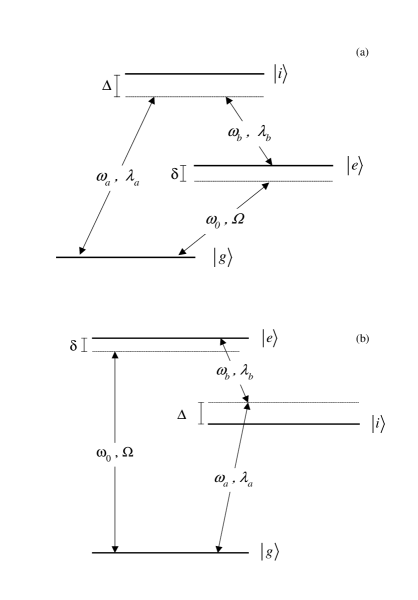
Figure 1: Energy diagram of a three-level atom in the (a) $\Lambda$ configuration to obtain the PUC process and in the (b) ladder configuration to obtain the PDC process.

The state vector associated with Hamiltonian (4), in the interaction picture, can be written as $|\Psi\left(t\right)\rangle=\sum_{\ell=g,e,i}\left|\ell\right\rangle\left|\Phi_{\ell}\left(t\right)\right\rangle\mathrm{{,}}$ where $|\Phi_{\ell}\left(t\right)\rangle=\widehat{1}_{ab}\otimes\left\langle\ell\right.|\Psi\left(t\right)\rangle$ and $\widehat{1}_{ab}$ is the unitary operator of cavity modes represented in a convenient basis. Using the orthogonality of the atomic states in $|\Psi\left(t\right)\rangle$ and Eq. (4) we obtain the uncoupled time-dependent (TD) Schrödinger equations for the atomic subspace $\left|i\right\rangle$ (in the interaction picture), $i\hbar\frac{d}{dt}|\Phi_{i}\left(t\right)\rangle=\mathcal{H}_{i}|\Phi_{i}\left(t\right)\rangle\mathrm{{,}}$ with $\mathcal{H}_{i}=\hbar\chi_{a}a^{\dagger}a+\hbar\chi_{b}b^{\dagger}b+\hbar\left(\xi\operatorname*{e}\nolimits^{-i\delta t}ab^{\dagger}+\xi^{\ast}\operatorname*{e}\nolimits^{i\delta t}a^{\dagger}b\right)\mathrm{{,}}$where $\chi_{\ell}=\left|\lambda_{\ell}\right|^{2}/\Delta$ ($\ell=a,b$) stand for the shift factors of the two cavity-mode frequencies, while $\xi=\Omega\lambda_{a}\lambda_{b}^{\ast}/\Delta^{2}$ is the effective coupling parameter between these modes. The subscript $i$ indicates the atomic subspace $\left|i\right\rangle$. The TD Schrödinger equations for subspace $\left\{\left|g\right\rangle,\left|e\right\rangle\right\}$, which follow from Eq. (4), couple the fundamental and excited atomic states. Therefore, when we prepare the initial state of the atom in the auxiliary level $\left|i\right\rangle$, the dynamics of the atom-field dispersive interactions, governed by the effective Hamiltonian $\mathcal{H}_{i}$, results in cavity modes with shifted frequencies which are coupled in identical fashion to running waves crossing a nonlinear crystal, as in PUC.

Performing a unitary transformation on the Schrödinger equation for $|\Phi_{i}\left(t\right)\rangle$, through the operator $\exp\left[-it\left(\chi_{a}a^{\dagger}a+\chi_{b}b^{\dagger}b\right)\right]$, we obtain the Hamiltonian $\widetilde{\mathcal{H}}_{i}=\hbar\left(\xi ab^{\dagger}\operatorname*{e}\nolimits^{-i\left(\delta+\chi_{a}-\chi_{b}\right)t}+\xi^{\ast}a^{\dagger}b\operatorname*{e}\nolimits^{i\left(\delta+\chi_{a}-\chi_{b}\right)t}\right)$. At this point we observe that the choice of $\delta=\left(\left|\lambda_{b}\right|^{2}-\left|\lambda_{a}\right|^{2}\right)/\Delta$, the detuning associated with the classical driving field, leads to the simplified form

$$\widetilde{\mathcal{H}}_{i}=\hbar\left(\xi ab^{\dagger}+\xi^{\ast}a^{\dagger}b\right),$$ (5)

where the up-conversion process for the effective frequencies is such that $\omega_{0}=\left(\omega_{a}+\chi_{a}\right)-\left(\omega_{b}+\chi_{b}\right)$. It should be noted that the degenerate up-conversion process is the equivalent of a beam-splitter operation, which has been generally required for quantum logical purposes Pittman .

Parametric down-conversion (PDC). Next, to engineer the PDC process, we consider the atomic levels in the ladder configuration, as shown in Fig. 1(b), where the ground and excited states are coupled through an intermediate level. The cavity microwave modes $\omega_{a}$ and $\omega_{b}$ are tuned to the vicinity of the dipole-allowed transitions $\left|g\right\rangle$ $\leftrightarrow$ $\left|i\right\rangle$ and $\left|e\right\rangle$ $\leftrightarrow$ $\left|i\right\rangle$ with coupling constants $\lambda_{a}$ and $\lambda_{b}$, respectively, and detuning $\Delta$ $=-\left(\omega_{i}-\omega_{g}-\omega_{a}\right)=\omega_{e}-\omega_{i}-\omega_{b}$. The desired interaction between the modes $\omega_{a}$ and $\omega_{b}$ is accomplished by dispersively driving  the dipole-forbidden atomic transition $\left|g\right\rangle$ $\leftrightarrow$ $\left|e\right\rangle$ with a classical field of frequency $\omega_{0}=\omega_{e}-\omega_{g}-\delta$ and coupling constant $\Omega$. The Hamiltonian to engineer the PDC, within the rotating wave approximation, is given by $H=H_{0}+V$, where

$$H_{0} =\hbar\omega_{a}a^{\dagger}a+\hbar\omega_{b}b^{\dagger}b+\sum_{\ell=g,e,i}\hbar\omega_{\ell}\sigma_{\ell\ell},$$ (6a)

$$V =\hbar\left(\lambda_{a}a\sigma_{ig}+\lambda_{b}b\sigma_{ei}+\Omega e^{i\omega_{0}t}\sigma_{ge}+\mathrm{{h.c.}}\right){.}$$ (6b)

Applying the transformation $$\exp\left[i\Delta t\left(\sigma_{ee}+\sigma_{gg}\right)\right] H \Delta\gg \left|\lambda_{a}\right| \left|\lambda_{b}\right| \left|\Omega\right|$$ to and following the steps leading from Eq. (1) to (4) (considering as in PUC case ,,), we obtain the effective Hamiltonian (in the interaction picture)

$$\mathbf{H} \simeq\hbar\left(\Delta+\frac{\left|\lambda_{a}\right|^{2}}{\Delta^{2}}\right)\sigma_{gg}+\hbar\left(\Delta+\frac{\left|\lambda_{b}\right|^{2}}{\Delta}\right)\sigma_{ee}$$

$$-\frac{\hbar\left(\left|\lambda_{a}\right|^{2}+\left|\lambda_{b}\right|^{2}\right)}{\Delta}\sigma_{ii}+\frac{\hbar}{\Delta}\left(\lambda_{a}\lambda_{b}ab\sigma_{eg}+\mathrm{{h.c.}}\right)$$

$$+\hbar\Omega\left(1-\frac{\left|\lambda_{a}\right|^{2}+\left|\lambda_{b}\right|^{2}}{2\Delta^{2}}\right)\left(e^{-i\delta t}\sigma_{ge}+\mathrm{{h.c.}}\right)$$

$$+\frac{\hbar}{\Delta}\left[-\left(\left|\lambda_{a}\right|^{2}a^{\dagger}a+\left|\lambda_{b}\right|^{2}b^{\dagger}b\right)\sigma_{ii}+\left|\lambda_{a}\right|^{2}a^{\dagger}a\sigma_{gg}+\left|\lambda_{b}\right|^{2}b^{\dagger}b\sigma_{ee}\right]$$ (7)

$$-\frac{\hbar\Omega}{\Delta^{2}}\left(\left|\lambda_{a}\right|^{2}a^{\dagger}a+\left|\lambda_{b}\right|^{2}b^{\dagger}b\right)\left(e^{-i\delta t}\sigma_{ge}+\mathrm{{h.c.}}\right)$$

$$-\frac{\hbar\Omega}{\Delta^{2}}\left(\lambda_{a}\lambda_{b}e^{-i\delta t}ab+\mathrm{{h.c.}}\right)\left(\sigma_{ee}-\sigma_{ii}+\sigma_{gg}\right).$$ (8)

Next, expanding the state vector of the system as in the PUC case and preparing the initial state of the atom in the auxiliary level, we obtain the uncoupled time-dependent (TD) Schrödinger equations for the atomic subspace $\left|i\right\rangle$, with $\mathcal{H}_{i}=-\hbar\chi_{a}a^{\dagger}a-\hbar\chi_{b}b^{\dagger}b+\hbar\left(\xi e^{-i\delta t}ab+\xi^{\ast}e^{i\delta t}a^{\dagger}b^{\dagger}\right)$, where $\xi=\Omega\lambda_{a}\lambda_{b}/\Delta^{2}$ is the effective coupling parameter between these modes. Therefore, when we prepare the initial state of the atom in the auxiliary level, the dynamics of the atom-field dispersive interactions leads to shifted cavity modes which are coupled in identical fashion to PDC. Performing the unitary transformation, $\exp\left[it\left(\chi_{a}a^{\dagger}a+\chi_{b}b^{\dagger}b\right)\right]$, we obtain the Hamiltonian $\widetilde{\mathcal{H}}_{i}=\hbar\left(\xi e^{-i\left(\delta-\chi_{a}-\chi_{b}\right)t}ab+\xi^{\ast}e^{i\left(\delta-\chi_{a}-\chi_{b}\right)t}a^{\dagger}b^{\dagger}\right).$The choice $\delta=\left(\left|\lambda_{a}\right|^{2}+\left|\lambda_{b}\right|^{2}\right)/\Delta$ leads to the simplified form (where the down-conversion process for the effective frequencies satisfies $\omega_{0}=\left(\omega_{a}-\chi_{a}\right)+\left(\omega_{b}-\chi_{b}\right)$)

$$\widetilde{\mathcal{H}}_{i}=\hbar\left(\xi ab+\xi^{\ast}a^{\dagger}b^{\dagger}\right)\mathrm{{.}}$$ (9)

Two-photon processes. We obtain from Hamiltonians (4) and (8), by switching off the classical amplification process (apart from diagonal terms), the interactions $\hbar\left(\zeta ab^{\dagger}\sigma_{eg}+\zeta^{\ast}a^{\dagger}b\sigma_{ge}\right)$ Gerry and $\hbar\left(\kappa ab\sigma_{eg}+\kappa^{\ast}a^{\dagger}b^{\dagger}\sigma_{ge}\right)$ Duvida , respectively. The coupling parameters read $\zeta=\hbar\lambda_{a}\lambda_{b}^{\ast}/\Delta$ and $\kappa=\hbar\lambda_{a}\lambda_{b}/\Delta$. With these interactions it is straightforward to prepare the Bell basis states for the cavity modes ($\left|\Psi_{ab}^{\pm}\right\rangle=\left(\left|1_{a}0_{b}\right\rangle\pm\left|0_{a}1_{b}\right\rangle\right)/\sqrt{2}$, $\left|\Phi_{ab}^{\pm}\right\rangle=\left(\left|1_{a}1_{b}\right\rangle\pm\left|0_{a}0_{b}\right\rangle\right)/\sqrt{2}$), with the passage of a single atom through the cavity. Moreover, as a by-product of the present scheme, in the case where $\omega_{a}=\omega_{b}$ (discussed in detail in Ref. Celso ) we get the degenerate PDC process corresponding to the well-known interaction $\hbar\left[\xi\left(a\right)^{2}+\xi^{\ast}\left(a^{\dagger}\right)^{2}\right]$ which has been used to generate squeezed states of light in cavity QED. We emphasize that  this degenerate down-conversion process can be used to squeeze an arbitrary state previously prepared in the cavity; i.e., to perform the operation $S\left|\Psi\right\rangle$ in cavity QED ($S$ being the squeeze operator) Celso .

The original EPR state. As another application of the present proposal, we derive the original EPR state expanded in the position representation. Starting with the two cavity modes in their vacuum states and applying the down-conversion interaction Eq. (9) during the time interval $\tau$, following the procedure described above, the evolved two-mode state reads (in the interaction picture)

$$\left|\psi(\tau)\right\rangle_{ab} =\operatorname*{e}\nolimits^{-i\tau\left(\xi ab+\xi^{\ast}a^{\dagger}b^{\dagger}\right)}\left|0,0\right\rangle_{ab}$$ (10)

$$=\sum_{n=0}^{\infty}\frac{\left[\tanh\left(\left|\xi\right|\tau\right)\right]^{n}}{\cosh\left(\left|\xi\right|\tau\right)}\left|n,n\right\rangle_{ab}\mathrm{{,}}$$ (11)

where we have adjusted the coupling constants $\lambda_{a}$ and $\lambda_{b}$ such that $\xi=i\left|\xi\right|$. This state is the two-mode squeezed vacuum state which, in the limit $\left|\xi\right|\tau\rightarrow\infty$ (and projected into the positional basis of modes $a$ and $b$), is exactly the original entanglement used in the EPR argument against the uncertainty principle EPR . In order to estimate the “quality” of the prepared EPR state (10), we compute, in this state, the mean values SB $\left(\Delta x\right)^{2}=\left\langle\left(x_{a}-x_{b}\right)^{2}\right\rangle=\left.\operatorname*{e}^{-2\left|\xi\right|\tau}\right/2$ and $(\Delta p)^{2}=\left\langle\left(p_{a}+p_{b}\right)^{2}\right\rangle=\left.\operatorname*{e}^{-2\left|\xi\right|\tau}\right/2$, where $x_{\beta}=\left(\beta+\beta^{\dagger}\right)/2$ and $p_{\beta}=-i(\beta-\beta^{\dagger})/2$ ($\beta=a,b$) are the field quadratures. We obtain the result $\left(\Delta x\right)^{2}+(\Delta p)^{2}=\operatorname*{e}\nolimits^{-2\left|\xi\right|\tau}$ which goes to zero for the ideal EPR state ($\left|\xi\right|\tau\rightarrow\infty$) and to unity for an entirely separable state SB . Therefore, the expression $1-\operatorname*{e}\nolimits^{-2\left|\xi\right|\tau}$ can be used to estimate the quality of the prepared state (10) with present-day cavity QED parameters. For specific cavity modes and atomic system, the interaction parameter $\left|\xi\right|\tau$ can be adjusted in accordance with the coupling strength $\xi$ (calculated from the parameters $\Omega$, $\lambda_{a}$, $\lambda_{b}$, and $\Delta$) and the interaction time $\tau$. Assuming typical values for the parameters involved, arising from Rydberg states where the intermediate state $\left|i\right\rangle$, an $(n-1)P_{3/2}$ level, is nearly halfway between $\left|g\right\rangle$, an $(n-1)S_{1/2}$ level, and $\left|e\right\rangle$, an $nS_{1/2}$ level, we get $\left|\lambda_{a}\right|\sim\left|\lambda_{b}\right|\sim 7\times 10^{5}$s^-1 BRH . With these values and assuming the detuning $\Delta\sim 10^{7}$s^-1 (note that $\Delta\sim 14\lambda_{a,b}$ Allen ) and the coupling strength $\Omega\sim 7\times 10^{5}$s^-1, we obtain $\left|\xi\right|\sim 3.4\times 10^{3}$s^-1. For an atom-field interaction time about $\tau\sim 2\times 10^{-4}$s, we get the interaction parameter $\left|\xi\right|\tau\sim 0.68$, close to the value ($0.69$) achieved for building the EPR state for unconditional quantum teleportation in the running-wave domain Furusawa . The value $\left|\xi\right|\tau\sim 0.68$ leads to $1-\operatorname*{e}\nolimits^{-2\left|\xi\right|\tau}$ $\sim 0.74$, and we note that increasing moderately the interaction time to $\tau\sim 6\times 10^{-4}$s ($\left|\xi\right|\tau\sim 2$) the quality of the prepared state increases to $1-\operatorname*{e}\nolimits^{-2\left|\xi\right|\tau}$ $\sim 0.98$. Regarding the degenerate PDC process ($\omega_{a}=\omega_{b}$) Celso , for an atom-field interaction time about $\tau\sim 2\times 10^{-4}$s we get the squeezing factor $r=2\left|\xi\right|\tau\sim 1.36$, such that the variance in the squeezed quadrature turns to be $\operatorname{e}^{-2r}/4\sim 1.6\times 10^{-2}$, representing a squeezing up to 93% (for an initial coherent state prepared in the cavity) with the passage of just one atom.

There are some sensitive points in the experimental implementation of the present scheme. The atomic detection efficiency and the spread of the atomic velocity do not play important roles in the present scheme were only one step of atom-fields interactions is required. However, due to the Gaussian profile $f(x)$ of the cavity fields in the transverse direction, the atom-field couplings $\lambda_{a}$ and $\lambda_{b}$ become time-dependent parameters as well as the effective coupling between the cavity modes $\xi=\Omega\lambda_{a}\lambda_{b}\left[f(x)\right]^{2}/\Delta^{2}$ (where $f(x)=\exp(-x^{2}/w^{2})$, $x$ is the time-dependent atom position from the center of the cavity, and $w\sim 0.6$ cm Haroche01 is the waist of the Gaussian). The effect of the field profile can be evaluated straightforward by using the analytical results for a time-dependent degenerate PDC process, demonstrated in Celso01 , leading to the squeezing factor $r=\left(\left.\Omega\lambda_{a}\lambda_{b}\right/\Delta^{2}\right)2\int_{0}^{\tau}\left[f(x)\right]^{2}dt$. Considering the atom-field interaction time about $\tau\sim 2\times 10^{-4}$s, we get the squeezing factor $r\sim 0.51$. To obtain the same value $r\sim 1.36$ of the ideal case, we must increase moderately the interaction time to $\tau\sim 5.32\times 10^{-4}$s. The interaction times cited above are at least one order of magnitude smaller than the decay time of the open cavities used in cavity QED experiments Rausch ; Haroche01 . Regarding atomic decay, we note that for Rydberg levels the damping effects can be safely neglected for typical interaction time scales.

We note that, to characterize the entangled state in (10) we can use the reconstruction technique presented in FLD . To employ this technique we have firstly to apply the displacement operator $D^{-1}(\eta_{\ell},\eta_{\ell}^{\ast})=\exp(-\eta_{\ell}\ell^{\dagger}+\eta_{\ell}^{\ast}\ell)$, with $\ell=a,b$, into the cavity modes. Next, an additional three-level atom is sent through the cavity, prepared in the superposition state $\left(\left|i\right\rangle+\left|f\right\rangle\right)/\sqrt{2}$, where $\left|f\right\rangle$ stands for an auxiliary Rydberg level whose transitions to the states $\left|g\right\rangle$, $\left|i\right\rangle$, and $\left|e\right\rangle$ do not couple to the cavity modes. Turning off the classical amplification field and considering the atom-fields interaction time $t$, we obtain from Hamiltonian (8), the evolved state $\left[\exp\left[i\phi\left(a^{\dagger}a+b^{\dagger}b\right)\right]\left|\psi(\tau)\right\rangle_{ab}\left|i\right\rangle+\left|\psi(\tau)\right\rangle_{ab}\left|f\right\rangle\right]/\sqrt{2}$ where $\phi=\left|\lambda\right|^{2}t/\Delta$ ($\left|\lambda\right|=\left|\lambda_{a}\right|\sim\left|\lambda_{b}\right|$). After undergoing a $\pi/2$ pulse in a Ramsey zone, with phase chosen so that $\left|i\right\rangle\rightarrow\left(\left|i\right\rangle+\left|f\right\rangle\right)/\sqrt{2}$ and $\left|f\right\rangle\rightarrow\left(\left|i\right\rangle-\left|f\right\rangle\right)/\sqrt{2}$, the atomic states $\left|i\right\rangle$ and $\left|f\right\rangle$ are measured with probabilities $\mathcal{P}_{i}$ and $\mathcal{P}_{f}$. Finally, the direct measurement of the two-mode Wigner function follows from $W(\eta_{a},\eta_{b},\eta_{a}^{\ast},\eta_{b}^{\ast})\varpropto\mathcal{P}_{f}-\mathcal{P}_{i}$ FLD . In the particular case of degenerated parametric down-convention, where the resulting Hamiltonian is the squeezing operator of a single cavity mode, the same scheme can be used to measure directly the Wigner function of any squeezed state.

References

• (1) D. Stoler, Phys. Rev. Lett. 33, 1397 (1974).
• (2) P. G. Kwiat, et al., Phys. Rev. Lett. 75, 4337 (1995).
• (3) W. H. Louisell, A. Yariv, and A. E. Siegman, Phys. Rev. 124, 1646 (1961).
• (4) G. J. Milburn, Opt. Acta. 31, 671 (1984); H. J. Kimble, M. Dagenais, and L. Mandel, Phys. Rev. Lett. 39, 691 (1977); H. P. Yuen and J. H. Shapiro, Opt. Lett. 4, 334 (1979).
• (5) M. Brune, et al., Phys. Rev. Lett. 76, 1800 (1996); D. M. Meekhof, et al., ibid. 76, 1796 (1996); Ch. Roos, et al., ibid. 83, 4713 (1999).
• (6) H. P. Yuen and J. H. Shapiro, IEEE Trans. Inf. Theory 24, 657 (1978); D. J. Wineland, J. J. Bollinger, W. M. Itano, and D. J. Heinzen, Phys. Rev. A 50, 67 (1994).
• (7) J. N. Hollenhorst, Phys. Rev. D 19, 1669 (1979); C. M. Caves, et al., Rev. Mod. Phys. 52, 341 (1980).
• (8) E. Knill, R. Laflamme, and G. J. Milburn, Nature 409, 46 (2001); T. B. Pittman, B. C. Jacobs, and J. D. Franson, Phys. Rev. Lett. 88, 257902 (2002).
• (9) J. I. Cirac and P. Zoller, Phys. Rev. Lett. 74, 4091 (1995); T. Pellizzari, ibid. 79, 5242 (1997); S. Lloyd, M. S. Shahriar, J. H. Shapiro, and P. R. Hemmer, ibid. 87, 167903 (2001).
• (10) A. Rauschenbeutel, et al., Phys. Rev. A 64, 050301(R) (2001); B. T. H. Varcoe, S. Brattke, M. Weidinger, H. Walther, Nature 403, 743 (2000).
• (11) A. Einstein, B. Podolsky, and N. Rosen, Phys. Rev. 47, 777 (1935).
• (12) C. A. Blockley and D. F. Walls, Phys. Rev. A, 43, 5049 (1991); N. A. Ansari, J. Gea–Banacloche, and M. S. Zubairy, ibid. 41, 5179 (1990); B. J. Dalton, Z. Ficek, and P. L. Knight, ibid. 50, 2646 (1994).
• (13) C. C. Gerry and J. H. Eberly, Phys. Rev. A 42, 6805 (1990).
• (14) S. C. Gou, Phys. Rev. A 40, 5116 (1989).
• (15) C. J. Villas-Bôas, N. G. de Almeida, R. M. Serra, and M. H. Y. Moussa, Phys. Rev. A 68, 061801(R) (2003).
• (16) S. L. Braunstein,C. A. Fuchs, H. J. Kimble, and P. van Loock , Phys. Rev. A 64, 022321 (2001).
• (17) M. Brune, J. M. Raimond, and S. Haroche, Phys. Rev. A 35, 154 (1987).
• (18) For the typical parameters mentioned here, with $\Delta\sim 14\lambda_{a,b}$, we have a deviation from unity about 3%, for $\left\langle\sigma_{ii}\right\rangle(t)$, when considering a numerical simulation with Hamiltonian (1). A carefull analyses, including numerical simulations, will be present elsewhere. A similar discussion has been done in Ref. X. X. Yi, et al, e-print quant-ph/0306035.
• (19) A. Furasawa, et al., Science 282, 706 (1998); E. S. Polzik, J. Carri, and H. J. Kimble, Phys. Rev. Lett. 68, 3020 (1992).
• (20) S. Osnaghi, et al., Phys. Rev Lett. 87, 037902 (2001).
• (21) C. J. Villas-Bôas, F. R. de Paula, R. M. Serra, and M. H. Y. Moussa, Phys. Rev. A 68, 053808 (2003).
• (22) M. França Santos, L. G. Lutterbach, and L. Davidovich, J. Opt. B: Quantum Semiclass. Opt. 3, S55 (2001); L. G. Lutterbach and L. Davidovich, Phys. Rev. Lett. 78, 2547 (1997).