Gaussian resolutions for equilibrium density matrices

Abstract

A Gaussian resolution method for the computation of equilibrium density matrices $\widehat{\rho}_{T}$ for a general multidimensional quantum problem is presented. The variational principle applied to the “imaginary time” Schrödinger equation provides the equations of motion for Gaussians in a resolution of $\widehat{\rho}_{T}$ described by their width matrix, center and scale factor, all treated as dynamical variables. The method is computationally very inexpensive, has favorable scaling with the system size and is surprisingly accurate in a wide temperature range, even for cases involving quantum tunneling. Incorporation of symmetry constraints, such as reflection or particle statistics, is also discussed.

Propagating Gaussian resolutions. Computing the equilibrium quantum density matrix

$$\widehat{\rho}_{T}:=Z^{-1}e^{-\beta\widehat{H}},~{}~{}~{}Z:=\mbox{Tr~{}}e^{-\beta\widehat{H}},$$ (1)

in dependence of the inverse temperature $\beta=1/kT$, or finding an equilibrium property of the type

$$\langle\widehat{A}\rangle_{T}:=\mbox{Tr~{}}\widehat{\rho}_{T}\widehat{A}$$ (2)

for some operator $\widehat{A}$, is of great interest in statistical physics and molecular dynamics. The most accurate methods, based on a spectral resolution

$\displaystyle\widehat{\rho}_{T}=\sum_{n}e^{-\beta E_{n}}|n\rangle\langle n|$

are extremely expensive and limited to very few degrees of freedom. Commonly used practical, albeit still very expensive, strategies involve path integrals [1]. An alternative semiclassical method was recently proposed [2], but it is also expensive, while not very accurate. In this letter we modify the Gaussian propagation techniques of solving the time-dependent Scrödinger equation [3, 4, 5, 6] for the present case, formally corresponding to propagation in imaginary time $\beta$, and complement it by an important new idea: Monte Carlo-type sampling is replaced by the propagation of a Gaussian resolution of $\widehat{\rho}_{T}$. This brings our semiclassical technique formally closer to the full quantum treatment by a spectral resolution. It turns out to give a simple, very inexpensive and surprisingly accurate alternative to the other approaches. An extension to nonequilibrium problems is possible and will be discussed elsewhere. Consider a $N$-body (or $D=3N$-dimensional) quantum system with Hamiltonian

$$\widehat{H}=\frac{1}{2}\widehat{p}^{\rm T}M^{-1}\widehat{p}+U(x).$$ (3)

Here $\widehat{p}$ ($x$) define $D$-dimensional column vectors of momentum (coordinate) operators and $M$ is the mass matrix. The potential function $U(x)$ is assumed to be representable as a sum of terms, each being a product of a complex Gaussian times a polynomial. (With this assumption a commonly used plane wave representation of $U(x)$ is covered.) Given a grid $q_{n}$ spanning the physically relevant region in configuration space we put

$$|q_{n,\tau}\rangle:=e^{-\tau\widehat{H}}|q_{n}\rangle,$$ (4)

with $\langle x|q_{n}\rangle=\delta(x-q_{n})$. The resolution of identity can be approximated by

$$\widehat{I}=\int\,d^{\rm D}q\,|q\rangle\langle q|\approx\sum_{n}w_{n}\,|q_{n}\rangle\langle q_{n}|,$$ (5)

where the sum is over all the grid points and the $w_{n}$ are quadrature weights defined by the inverse local density of $q_{n}$. (For large number of dimensions $D$ a Monte Carlo procedure to generate $q_{n}$ may be adopted.) Writing $e^{-\beta\widehat{H}}=e^{-\beta\widehat{H}/2}\widehat{I}e^{-\beta\widehat{H}/2}$ and inserting Eq. 5, we obtain

$$Z\approx\sum w_{n}\langle q_{n,\beta/2}|q_{n,\beta/2}\rangle,$$ (6)

$$\widehat{\rho}_{T}\approx Z^{-1}\sum w_{n}|q_{n,\beta/2}\rangle\langle q_{n,\beta/2}|,$$ (7)

To find $|q_{n,\beta/2}\rangle$ we note that it is the solution of the initial-value problem

$$\frac{d}{d\tau}|q_{n,\tau}\rangle=-\widehat{H}|q_{n,\tau}\rangle,~{}~{}~{}|q_{n,0}\rangle=|q_{n}\rangle$$ (8)

We solve Eq.(8) approximately using the ansatz [3, 4, 5, 6]

$$|q_{n,\tau}\rangle\approx|\lambda(\tau)\rangle$$ (9)

with

$$\langle x|\lambda(\tau)\rangle=\exp\left\{\gamma(\tau)-{1\over 2}[x-q(\tau)]^{T}G(\tau)[x-q(\tau)]\right\}.$$ (10)

This is a Gaussian with center $q$, a real vector, width matrix $G$, a real symmetric and positive definite, and scale $\gamma$, a real constant, and $\lambda:=(G,q,\gamma)$, a short-cut notation containing all the Gaussian parameters. With this ansatz the maximum number of parameters corresponding to the use of full $D\times D$ dimensional matrix $G$ is $(D+2)(D+1)/2$. This number may possibly be reduced assuming weak coupling between certain degrees of freedom and setting the corresponding matrix elements of $G$ to zero. The minimum number of $2D+1$ parameters would correspond to using a diagonal width matrix $G$. To solve for $\lambda=\lambda(\tau)$ we follow the corresponding derivations [3, 4, 5, 6] for the real-time dynamics of a Gaussian wavepacket by utilizing the variational principle

$$\left[{\partial L\over\partial\lambda^{\prime}}\right]_{\lambda^{\prime}=\lambda}=0$$ (11)

with the Lagrangian

$$L=\left\langle\lambda^{\prime}(\tau)\left|{d\over d\tau}+\widehat{H}\right|\lambda(\tau)\right\rangle.$$ (12)

Defining the two matrices

$$K=\langle\lambda^{\prime}|\lambda\rangle,~{}~{}~{}H=\langle\lambda^{\prime}|\widehat{H}|\lambda\rangle,$$ (13)

Eq. 11 can be rewritten as

$$\left[\frac{\partial^{2}K}{\partial\lambda\partial\lambda^{\prime}}\dot{\lambda}+\frac{\partial H}{\partial\lambda^{\prime}}\right]_{\lambda^{\prime}=\lambda}=0,$$ (14)

thus providing the equations of motion for the Gaussian parameters $\lambda=\lambda(\tau)$. The use of the Gaussian wavepackets and the assumed form of the Hamiltonian (3) allows one to evaluate the corresponding matrix elements and their derivatives in Eq. 14 analytically. (Efficient numerical expressions will be published elsewhere, but see refs. [4, 6]). Note that the commonly used linearization of the potential [3] reduces the complexity of the matrix elements evaluation, but also the accuracy, and is not used here. The delta function in the initial condition of Eq.(8) can be considered as a limit of the Gaussian (10) with infinite $G$. To avoid the singularities at $\tau=0$ we start instead at some small $\tau_{0}$ where we approximate $|q_{n,\tau_{0}}\rangle$ by a Gaussian that has finite width:

$$\langle x|\lambda(\tau_{0})\rangle \approx \sqrt{\frac{\det M}{(2\pi\tau_{0})^{d}}}$$ (15)

$$\times \exp\left[-\frac{1}{2\tau_{0}}(x-q_{n})^{T}M(x-q_{n})-U(q_{n})\tau_{0}\right].$$ (16)

To solve Eq. 14, we use the implicit integrator DASSL [7], which has an error control and can be applied directly to Eq. 14. (Probably, a standard numerical integrator could be utilized, if Eq. 14 is explicitly solved for $\dot{\lambda}$.) Note that $\beta$ is small at large temperature $kT=1/\beta$, and only a few integration steps are needed. As $T$ decreases, the integration time becomes larger, and the variational approximation by Gaussians may become poorer. We did not encounter any special numerical difficulties, except in the cases when the Gaussian width was too small. Given (9), we can rewrite (7) as

$$\widehat{\rho}_{T}\approx Z^{-1}\sum w_{n}|\lambda_{n}(\beta/2)\rangle\langle\lambda_{n}(\beta/2)|,$$ (17)

and get for expectations

$$\langle A\rangle_{T}\approx Z^{-1}\sum w_{n}\langle\lambda_{n}(\beta/2)|\widehat{A}|\lambda_{n}(\beta/2)\rangle.$$ (18)

The evaluation of $\langle A\rangle$ requires the computation of many matrix elements of $\widehat{A}$ between new Gaussian wavepackets for every value of $T$. This can be done analytically if $A$ is polynomial in $p,x$ or the product of a polynomial and a complex Gaussian.

Taking into account symmetry. Very often the system in question has symmetries, that is, the corresponding time-dependent Schrödinger equation conserves certain symmetries. To show how to utilize this, we consider the example of reflection symmetry, $\widehat{S}\psi(x)=\psi(-x)$, and assume that

$$|q_{n,\tau}^{\pm}\rangle={1\over\sqrt{2}}(|q_{n,\tau}\rangle\pm\widehat{S}|q_{n,\tau}\rangle)$$ (19)

is a solution of Eq. 8 at any $\tau$. Rewriting the resolution of identity,

$$\widehat{I}\approx\sum_{n}w_{n}(|q_{n}^{+}\rangle\langle q^{+}_{n}|+|q_{n}^{-}\rangle\langle q^{-}_{n}|),$$ (20)

we obtain

$$Z \approx \sum w_{n}(\langle q_{n,\beta/2}^{+}|q_{n,\beta/2}^{+}\rangle+\langle q_{n,\beta/2}^{-}|q_{n,\beta/2}^{-}\rangle),$$ (21)

$$\widehat{\rho} \approx Z^{-1}\sum w_{n}(|q_{n,\beta/2}^{+}\rangle|\langle q_{n,\beta/2}^{+}|+|q_{n,\beta/2}^{-}\rangle|\langle q_{n,\beta/2}^{-}|),$$ (22)

$$\langle A\rangle \approx Z^{-1}\sum w_{n}(\langle q_{n,\beta/2}^{+}|\widehat{A}|q_{n,\beta/2}^{+}\rangle+\langle q_{n,\beta/2}^{-}|\widehat{A}|q_{n,\beta/2}^{-}\rangle).$$ (23)

To approximate the solutions $|q_{n,\tau}^{\pm}\rangle$ we can replace the Gaussian in Eq. 9 by the symmetrized Gaussian:

$$|\lambda_{\pm}\rangle={1\over\sqrt{2}}(|\lambda\rangle\pm\widehat{S}|\lambda\rangle),$$ (24)

where

$$\widehat{S}|G(\tau),q(\tau),\gamma(\tau)\rangle=|G(\tau),-q(\tau),\gamma(\tau)\rangle.$$

Therefore, the matrix elements needed in Eq. 14 can be evaluated by taking the appropriate linear combinations of matrix elements between single Gaussians.

Bose and Fermi statistics. Another important case of symmetry corresponds to the Bose or Fermi statistics. For a system of $N$ indistinguishable particles in configuration space defined by the coordinates

$$x=(x_{1},\dots,x_{N})^{\rm T}$$

we should symmetrize or antisymmetrize the wavepackets according to the particle statistics. Let $\alpha=(\alpha_{1},\dots,\alpha_{N})$ define a permutation of particle indices, and denote by $P_{\alpha}$ the permutation matrix with

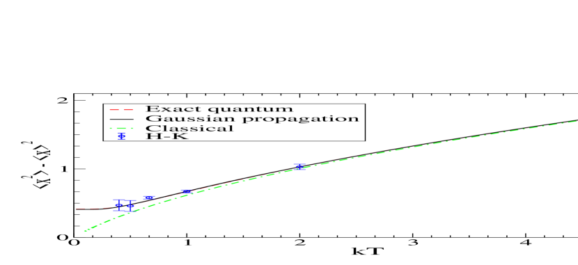
FIG. 1.: Mean square displacement computed by four different methods for 1D single well potential $U(x)={1\over 2}x^{2}+0.1x^{4}$. The semiclassical result labeled by “H-K” is taken from ref.1 The difference between the present and exact quantum result is not seen in the graph.

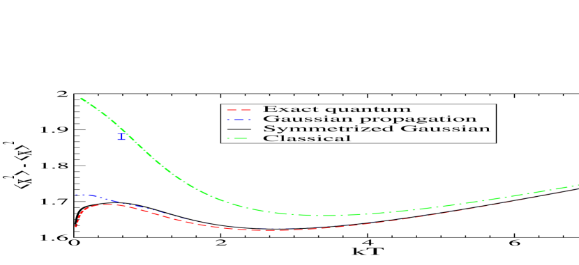
FIG. 2.: The mean square displacement for the symmetric double-well potential $U(x)=4-4x^{2}+x^{4}$ computed by four different methods.

$$P_{\alpha}x=(x_{\alpha_{1}},\dots,x_{\alpha_{N}})^{\rm T}.$$

A symmetrized wavepacket $|\lambda_{\pm}\rangle$ can be defined by

$$\langle x|\lambda_{\pm}\rangle=\sum_{\alpha}\mbox{sign}_{\pm}(\alpha)\langle P_{\alpha}x|\lambda\rangle.$$ (25)

Here boson statistics has $\mbox{sign}_{-}(\alpha)=1$; in the case of fermion statistics, $\mbox{sign}_{+}(\alpha)=1$ for even permutations and $\mbox{sign}_{+}(\alpha)=-1$ for odd permutations. The equations of motion (14) have the same general form. Since Eq. 25 implies

$\displaystyle|\lambda_{\pm}\rangle=\sum_{\alpha}\mbox{sign}_{\pm}(\alpha)P_{\alpha}^{*}|\lambda\rangle$

and one easily verifies

$\displaystyle P_{\alpha}^{*}|G,q,\gamma\rangle=|P_{\alpha}^{*}GP_{\alpha},P_{\alpha}^{*}q,\gamma\rangle,$

here again, matrix elements with symmetrized Gaussians $|\lambda_{\pm}\rangle$ are simple linear combinations of suitable matrix elements with unsymmetrized Gaussians. Similar considerations apply to multiparticle systems with few indistinguishable particles, where the sum(25) has only a few terms and the calculations remain feasible.

Numerical examples

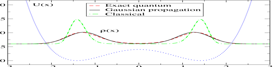
FIG. 3.: The density $\rho(x)=\langle x|\widehat{\rho}|x\rangle$ at $kT=0.5$ computed by three different methods for the symmetric double-well potential $U(x)$ as in Fig. 2.

1D single-well problem. We first apply the method to a 1D problem of ref. [2] with potential $U(x)={1\over 2}x^{2}+0.1x^{4}$ to compute the mean square displacement $\langle x^{2}\rangle-\langle x\rangle^{2}$ as a function of temperature $T$. A grid of 10 equidistant points was taken in the interval $-5<q_{n}<5$. (Here and in all the following examples the reported results fully converged with respect to the grid size.) Each of the 10 Gaussians was then propagated by Eq. 14 starting with $\tau_{0}=0.01$ up to $\tau=50$. The result obtained by the present method is hardly distinguishable from the converged quantum calculation using diagonalization of the Hamiltonian in a large basis. In Fig. 1 these results are also compared to the classical Boltzmann average and to the semiclassical calculation using the Herman-Kluk propagator [2]. Note that in the latter case a much more expensive Monte Carlo method was used with $10^{5}$ classical trajectories, still resulting in relatively big statistical errors.

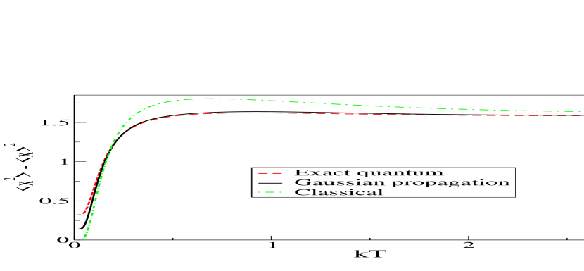
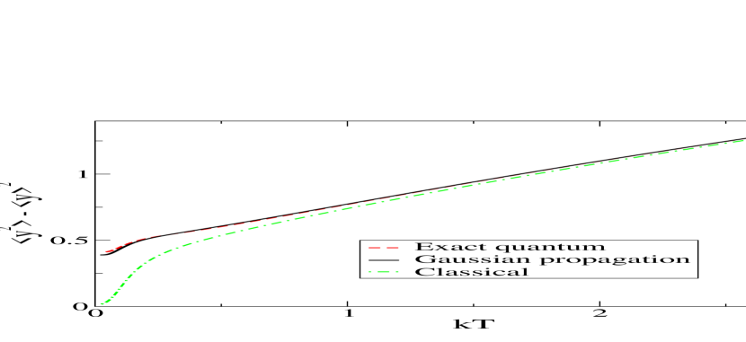
FIG. 4.: The mean square displacements computed by three different methods for the asymmetric 2D double-well potential $U(x,y)=(x^{2}-2)^{2}+0.1x+0.5(y-0.5x)^{2}+0.1y^{4}$

We note that a similar high accuracy was achieved for a 2D single well problem (not shown here).

1D symmetric double-well problem. Here the method was applied to a problem with the potential $U(x)=4-4x^{2}+x^{4}$. Now a grid of 14 points with $-3<q_{n}<3$ was used. The corresponding results using both the unsymmetrized and symmetrized gaussians are shown in Fig. 2. The agreement between the exact result (fully converged diagonalization of $\widehat{H}$ in a large basis) and that computed by the present method is unexpectedly excellent even at quite low temperatures, well below the potential barrier. For the unsymmetrized case a significant deviation from the exact (and symmetrized) result occurs only at low temperatures where the small tunneling splitting causes the quantum observables change rapidly with $T$. In Fig. 3 we show the density profile for the same system computed using the same set of 14 symmetrized Gaussians at $kT=0.5$ together with the exact quantum and classical results.

2D asymmetric double-well problem. To further demonstrate the method we apply it to a 2D problem with asymmetric double-well potential $U(x,y)=(x^{2}-2)^{2}+0.1x+0.5(y-0.5x)^{2}+0.1y^{4}$. An equidistant $16\times 16$ grid $q_{n}$ in a square box $[-4;4]\times[-4;4]$ was used. The results for the mean square displacements shown in Fig. 4 are again surprisingly accurate, except for very low temperatures.

Acknowledgement.     V.A.M. acknowledges the NSF support, grant CHE-0108823. He is an Alfred P. Sloan research fellow.

REFERENCES

- [1] R. P. Feynman and A. R. Hibbs, Quantum mechanics and path integrals, McGrow-Hill, New York (1965).
- [2] N. Makri and W. H. Miller, J. Chem. Phys. 116, 9207 (2002).
- [3] E. J. Heller, J. Chem. Phys. 62, 1544 (1975).
- [4] A. I. Sawada, R. H. Heather, B. Jackson, and H. Matiu, J. Chem. Phys. 83, 3009 (1985).
- [5] R. D. Coalson and M. Karplus, J. Chem. Phys. 93, 3919 (1990).
- [6] A. K. Pattanayak, W. C. Schieve, Phys. Rev. E 50, 3601 (1994).
- [7] L. R. Petzold, A description of DASSL: A differential/algebraic system solver, in Scientific Computing, eds. R. S. Stepleman et al., North- Holland, Amsterdam (1983), 65–68.