The moduli space of three qutrit states

Abstract

We study the invariant theory of trilinear forms over a three-dimensional complex vector space, and apply it to investigate the behaviour of pure entangled three-partite qutrit states and their normal forms under local filtering operations (SLOCC). We describe the orbit space of the SLOCC group $SL(3,{\mathbb{C}\,})^{\times 3}$ both in its affine and projective versions in terms of a very symmetric normal form parameterized by three complex numbers. The parameters of the possible normal forms of a given state are roots of an algebraic equation, which is proved to be solvable by radicals. The structure of the sets of equivalent normal forms is related to the geometry of certain regular complex polytopes.

I Introduction

The invariant theory of trilinear forms over a three-dimensional complex vector space is an old subject with a long history, which, as we shall see, appears even longer if we take into account certain indirect but highly relevant contributions Maschke (1889); Orlik and Solomon (1982); Shephard and Todd (1954); Coxeter (1940). This question has been recently revived in the field of Quantum Information Theory as the problem of classifying entanglement patterns of three-qutrit states.

Indeed, since the advent of quantum computation and quantum cryptography, entanglement has been promoted to a resource that allows quantum physics to perform tasks that are classically impossible. Quantum cryptography Bennett and Brassard (1984); Ekert (1991) proved that this gap even exists with small systems of two entangled qubits. Furthermore, it is expected that the study of higher dimensional systems and of multipartite (e.g. 3-partite) states would lead to more applications. A seminal example is the so-called 3-qutrit Aharonov-state, which “is so elegant it had to be useful”Fitzi et al. (2001): Fitzi, Gisin and Maurer Fitzi et al. (2001) found out that the classically impossible Byzantine agreement problem Lamport et al. (1982) can be solved using 3-partite qutrit states. From a more fundamental point a view, the Aharonov state led to non-trivial counterexamples of the conjectures on additivity of the relative entropy of entanglement Vollbrecht and Werner (2001) and of the output purity of quantum channels Werner and Holevo (2002). Obviously, these results provide a strong motivation for studying 3-partite qutrit states. Furthermore, interesting families of higher-dimensional states are perfectly suited to address questions concerning local realism and Bell inequalities (see e.g. Kaszlikowski et al. (2002) for a study of three-qutrit correlations).

It is therefore of interest to find some classification scheme for three-qutrit states. A possible direction is to look for classes of equivalent states, in the sense that they are equivalent up to local unitary transformations Acín et al. (2000); Carteret et al. (2000); Verstraete et al. (2001) or local filtering operations (also called SLOCC operations) Dür et al. (2000); Verstraete et al. (2001); Klyachko (2002); Verstraete et al. (2002); Luque and Thibon (2003). In the case of three qubits, especially the last classification proved to yield a lot of insights (the classification up to local unitaries has too much parameters left); the reason for that is that in the closure of each generic orbit induced by SLOCC operations, there is a unique state (up to local unitary transformations) with maximal entanglement Verstraete et al. (2001); Klyachko (2002).

In Verstraete et al. (2002), a numerical method converging to such a maximally entangled state has been described. It has been experimentally observed that, when applied to a three qutrit state, this method converged to a very special normal form. We shall provide a formal proof of this property, and then study in some detail the geometry of those normal forms. Precise statements of the results are summarized in the forthcoming section.

II Results

Let $V={\mathbb{C}\,}^{3}$ and ${\cal H}=V\otimes V\otimes V$ regarded as a representation of the group $G=SL(3,{\mathbb{C}\,})^{\times 3}$. The elements of ${\cal H}$ will be interpreted either as three-qutrit states

$$|\psi\rangle=\sum_{i,j,k=1}^{3}A_{ijk}|i,j,k\rangle$$ (1)

or as a trilinear forms

$$f=f({\bf x},{\bf y},{\bf z})=\sum_{i,j,k=1}^{3}A_{ijk}x_{i}y_{j}z_{k}$$ (2)

that is, we identify the basis state $|ijk\rangle$ with the monomial $x_{i}y_{j}z_{k}$. If $g=(g^{(1)},g^{(2)},g^{(3)})\in G$ is a triple of matrices, we define $x^{\prime}_{i}=\sum_{p}g_{ip}^{(1)}x_{p}$, $y^{\prime}_{j}=\sum_{q}g_{jq}^{(2)}y_{q}$,$z^{\prime}_{k}=\sum_{r}g_{kr}^{(3)}x_{r}$, and the coefficients $A^{\prime}_{ijk}$ by the condition

$$\sum A_{ijk}^{\prime}x^{\prime}_{i}y^{\prime}_{j}z^{\prime}_{k}=\sum A_{ijk}x_{i}y_{j}z_{k},$$ (3)

the action of $G$ on $\cal H$ being defined by

$$g\cdot f=\sum A^{\prime}_{ijk}x_{i}y_{j}z_{k}$$ (4)

It has been shown by Vinberg Vinberg (1975) that a generic state can be reduced to the normal form

$$A^{\prime}_{ijk}=u\delta_{ijk}+{w-v\over 2}\epsilon_{ijk}+{w+v\over 2}|\epsilon_{ijk}|$$ (5)

(where $\delta_{ijk}$ is the Kronecker symbol and $\epsilon_{ijk}$ the completely antisymetric tensor) by an appropriate choice of $g\in G$.

Our first result is

Theorem II.1

When applied to a generic $3$-qutrit state (1) the numerical algorithm of Verstraete et al. (2002) converges to a state which is a Vinberg normal form, generically in the same $G$-orbit as $|\psi\rangle$.

As proved in Verstraete et al. (2002, 2001), the normal form $|\psi^{\prime}\rangle$ is unique up to local unitary transformations. More precisely,

Theorem II.2

A generic state has exactly $648$ different normal forms. For special states, this number can be reduced to $216$, $72$, $27$ or $1$. Moreover, the coefficients $u$, $v$, $w$ of the normal form can be computed algebraically.

Theorem II.3

The coefficients of the normal forms are determined, up to a sign, by an algebraic equation of degree $1296$, which is explicitly solvable by radicals.

To form this equation, we need some notions of invariant theory.

A polynomial $P(A)$ in the coefficients $A_{ijk}$ is an invariant of the action of $G$ on $\cal H$ if $P(A^{\prime})=P(A)$ for all $g\in G$. These invariants form a graded algebra $R$ (any invariant $P$ is a sum of homogeneous invariants) and the first issue is to determine the dimension of the space $R_{d}$ of homogeneous invariant of degree $d$. The Hilbert series

$$h(t)=\sum_{d\geq 0}\dim R_{d}t^{d}$$ (6)

is known Vinberg (1975)

$$h(t)={1\over(1-t^{6})(1-t^{9})(1-t^{12})}$$ (7)

and in fact, one can prove that $R$ is a polynomial algebra generated by three algebraically independent invariants of respective degree $6$, $9$ and $12$.

The modern way to prove this result is due to Vinberg, who obtained it from his notion of Weyl group of a graded Lie algebra, applied to a $Z_{3}$-grading of the exceptional Lie algebra $E_{6}$ Vinberg (1976).

In section III, we shall explain how it can be deduced from the work of Chanler Chanler (1939). We prove that certain invariants $I_{6}$, $I_{9}$ and $I_{12}$ introduced in Ref. Chanler (1939) are indeed algebraic generators of $R$ and explain how to compute them from the numerical values of the coefficients $A_{ijk}$, by expressing them in terms of transvectants, that is, by means of certain differential polynomials in the form $f$, rather than in terms of the classical symbolic notation. Given the values of the invariants for a particular state, we show how to form and solve the system of algebraic equations determining the coefficients, $u,v,w$ of the normal form.

Let $a=I_{6}$, $b=I_{12}$ and $c=I_{18}$ (a certain polynomial in the fundamental invariants). Then, the symmetric functions of $u^{3}$, $v^{3}$ and $w^{3}$

$$\psi=u^{3}+v^{3}+w^{3},\chi=u^{3}v^{3}+u^{3}w^{3}+v^{3}w^{3},\lambda=216u^{3}v^{3}w^{3}$$ (8)

satisfy

$$\left\{\begin{array}[]{l}\psi^{2}-12\chi-a=0\\ \psi^{4}+\lambda\psi-b=0\\ \psi^{6}-{5\over 2}\lambda\psi^{3}-{1\over 8}\lambda^{2}-c=0\\ \end{array}\right.$$ (9)

Theorem II.4

The system (9) has generically $1296$ solutions $(u,v,w)$, which can be obtained by solving a chain of algebraic equations of degree at most $4$. Only $648$ of them give the correct sign for $I_{9}$. The number of solutions (with the correct sign for $I_{9}$) can be reduced only to $216$, $72$, $27$ or $1$. Moreover, the isotropy groups of these degenerate orbits can be determined, and the configuration of the points $(u,v,w)$ in ${\mathbb{C}\,}^{3}$ can be interpreted in terms of the geometry of regular complex polyhedra.

The details are given in Section VII.

III The fundamental invariants

In this section, we describe the fundamental invariants, as well as the other concomitants obtained by Chanler Chanler (1939), in a form suitable for calculations, in particular for their numerical evaluation.

As already mentioned, we shall identify a three qutrit state $|\psi\rangle\in{\cal H}$ with a trilinear form

$$f({\bf x},{\bf y},{\bf z})=\sum_{1\leq i,j,k\leq 3}A_{ijk}x_{i}y_{j}z_{k}$$ (10)

in three ternary variables. To construct its fundamental invariants, we shall need the notion of a transvectant, which is defined by means of Cayley’s Omega process (see, e.g., Ref. Turnbull (1960)).

Let $f_{1}$, $f_{2}$ and $f_{3}$ be three forms in a ternary variable ${\bf x}=(x_{1},x_{2},x_{3})$. Their tensor product $f_{1}\otimes f_{2}\otimes f_{3}$ is identified with the polynomial $f_{1}({\bf x}^{(1)})f_{2}({\bf x}^{(2)})f_{3}({\bf x}^{(3)})$ in the three independent ternary variables ${\bf x}^{(1)}$, ${\bf x}^{(2)}$ and ${\bf x}^{(3)}$. We use the “trace” notation of Olver Olver (1999) to denote the multiplication map $f_{1}\otimes f_{2}\otimes f_{3}\rightarrow f_{1}f_{2}f_{3}$, that is,

$${\rm tr}f_{1}({\bf x}^{(1)})f_{2}({\bf x}^{(2)})f_{3}({\bf x}^{(3)})=f_{1}({\bf x})f_{2}({\bf x})f_{3}({\bf x})$$ (11)

Cayley’s operator $\Omega_{\bf x}$ is the differential operator

$$\Omega_{\bf x}=\left|\begin{array}[]{ccc}\partial\over\partial x_{1}^{(1)}&\partial\over\partial x_{1}^{(2)}&\partial\over\partial x_{1}^{(3)}\\ \partial\over\partial x_{2}^{(1)}&\partial\over\partial x_{2}^{(2)}&\partial\over\partial x_{2}^{(3)}\\ \partial\over\partial x_{3}^{(1)}&\partial\over\partial x_{3}^{(2)}&\partial\over\partial x_{3}^{(3)}\end{array}\right|$$ (12)

Now, we consider three independent ternary variables $\bf x$, $\bf y$ and $\bf z$ together with the associated dual (contravariant) variables ${\bf\xi}=(\xi_{1},\xi_{2},\xi_{3})$, ${\bf\eta}=(\eta_{1},\eta_{2},\eta_{3})$, ${\bf\zeta}=(\zeta_{1},\zeta_{2},\zeta_{3})$ (that is, $\xi_{i}$ is the linear form on the ${\bf x}$ space such that $\xi_{i}(x_{j})=\delta_{ij}$).

A concomitant of $f$ is, by definition, a polynomial $F$ in the $A_{ijk}$, $\bf x$, $\bf y$, $\bf z$, ${\bf\xi}$, ${\bf\eta}$, ${\bf\zeta}$, such that if $g=(g_{1},g_{2},g_{3})\in SL(3,{\mathbb{C}\,})^{3}$, then, with $A^{\prime}$, $\bf x^{\prime}$ etc. as above,

$$F(A^{\prime};{\bf x^{\prime}},{\bf y^{\prime}},{\bf z^{\prime}};\xi^{\prime},\eta^{\prime},\zeta^{\prime})=F(A;{\bf x},{\bf y},{\bf z};\xi,\eta,\zeta).$$ (13)

The algebra of concomitants admits only one generator of degree $1$ in the $A_{ijk}$, which is the form $f$ itself. Other concomitants can be deduced from $f$ and the three absolute invariants $P_{\alpha}=\sum\xi_{i}x_{i}$, $P_{\beta}=\sum\eta_{j}y_{j}$ and $P_{\gamma}=\sum\zeta_{k}z_{k}$, using transvectants. If $F_{1}$, $F_{2}$ and $F_{3}$ are three $6$-tuple forms in the independent ternary variables ${\bf x}$, ${\bf y}$, ${\bf z}$, ${\bf\xi}$, $\bf\eta$ and $\bf\zeta$, one defines for any $(n_{1},n_{2},n_{3})\times(m_{1},m_{2},m_{3})\in{\mathbb{N}}^{3}\times{\mathbb{N}}^{3}$ the multiple transvectant of $F_{1}$, $F_{2}$ and $F_{3}$ by

$$(F_{1},F_{2},F_{3})^{n_{1}n_{2}n_{3}}_{m_{1}m_{2}m_{3}}={\rm tr}\quad\Omega_{\bf x}^{n_{1}}\Omega_{\bf y}^{n_{2}}\Omega_{\bf z}^{n_{3}}\Omega_{\xi}^{m_{1}}\Omega_{\eta}^{m_{2}}\Omega_{\zeta}^{m_{3}}$$

$$\prod_{i=1}^{3}F_{i}({\bf x}^{(i)},{\bf y}^{(i)},{\bf z}^{(i)};{\bf\xi}^{(i)},\eta^{(i)},\zeta^{(i)}).$$ (14)

For convenience, we will set $(F_{1},F_{2},F_{3})^{n_{1}n_{2}n_{3}}=(F_{1},F_{2},F_{3})^{n_{1}n_{2}n_{3}}_{000}$. The concomitants of degree $2$ given by Chanler Chanler (1939) can be obtained using these operations:

$$Q_{\alpha}=(f,f,P_{\beta}P_{\gamma})^{011}$$ (15)

$$Q_{\beta}=(f,f,P_{\alpha}P_{\gamma})^{101}$$ (16)

$$Q_{\gamma}=(f,f,P_{\alpha}P_{\beta})^{110}$$ (17)

The invariant $I_{6}$ is then

$$I_{6}=\frac{1}{96}(Q_{\alpha},Q_{\alpha},Q_{\alpha})^{200}_{011}=\frac{1}{96}(Q_{\beta},Q_{\beta},Q_{\beta})^{020}_{101}=\frac{1}{96}(Q_{\gamma},Q_{\gamma},Q_{\gamma})^{002}_{110}.$$ (18)

There is an alternative expression using only the ground form $f$,

$$I_{6}=\frac{1}{1152}(f^{2},f^{2},f^{2})^{222}.$$ (19)

Now, in degree $3$ the covariants $B_{\alpha}$, $B_{\beta}$ and $B_{\gamma}$ of Ref. Chanler (1939) are

$$B_{\alpha}=(f,f,f)^{011}$$ (20)

$$B_{\beta}=(f,f,f)^{101}$$ (21)

$$B_{\gamma}=(f,f,f)^{110}.$$ (22)

The other concomitants found by Chanler can be written in a similar way:

$$C_{\alpha\beta} = \frac{1}{4}(f,f,fP_{\beta})^{110}$$ (23)

$$C_{\beta\alpha} = \frac{1}{4}(f,f,fP_{\alpha})^{110}$$ (24)

$$C_{\alpha\gamma} = \frac{1}{4}(f,f,fP_{\gamma})^{101}$$ (25)

$$C_{\gamma\alpha} = \frac{1}{4}(f,f,fP_{\alpha})^{101}$$ (26)

$$C_{\beta\gamma} = \frac{1}{4}(f,f,fP_{\gamma})^{011}$$ (27)

$$C_{\gamma\beta} = \frac{1}{4}(f,f,fP_{\beta})^{011}$$ (28)

$$D_{\alpha} = -2(fP_{\beta},fP_{\gamma},f)^{111}$$ (29)

$$D_{\beta} = 2(fP_{\alpha},fP_{\gamma},f)^{111}$$ (30)

$$D_{\gamma} = -2(fP_{\alpha},fP_{\beta},f)^{111}$$ (31)

$$E_{\alpha} = (Q_{\alpha},f,P_{\alpha})^{100}$$ (32)

$$E_{\beta} = (Q_{\beta},f,P_{\beta})^{010}$$ (33)

$$E_{\gamma} = (Q_{\gamma},f,P_{\gamma})^{001}$$ (34)

$$G_{\alpha} = -\frac{3}{8}(fP_{\beta},fP_{\gamma},f)^{011}+\frac{5}{16}(fP_{\beta}P_{\gamma},f,f)^{011}$$ (35)

$$G_{\beta} = -\frac{3}{8}(fP_{\alpha},fP_{\gamma},f)^{101}+\frac{5}{16}(fP_{\alpha}P_{\gamma},f,f)^{101}$$ (36)

$$G_{\gamma} = -\frac{3}{8}(fP_{\alpha},fP_{\beta},f)^{110}+\frac{5}{16}(fP_{\alpha}P_{\beta},f,f)^{110}$$ (37)

$$H = \frac{1}{2}(fP_{\alpha},fP_{\beta},fP_{\gamma})^{111}$$ (38)

Here, we have combined the concomitants of degree $0$, $1$ and $2$ into independent concomitants of degree $3$. Next, we have chosen the scalar factors so that the syzygies given by Chanler Chanler (1939) hold in the form

$$H+E_{\alpha}-E_{\gamma}+D_{\beta}P_{\beta}=0,$$ (39)

$$H+E_{\beta}-E_{\alpha}+D_{\gamma}P_{\gamma}=0,$$ (40)

$$H+E_{\gamma}-E_{\beta}+D_{\alpha}P_{\alpha}=0,$$ (41)

$$3C_{\alpha\beta}-B_{\gamma}P_{\beta}=0,$$ (42)

$$3C_{\beta\alpha}-B_{\gamma}P_{\alpha}=0,$$ (43)

$$3C_{\alpha\gamma}-B_{\beta}P_{\gamma}=0,$$ (44)

$$3C_{\gamma\alpha}-B_{\beta}P_{\alpha}=0,$$ (45)

$$3C_{\beta\gamma}-B_{\alpha}P_{\gamma}=0,$$ (46)

$$3C_{\gamma\beta}-B_{\alpha}P_{\beta}=0,$$ (47)

$$6G_{\alpha}-3Q_{\alpha}f+B_{\alpha}P_{\beta}P_{\gamma}=0,$$ (48)

$$6G_{\beta}-3Q_{\beta}f+B_{\beta}P_{\alpha}P_{\gamma}=0,$$ (49)

$$6G_{\gamma}-3Q_{\gamma}f+B_{\gamma}P_{\alpha}P_{\beta}=0.$$ (50)

One can remark that a basis of the space of the concomitants of degree $3$ found by Chanler can be constructed using only transvections and products from smaller degrees,

$$f^{3},\,Q_{\alpha}f,\,Q_{\beta}f,Q_{\gamma}f,B_{\alpha},B_{\beta},B_{\gamma},D_{\alpha},D_{\beta},D_{\gamma},E_{\alpha}.$$ (51)

The knowledge of these concomitants allows one to construct the invariants $I_{9}$ and $I_{12}$

$$I_{9} = \frac{1}{576}(E_{\alpha},E_{\beta},E_{\beta})^{111}_{111}$$ (52)

$$I_{12} = \frac{1}{124416}(B_{\alpha}f,B_{\alpha}f,B_{\alpha}f)^{411}.$$ (53)

These expressions, which can be easily implemented in any computer algebra system, will prove convenient to compute the specializations discussed in the sequel.

IV Normal form and invariants

It will now be shown that a generic state can be reduced to the normal form

$$A_{ijk}=u\delta_{ijk}+\frac{w-v}{2}\epsilon_{ijk}+\frac{w+v}{2}|\epsilon_{ijk}|$$ (54)

where $\epsilon_{ijk}$ is the alternating tensor, or, otherwise said, that the generic trilinear form $f({\bf x},{\bf y},{\bf z})$ is equivalent to some

$$N_{uvw}({\bf x},{\bf y},{\bf z}) =u(x_{1}y_{1}z_{1}+x_{2}y_{2}z_{2}+x_{3}y_{3}z_{3})$$

$$+v(x_{1}y_{3}z_{2}+x_{2}y_{1}z_{3}+x_{3}y_{2}z_{1})$$

$$+w(x_{1}y_{2}z_{3}+x_{2}y_{3}z_{1}+x_{3}y_{1}z_{2})$$

For such a state, the local density operators are all proportional to the identity. This property is automatically satistfied by the limiting state obtained from the numerical method of Ref. Verstraete et al. (2002), and implies maximal entanglement as well. Since this algorithm amounts to an infinite sequence of invertible local filtering operations, the genericity of Vinberg’s normal form, together with the previously mentioned properties, implies convergence to a Vinberg normal form for a generic input state, that is, our theorem II.1.

This normal form is in general not unique, and the relations between the various $N_{uvw}$ in a given orbit is an interesting question, which will be addressed in the sequel.

Although the validity of this normal form follows from Vinberg’s theory Vinberg (1976), it can also be proved in other ways, some of them being particularly instructive. We shall detail one of these possibilities, which will give us the opportunity to introduce some important polynomials, playing a role in the algebraic calculation of the normal form and in the geometric discussion of the orbits.

The shortest possibility, although not the most elementary, relies on the results of Ref. Chanler (1939), and starts with computing the invariants of $N_{uvw}$. We then use a few results of algebraic geometry, which can be found in Vinberg and Popov (1994). Let us denote by $C_{k}\equiv C_{k}(u,v,w)$ ($k=6,9,12$) the values of the $I_{k}$ on $N_{uvw}$. Direct calculation gives, denoting by $m_{pqr}$ the monomial symmetric functions of $u,v,w$ (sum of all distinct permutations of the monomial $u^{p}v^{q}w^{r}$)

$$C_{6}= m_{(6)}-10m_{(3,3)}\,,$$ (56)

$$C_{9}= (u^{3}-v^{3})(u^{3}-w^{3})(v^{3}-w^{3})\,,$$ (57)

$$C_{12}= m_{(12)}+4m_{(9,3)}+6m_{(6,6)}+228m_{(6,3,3)}\,.$$ (58)

It is easily checked by direct calculation that the Jacobian of these three functions is nonzero for generic values of $(u,v,w)$. Actually, its zero set consists of twelve planes, whose geometric significance will be discussed below.

Let us denote by $\varphi~{}:\mathcal{H}\xrightarrow{(I_{6},I_{9},I_{12})}{\mathbb{C}\,}^{3}$, the map sending a trilinear form to its three invariants, so that $(C_{6},C_{9},C_{12})=\varphi(N_{uvw})$. Let $S=\{N_{uvw}|(u,v,w)\in{\mathbb{C}\,}^{3}\}$ be the three dimensional space of normal forms. The nonvanishing of the Jacobian proves that $\varphi$ induces a dominant mapping from $S$ to ${\mathbb{C}\,}^{3}$ (that is, the direct image of any non-empty open subset of $S$ contains a non-empty open subset of ${\mathbb{C}\,}^{3}$). Note that the independence of $C_{6},C_{9},C_{12}$ implies the independence of $I_{6},I_{9},I_{12}$. Now, Chanler Chanler (1939) has shown that $I_{6},I_{9},I_{12}$ separate the orbits in general position. This proves that the field of rational invariants of $G$ is freely generated by $I_{6},I_{9},I_{12}$ (Vinberg and Popov (1994), Lemma 2.1). As a consequence, $\varphi$ is a rational quotient (Vinberg and Popov (1994), section 2.4) for the action of $G$ on $\mathcal{H}$ (actually, this also implies that $\varphi$ is a categorical quotient, by Vinberg and Popov (1994), Proposition 2.5 and Theorem 4.12, using that $\varphi_{|S}$ is surjective, whence also $\varphi$).

There exists a non-empty open subset $Y_{0}$ of ${\mathbb{C}\,}^{3}$ such that the fiber of $\varphi$ over each of its points is the closure of an orbit (Vinberg and Popov (1994), Proposition 2.5). Let then $U_{0}=\varphi^{-1}(Y_{0})$. This set cuts $S$ since $\varphi_{|S}$ is dominant. Let $U_{1}$ be the union of all orbits having maximal dimension (a nonempty open set, the function dimension of the orbit being lower semi-continuous). It is easy to see that $U_{1}$ intersects $S$ (for instance at $u=1,v=1,w=-1$, whose orbit has dimension $24=\dim G$, as may be checked by direct calculation). Let $S_{0}=U_{1}\cap S$, a dense open subset of $S$. The set $\varphi^{-1}\varphi(S_{0})$ thus contains a dense open subset $U_{2}$ of $\mathcal{H}$. One then checks that $U_{0}\cap U_{1}\cap U_{2}$ (a dense open subset, as an intersection of dense open subsets of an irreducible space) is contained in $GS$. This proves $\overline{GS}=\mathcal{H}$, that is, the normal form $N_{uvw}$ is generic.

Let us remark that the above discussion also proves, thanks to Igusa’s theorem (Vinberg and Popov (1994), Theorem 4.12) that ${\mathbb{C}\,}[\mathcal{H}]^{G}={\mathbb{C}\,}[I_{6},I_{9},I_{12}]$, that is, the algebra of invariants is freely generated by Chanler’s invariants.

Is is also possible to give a direct proof of the normal form by using the same technique as in Ref. Chanler (1939). Chanler’s method rely on the geometry of plane cubics, which will play a prominent role in the sequel.

V The fundamental cubics

The trilinear form $f({\bf x},{\bf y},{\bf z})$ can be encoded in three ways by a $3\times 3$ matrix of linear forms $M_{x}({\bf x}),M_{y}({\bf y})$ and $M_{z}({\bf z})$, defined by

$$f({\bf x},{\bf y},{\bf z})={}^{t}{\bf y}M_{x}({\bf x}){\bf z}={}^{t}{\bf x}M_{y}({\bf y}){\bf z}={}^{t}{\bf x}M_{z}({\bf z}){\bf y}$$ (59)

and the classification of trilinear forms amounts to the classification of one of these matrices, say $M_{x}({\bf x})$, up to left and right multiplication by elements of $SL(3,{\mathbb{C}\,})$ and action of $SL(3,{\mathbb{C}\,})$ on the variable ${\bf x}$.

The most immediate covariants of $f$ are the determinants of these matrices

$$X({\bf x}) =\det M_{x}({\bf x})=\frac{1}{6}B_{\alpha}\,,$$ (60)

$$Y({\bf y}) =\det M_{y}({\bf y})=\frac{1}{6}B_{\beta}\,,$$ (61)

$$Z({\bf z}) =\det M_{z}({\bf z})=\frac{1}{6}B_{\gamma}\,.$$ (62)

These are ternary cubic forms, and for generic $f$ the equations $X({\bf x})=0$, etc. will define non singular cubics (elliptic curves) in ${\mathbb{P}}^{2}$. It is shown in Ref. Thrall and Chanler (1938) that whenever one of these curves is elliptic, so are the other two ones, and moreover, all three are projectively equivalent. Actually, one can check by direct calculation that they have the same invariants. When $f=N_{uvw}$, these three cubics have even the same equation and are in the Hesse canonical form Coolidge (1931)

$$X({\bf x})=-\phi(x_{1}^{3}+x_{2}^{3}+x_{3}^{3})+\psi\,x_{1}x_{2}x_{3}=Y({\bf x})=Z({\bf x})$$ (63)

where we introduced, following the notation of Ref. Maschke (1889),

$$\phi=uvw\,,\ \ \psi=u^{3}+v^{3}+w^{3}\,.$$ (64)

The Aronhold invariants of the cubics (63) are given by

$$6^{4}S= -\phi(\psi^{3}+(6\phi)^{3})$$ (65)

$$6^{6}T= (6\phi)^{6}+20(6\phi^{3})\psi^{3}-8\psi^{6}\,.$$ (66)

These are of course invariants of $f$. We recognize that $6^{4}S=-C_{12}$, and we introduce an invariant $I_{18}$ such that $C_{18}=I_{18}(N_{uvw})=6^{6}T$. The three cubics have the same discriminant $64S^{3}+T^{2}$, known to be proportional to the hyperdeterminant of $f$ (see Refs. Gelfand et al. (1994); Miyake (2003)), which we normalize as

$$\Delta=27(64S^{3}+T^{2})\,.$$ (67)

Then $\Delta={C^{\prime}}_{12}^{3}$, where ${C^{\prime}}_{12}$ is the product of twelve linear forms

$${C^{\prime}}_{12}= uvw(u+v+w)(\varepsilon u+v+w)(u+\varepsilon v+w)$$ (68)

$$\times(\varepsilon^{2}u+\varepsilon v+w)(u+\varepsilon^{2}v+w)$$

$$\times(\varepsilon u+\varepsilon v+w)(\varepsilon^{2}u+v+w)$$

$$\times(\varepsilon u+\varepsilon^{2}v+w)(\varepsilon^{2}u+\varepsilon^{2}v+w)$$

where $\varepsilon=e^{2i\pi/3}$, so that ${C^{\prime}}_{12}=0$ is the equation in ${\mathbb{P}}^{2}$ of the twelve lines containing 3 by 3 the nine inflection points of the pencil of cubics

$$u^{3}+v^{3}+w^{3}+6m\,uvw=0\,$$ (69)

obtained from $X,Y,Z$ by treating the original variables as parameters. We note also that the Jacobian of $C_{6},C_{9},C_{12}$ is proportional to ${C^{\prime}}_{12}^{2}$.

VI Symmetries of the normal forms

In this section, we will prove Theorem II.2. That is, a generic $f$ has 648 different normal forms ( the cases where this number is reduced will be studied in Section VII).

To prove the theorem, we remark that the Hilbert series (7) is also the one of the ring of invariants of $G_{25}$, the group number 25 in the classification of irreducible complex reflection groups of Shephard and Todd Shephard and Todd (1954). This group, which we will denote for short by $K$, has order 648. It is one of the groups considered by Maschke Maschke (1889) in his determination of the invariants of the symmetry group of the 27 lines of a general cubic surface in ${\mathbb{P}}^{3}$ (a group with 51840 elements, which is related to the exceptional root system $E_{6}$). To define $K$, we first have to introduce Maschke’s group $H$, a group of order 1296, which is generated by the matrices of the linear transformations on ${\mathbb{C}\,}^{3}$ given in Table 1.

Table 1: The generators of $H$

	$A$	$B$	$C$	$D$	$E$
$u^{\prime}$	$v$	$u$	$u$	$u$	$\frac{1}{i\sqrt{3}}(u+v+w)$
$v^{\prime}$	$w$	$w$	$\varepsilon v$	$\varepsilon v$	$\frac{1}{i\sqrt{3}}(u+\varepsilon v+\varepsilon^{2}w)$
$w^{\prime}$	$u$	$v$	$\varepsilon^{2}w$	$\varepsilon w$	$\frac{1}{i\sqrt{3}}(u+\varepsilon^{2}v+\varepsilon w)$

This group contains in particular the permutation matrices, and simultaneous multiplication by $\pm\varepsilon^{k}$, since $E^{2}=-B$. The subgroup $K$ is the one in which odd permutations can appear only with a minus sign. It is generated by $A,C,D,E$.

Then, as proved by Maschke, the algebra of invariants of $K$ in ${\mathbb{C}\,}[u,v,w]$ is precisely ${\mathbb{C}\,}[C_{6},C_{9},C_{12}]$.

Hence, we can conclude that $K$ is the symmetry group of the normal forms $N_{uvw}$. There was another, equally natural possibility leading to the same Hilbert series. The symmetry group $L$ of the equianharmonic cubic surface $\Sigma:\ z_{0}^{3}+z_{1}^{3}+z_{2}^{3}+z_{3}^{3}=0$ acting on the homogeneous coordinate ring ${\mathbb{C}\,}[\Sigma]$ has as fundamental invariants the elementary symmetric functions of the $z_{i}^{3}$, the first one being 0 by definition, so that the Hilbert series of ${\mathbb{C}\,}[\Sigma]^{L}$ coincides with (7). Moreover, $L$ is also of order 648, but it is known that it is not isomorphic to $K$.

Taking into account the results of Section IV, we see that

$$S=\{N_{uvw}\,|\,(u,v,w)\in{\mathbb{C}\,}^{3}\}$$ (70)

is what is usually called a Chevalley section of the action of $G$ on ${\cal H}$, with Weyl group $K$ (see Ref. Vinberg and Popov (1994), p. 174). This implies that each generic orbits intersects $S$ along a $K$ orbit, which in turn implies Theorem II.2.

VII The form problem

This section contains the proofs of Theorem II.3 and II.4. We shall formulate and solve what Felix Klein (see Ref. Klein (1884)) called the “Formenproblem” associated to a finite group action. This is the following: given the numerical values of the invariants, compute the coordinates of a point of the corresponding orbit.

In our case, we shall see that the problem of finding the parameters $(u,v,w)$ of the normal form of a given generic $f$, given the values of the invariants, can be reduced to a chain of algebraic equations of degree at most 4, hence sovable by radicals.

Let $a=I_{6}$, $b=I_{12}$ and $c=I_{18}$ (we start with $I_{18}$, because $C_{18}$ is a symmetric function of $u^{3},v^{3},w^{3}$, and at the end of the calculation, select the solutions which give the correct sign for $C_{9}$, which is alternating).

What we have to do is to determine the elementary symmetric functions $e_{1}=\psi,e_{2}=\chi,e_{3}=\phi^{3}$ of $u^{3},v^{3},w^{3}$. Let $\lambda=216\phi^{3}$. Then,

$$\psi^{4}+\lambda\psi-b =0$$ (71)

$$\psi^{6}-\frac{5}{2}\lambda\psi^{3}-\frac{1}{8}\lambda^{2}-c =0\,.$$ (72)

Eliminating $\lambda$ from these equations, we get a quartic equation for $\psi^{2}$

$$27\psi^{8}-18b\psi^{4}-8c\psi^{2}-b^{2}=0\,.$$ (73)

The discriminant (with respect to $\psi$) of this polynomial is proportional to $D=b^{2}(b^{3}-c^{2})^{4}$. When it is non zero, we get 8 values for $e_{1}$, each of which determines univocally $e_{2}$ and $e_{3}$. Hence, we obtain eight cubic equations whose roots are the possible values of $u^{3},v^{3},w^{3}$. This gives 8 sets, whence $8\times 6=48$ triples, each of which providing generically 27 values of $(u,v,w)$, in all $48\times 27=1296$ triples corresponding to the given values of $a,b,c$, among which exactly $1296/2=648$ give the correct sign for $I_{9}$. The common discriminant of the 8 cubics is $\delta=a^{3}-3ab+2c$. Clearly, when $\delta\not=0$, we will have 648 triples. If $\delta=0$, one can check that the cubics cannot have a triple root, and that no root is zero. Hence, in this case, we obtain again 648 triples.

If $D=0$, we can have $b^{3}=c^{2}$ or $b=0$. In the first case, setting $b=q^{2},c=q^{3}$, the equation becomes

$$(\psi^{2}-q)^{3}(\psi^{2}+2q)^{3}=0\,.$$ (74)

In this case, we get only four quartics for $\psi^{2}$. If $C_{9}\not=0$, we obtain 216 triples. If $C_{9}=0$ and $b=a^{2}/4$, $c=-a^{3}/8$ we obtain again $216$ triples which form the centers of the edges of a complex polyhedron of type $2\{4\}3\{3\}3$ in ${\mathbb{C}\,}^{3}$ (see Fig. 1), in the notation of Ref. Coxeter (1991).

Figure 1: The polyhedron $2\{4\}3\{3\}3$

The vertices of this polyhedron are the vertices of two reciprocal Hessian polyhedra (see Fig. 2) and its edges join each vertex of one Hessian polyhedron to the $8$ closest vertices of the other one. In Fig. 2, the edges of the Hessian polyhedron, which are complex lines, are represented by real equilateral triangles, so that the figure can as well be interpreted as a 2-dimensional projection of a 6-dimensional Gosset polytope $2_{21}$. If $C_{9}=0$ and $b=a^{2}$, $c=a^{3}$, we obtain only $72$ triples which are the centers of the edges of a Hessian polyhedron

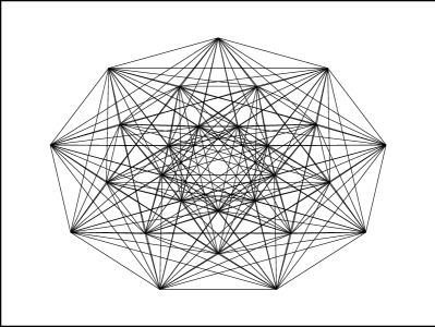
Figure 2: The Hessian polyhedron

and the vertices of a complex polytope of type $3\{3\}3\{4\}2$ (see Fig. 3).

Figure 3: The polyhedron $3\{3\}3\{4\}2$

In the case where $b=0$, we have to distinguish between the cases $c\not=0$ and $c=0$. If $c\not=0$, we find 648 triples, whatever the value of $a$. If $c=0$, we obtain 27 triples if $a\not=0$, and only one if $a=0$.

Indeed, for $b=c=0$, the $\psi$-equation reduces to $\psi^{8}=0$, and all the cubics collapse to $12U^{3}-aU=0$. For $a\not=0$ we obtain precisely 27 triples $(u,v,w)$ which form the vertices of a Hessian polyhedron in ${\mathbb{C}\,}^{3}$ (see Ref. Coxeter (1940)).

From the results of Ref. Orlik and Solomon (1982) about the arrangement of 12 planes formed by the mirrors of the pseudoreflections of $K=G_{25}$, we can determine the structure of the stabilizers of the normal forms. The only nontrivial cases are:

• the orbits with 216 elements, for which the stabilizer is the cyclic group $C_{3}$;

• the orbits with $72$ elements, for which it is $C_{3}\times C_{3}$;

• the Hessian orbits with 27 elements, for which it is the group $G_{4}$ of the Shephard-Todd classification.

These results can be regarded as a complete description of the moduli space of three qutrits states. To see what this means, let us recall some definitions from geometric invariant theory.

It is well known that it in general, the orbits of a group action on an algebraic variety cannot be regarded as the points of an algebraic variety. To remedy this situation, one has to discard certain degenerate orbits. It is then possible to construct a categorical quotient and a moduli space, which describe the geometry of sufficiently generic orbits, respectively in the affine and projective situation.

The categorical quotient $Y={\cal H}//G$ is defined as the affine variety whose affine coordinate ring is the ring of polynomial invariants $R={\mathbb{C}\,}[{\cal H}]^{G}$. The moduli space is the projective variety ${\cal M}={\rm Proj\,}(R)$ of which $R$ is the homogeneous coordinate ring. It is the quotient of the set ${\mathbb{P}}({\cal H})^{\rm ss}$ of semi-stable points by the action of $G$ (by definition, a point is semi-stable iff at least one of its algebraic invariants is nonzero, see Vinberg and Popov (1994)).

Now, since in our case the algebra of invariants is a polynomial algebra, we see that the categorical quotient is just the affine space ${\mathbb{C}\,}^{3}$.

The moduli space is more interesting. The projective variety whose homogeneous coordinate ring is a polynomial algebra over generators of respective degrees $d_{1},\ldots,d_{m}$ is called a weighted projective space ${\mathbb{P}}(d_{1},\ldots,d_{m})$. Hence, by definition, our moduli space ${\cal M}$ is the weighted projective space ${\mathbb{P}}(6,9,12)\simeq{\mathbb{P}}(2,3,4)$. It is known that this space is isomorphic to ${\mathbb{P}}(1,2,3)$ Dolgachev (1982), which in turn can be embedded as a sextic surface in ${\mathbb{P}}^{6}$, the so-called del Pezzo surface $F^{6}$ (see Ref. Harris (1992)). The del Pezzo surfaces are very interesting objects, known to be related to the exceptional root systems (see, e.g., Ref. Manin (1986)).

The above results can then be interpreted as a description of the singularities of ${\cal M}$, since one can view it as the quotient of the projective plane ${\mathbb{P}}^{2}$ of the parameters $(u:v:w)$ under the projective action of $G_{25}$. We have described this quotient as a 648-fold ramified covering ${\mathbb{P}}^{2}\rightarrow{\cal M}$, and analyzed its ramification locus.

VIII Conclusion

A problem of current interest in Quantum Information Theory has been connected to various important mathematical works, scattered on a period of more than one century from Ref. Maschke (1889) in 1889 to Ref. Nurmiev (2000a) in 2000, in general independent of each other and apparently discussing different subjects. Relying on all these works, we have described the geometry of the normal forms of semi-stable orbits of three qutrit states under the action of $SL(3,{\mathbb{C}\,})^{\times 3}$, the group of local filtering (SLOCC) operations. From a physical point a view, our results can be expected to provide a good starting point for studying the richness of the entanglement of three qutrits and its differences with that of the simpler qubit systems. From a mathematical point a view, we have worked out an interesting example of a problem in invariant theory, using both classical algebraic and modern geometric methods, found a surprising connection with the geometry of complex polytopes, and applied Klein’s vision of Galois theory to the explicit solution of an algebraic equation of degree 648.

Also, this example provides a good illustration of the ideas presented in Refs. Verstraete et al. (2001) and Klyachko (2002).

References

- Acín et al. [2000] Acín, A., A. Andrianov, L. Costa, E. Jané, J. I. Latorre, and R. Tarrach, 2000, Phys. Rev. Lett. 85, 1560.
- Bennett and Brassard [1984] Bennett, C., and G. Brassard, 1984, Proc. of the IEEE Int. Conf. on Computers, Systems and Signal Processing , 175.
- Briand et al. [2003] Briand, E., J.-G. Luque, and J.-Y. Thibon, 2003, J. Phys. A: Math. Gen. 36, 9915.
- Carteret et al. [2000] Carteret, H., A. Higuchi, and A. Sudbery, 2000, J. Math. Phys. 41, 7932.
- Chanler [1939] Chanler, J. H., 1939, Duke Math. J. 5, 552.
- Coolidge [1931] Coolidge, J. L., 1931, A treatise on algebraic plane curves (Oxford University Press (Clarendon), London).
- Coxeter [1940] Coxeter, H. S. M., 1940, Amer. J. Math. 62, 457.
- Coxeter [1991] Coxeter, H. S. M., 1991, Regular complex polytopes (Cambridge University Press, Cambridge), second edition.
- Dolgachev [1982] Dolgachev, I., 1982, in Group actions and vector fields (Vancouver, B.C., 1981) (Springer, Berlin), volume 956 of Lecture Notes in Math., pp. 34–71.
- Dür et al. [2000] Dür, W., G. Vidal, and J. Cirac, 2000, Phys. Rev. A 62, 062314.
- Ekert [1991] Ekert, A., 1991, Phys. Rev. Lett. 67, 661.
- Fitzi et al. [2001] Fitzi, M., N. Gisin, and U. Maurer, 2001, Phys. Rev. Lett. 87, 217901.
- Gelfand et al. [1994] Gelfand, I., M. Kapranov, and A. Zelevinsky, 1994, Discriminants, Resultants, and Multidimensional Determinants (Birkhäuser, Boston).
- Harris [1992] Harris, J., 1992, Algebraic geometry, a first course (Springer-Verlag, Berlin).
- Kaszlikowski et al. [2002] Kaszlikowski, D., D. Gosal, E. J. Ling, L. C. Kwek, M. Ukowski, and C. H. Oh, 2002, Phys. Rev. A 66, 032103.
- Klein [1884] Klein, F., 1884, Vorlesungen über das Ikosaeder und die Auflösung der Gleichungen vom fünften Grade (Teubner, Leipzig).
- Klyachko [2002] Klyachko, A. A., 2002, Coherent states, entanglement, and geometric invariant theory, quant-ph/0206012.
- Lamport et al. [1982] Lamport, L., R. Shostak, and M. Pease, 1982, ACM Trans. Programming Languages Syst. 4, 382.
- Luque and Thibon [2003] Luque, J.-G., and J.-Y. Thibon, 2003, Phys. Rev. A 67, 042303.
- Manin [1986] Manin, Y. I., 1986, Cubic forms, volume 4 of North-Holland Mathematical Library (North-Holland Publishing Co., Amsterdam), second edition.
- Maschke [1889] Maschke, H., 1889, Math. Ann. 33, 317.
- Miyake [2003] Miyake, A., 2003, Phys. Rev. A 67, 012108.
- Nurmiev [2000a] Nurmiev, A. G., 2000a, Uspekhi Mat. Nauk 55(2(332)), 143.
- Nurmiev [2000b] Nurmiev, A. G., 2000b, Mat. Sb. 191(5), 101.
- Olver [1999] Olver, P., 1999, Classical Invariant Theory (Cambridge University Press, Cambridge).
- Orlik and Solomon [1982] Orlik, P., and L. Solomon, 1982, Math. Ann. 261, 339.
- Shephard and Todd [1954] Shephard, G. C., and J. A. Todd, 1954, Canad. J. Math. 6, 274.
- Thrall [1938] Thrall, R. M., 1938, Amer. J. Math. 40, 383.
- Thrall and Chanler [1938] Thrall, R. M., and J. Chanler, 1938, Duke Math. J. 4, 678.
- Turnbull [1960] Turnbull, H. W., 1960, The theory of determinants, matrices and invariants (Dover, New York).
- Verstraete et al. [2002] Verstraete, F., J. Dehaene, B. De Moor, and H. Verschelde, 2002, Phys. Rev. A 65, 052112.
- Verstraete et al. [2001] Verstraete, F., J. Dehaene, and B. D. Moor, 2003, Phys. Rev. A 68, 012103.
- Vinberg [1975] Vinberg, È. B., 1975, Dokl. Akad. Nauk SSSR 221(4), 767.
- Vinberg [1976] Vinberg, È. B., 1976, Izv. Akad. Nauk SSSR Ser. Mat. 40(3), 488.
- Vinberg and Popov [1994] Vinberg, E. B., and V. L. Popov, 1994, in Algebraic geometry. IV, edited by I. R. Shafarevich (Springer-Verlag, Berlin), volume 55 of Encyclopaedia of Mathematical Sciences, pp. vi+284.
- Vollbrecht and Werner [2001] Vollbrecht, K., and R. Werner, 2001, Phys. Rev. A 64, 062307.
- Werner and Holevo [2002] Werner, R., and A. Holevo, 2002, Counterexample to an additivity conjecture for output purity of quantum channels, quant-ph/0203003.