Entangling quantum measurement and its properties

Abstract

We study the mathematical structure of superoperators describing quantum measurements, including the entangling measurement—the generalization of the standard quantum measurement that results in entanglement between the measurable system and apparatus. It is shown that the coherent information can be effectively used for the analysis of such entangling measurements whose possible applications are discussed as well.

I Introduction

Experiments in the field of quantum information processing and engineering, a new emerging interdisciplinary field of science QC , require the acquisition of information about the quantum system ($A$, hereafter, the “object”) by means of an apparatus that produces a measurement Neumann55 ; zurek ; Ludwig . During the measurement, the object quantum system and apparatus interact with each other (and with the environment or the “reference” system). As a result, the apparatus acquires essentially quantum information initially contained in the measurable quantum system.

The measurement procedure and the structure of the related measurement transformation may vary essentially. For example, in quantum optics the coherent measurement transformation is used gisin01 ; cohmeas . In applications to the emerging field of quantum information processing and quantum computing, quantum measurement can also be considered as an effective tool for realizing quantum algorithms childs02 . Although quantum measurement procedures can vary significantly for different applications it is worth selecting and examining mathematical forms of common types of measurement, their properties, and areas of possible applications.

In this work, we examine a class of quantum measurements completely preserving the initial concept of quantum measurement as the wave function collapse, $\psi\to\{p_{n}=|c_{n}|^{2},\mathop{\left|n\right\rangle}\nolimits\}$ sudbery ; Measur , i.e., the transfer of an initially pure state into a mixed ensemble of pure orthogonal states $\mathop{\left|n\right\rangle}\nolimits$ with probabilities $p_{n}$. We call such a measurement a standard measurement. The initial coherency in the object system (in the initial wave function $\psi=\sum c_{n}\mathop{\left|n\right\rangle}\nolimits$ between the eigenstates of the measurable variable $\hat{A}=\sum\lambda_{n}\mathop{\left|n\right\rangle}\nolimits\mathop{\left\langle n\right|}\nolimits$) is therefore completely lost. Since it happens for any quantum state $\psi$, this means that the object quantum system is completely dequantized, i.e., the only subset of orthogonal states $\mathop{\left|n\right\rangle}\nolimits$ out of all the system states $\psi$ is left. This subset is equivalent to a set of classical events. The final states of the apparatus can then be characterized by a measurable variable $\hat{M}$, which we will call a “pointer” preskill . After the measurement, the pointer has the same values as those of $\hat{A}$.

The generalization of this concept discussed here lies in considering a more general set of states after the quantum measurement, which takes into account the created entanglement in the object–pointer system after the measurement. We will call such a measurement an entangling measurement. Note that the entangling measurement introduced here is qualitatively different from the measurement transformation defined in Ref. vedral02, , where it is introduced in the form of a unitary transformation, and from the transformation defined in Refs. ozawa01, ; barnum02, , where the quantum properties of states in the bipartite system object–pointer are not considered. Also, it is worth noting that the measurement transformations in the bipartite system are clearly related to the characterization of transformations in the bipartite setting Alice–Bob restricted by physical causality relations Preskill-pap .

One of the fundamental properties of a measurement transformation is that the resulting state of the bipartite system object–pointer does not depend on the initial state of the apparatus. In case of an entangling measurement, this property, which makes the transformation irreversible, distinguishes it from reversible transformations of quantum entanglement, which play a fundamental role in quantum information processing QC and can be realized with the help of a unitary transformation applied to the bipartite system.

In quantum information theory, entanglement is one of the key concepts used for characterization of quantum states of a bipartite setting. It determines the quantum specifics of physical interaction on which such its practical applications as quantum computing and quantum cryptography rely QC ; UFN01 . For a bipartite system object–pointer in a pure state described by a joint wave function $\psi_{AM}$, there is a unique definition of the degree of quantum entanglement as the entropy of separate density matrices $S(\hat{\rho}^{A})=S(\hat{\rho}^{M})$, where $\hat{\rho}^{A}={\rm Tr}_{M}\psi_{AM}\psi_{AM}^{+}$ and $\hat{\rho}^{M}={\rm Tr}_{A}\psi_{AM}\psi_{AM}^{+}$. However, for the case of mixed states there is no unique valid definition of the degree of entanglement.

In this connection, it is worth noting that the entanglement of quantum states created here is due to the above-specified alternative choice of the quantum measurement procedure. One can even assume that the characterization of the degree of entanglement as a derivative from the transformation measurement structure realized by an apparatus can give some additional information about the physical contents of the entanglement concept.

In Sec. II, we give precise mathematical definitions of both standard and entangling measurement transformations, special cases of which are considered in Sec. III. We describe the general structure of a quantum measurement superoperator and specify structure of the entanglement matrix and the entangling measurement superoperator in Sec. IV. The discussed formalism is clarified by an example of a two-dimensional model. In Sec. V we address the question whether an entangling measurement can be used for an entanglement transfer in various applications of quantum information processing. We prove that it cannot be used for the entanglement transfer from a bipartite system to another one. We consider the quantitative characteristics of entanglement in Sec. VI arguing that the coherent information is a valid tool for characterizing the entanglement created in the bipartite system object–pointer.

II Mathematical definitions of quantum measurement transformations

Following the traditional quantum measurement postulate Neumann55 ; zurek ; Ludwig ; Measur , the process of quantum measurement of a quantum object system $A$ that lives in Hilbert space $H_{A}$ by the classical pointer variable $M$ leads to establishing the resulting state of the system $A$. In this state the measurable physical variable described by a quantum operator $\hat{A}$ takes one of the range of possible values $\lambda$ and the apparatus’ classical variable $M$ coincides with that value: $M=\lambda$. We then can simplify the description of the apparatus preserving only the initial ($\mu$) and resulting ($\lambda$) values of the pointer variable. After this simplification, the measurement transformation in the bipartite system “quantum object–pointer” is represented by the superoperator quantum transformation along the quantum variables of the measurable system $A$ and the classical conditional probability distribution along the classical pointer variables $\mu$ of the apparatus QSP :

$${\cal M}(\lambda|\mu)=\hat{P}_{\lambda}^{A}\odot\hat{P}_{\lambda}^{A}.$$ (1)

A symbolic representation of the quantum state transformation operators is used here, in which the substitution symbol $\odot$ is to be substituted by a transformed operator. The operators $\hat{P}_{\lambda}^{A}$ are the orthogonal projectors onto the subspaces with eigenvalue $\lambda$ of the measurable variable $\hat{A}=\sum\lambda\hat{P}_{\lambda}^{A}$, where $\lambda$ enumerates the final states of the apparatus (there is no dependence on $\mu$, which indicates independence from the initial state of the pointer).

The initial states of the bipartite system “quantum object system–apparatus” are described by the joint quantum-classical distributions $\hat{\rho}(\mu)$ defined as the linear operators in the direct product $H_{A}\otimes\Lambda_{M}$ of the Hilbert space of the quantum system and the set $\Lambda_{M}$ of classical values of the pointer variable. They obey the positivity requirement $\hat{\rho}(\mu)\geq 0$ (i.e., $\mathop{\left\langle\psi\right|}\nolimits\hat{\rho}(\mu)\mathop{\left|\psi\right\rangle}\nolimits\geqq 0$ for any $\psi$ and all $\mu$) and the normalization condition $\sum_{\mu}{\rm Tr}\,\hat{\rho}(\mu)=1$ and are transformed with the help of the superoperator (1) as

$$\hat{\rho}(\mu)\to\hat{\rho}(\lambda)=\sum_{\mu}{\cal M}(\lambda|\mu)\hat{\rho}(\mu)=\sum_{\mu}\hat{P}_{\lambda}^{A}\hat{\rho}(\mu)\hat{P}_{\lambda}^{A}.$$ (2)

Here we restrict our consideration to the class of “direct” measurements that are described by the orthogonal projectors $\hat{P}_{\lambda}^{A}$, having in mind the fundamental character of this subclass of all possible measurements. More general measurements can then be smoothly handled in the open systems framework.

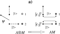
Figure 1: Special cases of a quantum measurement. a) Standard measurement in the bipartite setting “quantum object–classical pointer”: the wave function $\psi$ and independent state “2” of the classical apparatus transfer into the statistical mixture of totally-correlated states $\mathop{\left|i\right\rangle}\nolimits\otimes\,i$ of the bipartite system $AM$ with probabilities $|c_{i}|^{2}$ $(i=1,2)$. b) An entangling measurement in the bipartite setting “quantum object–quantum pointer” for the entanglement matrix $R_{ij}\equiv 1$ (Sec. III): an independent pure state of the bipartite system transfers into an entangled state, which is the coherent superposition $c_{1}\mathop{\left|1\right\rangle}\nolimits\mathop{\left|1\right\rangle}\nolimits+c_{2}\mathop{\left|2\right\rangle}\nolimits\mathop{\left|2\right\rangle}\nolimits$.

The linear transformation discussed above is defined on the direct product ${\mathbb{C}}_{AM}={\mathbb{C}}(H_{A})\otimes{\mathbb{C}}(\Lambda_{M})$ of the quantum-mechanical operator algebra in $H_{A}$ and the algebra of classical functions on the set $\Lambda_{M}$. This transformation yields the pointer value $\lambda$ (independent of its initial values $\mu$) for the density matrices of the pure state $\hat{\rho}^{A}_{\lambda}=\psi\psi^{+}$ with wave functions $\psi$ of the measurable quantum system, which lie in the eigen subspaces $\Phi_{\lambda}$ corresponding to the value $\lambda$ of the measurable variable, i.e., $\hat{P}_{\lambda}^{A}\psi=\psi\in\Phi_{\lambda}$. If the measurement is a complete one, i.e., $\Phi_{\lambda}$ are one-dimensional, then the transformation (2) for an arbitrary density matrix $\hat{\rho}^{A}$ in a joint initial state of the form $\hat{\rho}(\mu)=\hat{\rho}^{A}\otimes p(\mu)$ describes the output mixture of the corresponding pure states $\hat{P}_{\lambda}^{A}=\mathop{\left|\lambda\right\rangle}\nolimits\mathop{\left\langle\lambda\right|}\nolimits$ with probability weights $p(\lambda)=\mathop{\left\langle\lambda\right|}\nolimits\hat{\rho}\mathop{\left|\lambda\right\rangle}\nolimits$. A scheme clarifying the measurement transformation structure in the described quantum-classical system is shown in Fig. 1 .

The problem of the physical realizability of a quantum system measurement procedure with the help of a classical system has attracted considerable interest in the literature, but some principal questions related to this problem are still under discussion Peres ; Marsh ; Zhang ; Sokol . A simple example clarifying the key mechanisms for realizing the measurement procedure (1) in a closed physical system described quantum-mechanically to preserve the quasiclassical character of the apparatus’ variable, is given in Ref. QSP, .

Along with the maximally simplified description of the measurement procedure in the form of superoperator (1), which takes into account the physical structure of the apparatus only in the form of the classical variable $\mu\to\lambda$, a more detailed description must at least include the quantum-mechanical variables of the apparatus that are complimentary to the classical variable. In this case, a minimal extension of the model leads to the replacement of the classical apparatus’ pointer with a quantum one, which lives in the space $H_{M}$ with dimension $D$ equal to the number of values of the measurable variable.

Accordingly, superoperator (1) is replaced with the fully quantum superoperator of the standard measurement

$${\cal M}_{AM}=\sum\limits_{\lambda}\bigl{(}\hat{P}_{\lambda}^{M}{\rm Tr}_{M}\odot\bigr{)}\otimes\bigl{(}\hat{P}_{\lambda}^{A}\odot\hat{P}_{\lambda}^{A}\bigr{)}.$$ (3)

Here the $\hat{P}_{\lambda}^{A}$ are the same as in Eq. (1) and the $\hat{P}_{\lambda}^{M}$ are the one-dimensional projectors corresponding to the values $\lambda$ of the apparatus’ variable $\hat{M}=\sum\lambda\hat{P}^{M}_{\lambda}$.

Projecting the density matrix of the measurable quantum system described by the operators $\hat{P}_{\lambda}^{A}$ leads to the transformation of the system’s state into an incoherent superposition of respected states with explicitly determined values $\lambda$ of the variable $\hat{A}$. Operation ${\rm Tr}_{M}\odot$ reflects the independence of the final state of the apparatus from its initial state and the projectors $\hat{P}^{M}_{\lambda}$ describing the resulting quantum state of the pointer after the measurement, which correspond to the measured values $\lambda$. In the general case, the projectors $\hat{P}_{\lambda}^{M}$ considered in the real physical space of the apparatus are multidimensional; this corresponds to macroscopic systems with numerous internal degrees of freedom of the apparatus. However, if these internal degrees of freedom do not affect essentially the interaction of the apparatus with the measurable quantum system, the measurement can be adequately described in the minimal Hilbert space $H_{M}$.

Superoperator (3), being physically realizable, is completely positive kraus and, additionally, is hermitian with respect to the scalar product $(\hat{\rho}_{1},\hat{\rho}_{2})={\rm Tr}\,\hat{\rho}_{1}^{+}\hat{\rho}_{2}$. Then, its particular property of idempotency, i.e., ${\cal M}_{AM}^{2}={\cal M}_{AM}$, identifies an orthogonal projector onto the subspace of unperturbed states of the bipartite system “object–pointer”.

In the description of the measurement procedure given above, the quantum nature of the apparatus is not essential, though it is virtually present in its mathematical description. Only the pointer variable is used and the off-diagonal quantum operators are simply not considered. Mathematically, it means that we consider a reduced algebra of quantum events ${\mathbb{B}}$ of the quantum probabilistic space $(H,{\mathbb{B}},{\cal P})$, where $H$ is the Hilbert space of all states allowed in the quantum system, $\mathbb{B}$ is the algebra of its subspaces $\Omega\subseteq H$ identified by the orthoprojectors $\hat{P}(\Omega)$, and ${\cal P}(\Omega)={\rm Tr}\,\hat{P}(\Omega)\hat{\rho}$ is the quantum probability distribution defined with the help of the density matrix. In this quasiclassical case, the algebra of orthogonal subspaces in $H_{M}$ built on the eigen subspaces $\Phi_{\lambda}$ of the eigen projectors $\hat{P}_{\lambda}^{M}$ of the apparatus’ variable $\hat{M}$ is used for the description of the pointer variable ${\mathbb{B}}$. However, besides the variables commuting with the pointer variable $\hat{M}$ there are also off-diagonal variables of the form $\hat{N}=\sum_{\lambda\mu}N_{\lambda\mu}\mathop{\left|\lambda\right\rangle}\nolimits^{M}\mathop{\left\langle\mu\right|}\nolimits^{M}$ that do not commute with $\hat{M}$ and can potentially lead to the essentially quantum nature of the apparatus even at macroscopic level.

The fact that in a real macroscopic system there exist variables, which do not commute with $\hat{P}_{\lambda}^{M}$, is not a paradox. In physics, pithy examples of such quantum variables in quasiclassical systems arise, for instance, when considering polyatomic molecules (an effective two-level model of molecular chirality related to the chiral degree of freedom of a chiral molecule having stable enantiomers can serve as such a pithy example bychkov ; JRS02 ). Similar subsystems can be extracted in the mathematical description of a complete set of potentially possible states of any macroscopic system. Typically, their quantum nature is not essential because of the small values of energy quanta corresponding to the transitions between discrete energy levels.

On the contrary, there is also a number of macroscopical quantum systems, i.e., quantum dots, superconducting Josephson junctions, and others, which are considered as embodies of qubits in quantum information processing QC where the quantum nature of the apparatus can be essential. Specific models of apparatus can, obviously, limit both the quality and fidelity of reproduction of the measurement transformation (3) due to the macroscopic nature of the apparatus. However, as follows from the analysis of numerous specific models in the literature, such limitations do not forbid realizations of such measurement models.

An initial density matrix of the form $\hat{\rho}^{A}{\otimes}\hat{\rho}^{M}$ is transformed by the superoperator (3) into the density matrix

$$\hat{\rho}^{AM}=\sum\limits_{\lambda}\bigl{(}\hat{P}_{\lambda}^{A}\hat{\rho}^{A}\hat{P}_{\lambda}^{A}\bigr{)}\otimes\hat{P}_{\lambda}^{M}$$ (4)

characterizing the state with the coinciding variables “$\hat{A}{=}\hat{M}$”, i.e., in strict form $(\hat{A}-\hat{M})\hat{\rho}^{AM}=0$. This state is an incoherent statistical mixture of quantum states characterizing each of the variables. The transfer of information between the quantum system $A$ and apparatus $M$ is realized in such a state through the classical variable $\lambda$. Quantum fluctuations therefore exist only virtually as uncertainty in the physical variables, which do not commute with $\hat{A}$ and $\hat{M}$ and are therefore not determined explicitly.

The above-described semiclassical concept of the measurement is not a general one Neumann55 ; Ludwig ; Stenholm . Moreover, generation of entanglement by means of quantum measurement has been a topical issue for the last decade Kuzmich ; Duan ; Kozhekin ; Molmer ; Jakob . Therefore, a generalization of the standard measurement approach can essentially extend the concept of quantum measurement.

For example, an essentially quantum isometric (at fixed $\psi_{M}$) transformation $\psi_{A}\otimes\psi_{M}\to\sum{\mathop{\left\langle k\left|\psi_{A}\right.\right\rangle}\nolimits}_{A}{\mathop{\left|k\right\rangle}\nolimits}_{A}{\mathop{\left|k\right\rangle}\nolimits}_{M}$ of an arbitrary pure state into an entangled state can be interpreted as a measurement of the variable $\hat{A}=\sum\lambda_{k}{\mathop{\left|k\right\rangle}\nolimits}_{A}{\mathop{\left\langle k\right|}\nolimits}_{A}$ with the help of the apparatus’ variable $\hat{M}=\sum\lambda_{k}{\mathop{\left|k\right\rangle}\nolimits}_{M}{\mathop{\left\langle k\right|}\nolimits}_{M}$. The corresponding generalization of the measurement superoperator (3) has the form

$${\cal M}_{0}=\sum\limits_{kl}\bigl{(}\hat{P}_{kl}^{M}{\rm Tr}_{M}\odot\bigr{)}\otimes\bigl{(}\hat{P}_{kk}^{A}\odot\hat{P}_{ll}^{A}\bigr{)},$$ (5)

where the $\hat{P}_{kl}=\mathop{\left|k\right\rangle}\nolimits\mathop{\left\langle l\right|}\nolimits$ are the one-dimensional projectors from $\mathop{\left|l\right\rangle}\nolimits$ onto $\mathop{\left|k\right\rangle}\nolimits$ in the respective Hilbert spaces $H_{A}$ and $H_{M}$. For a pure state $\hat{\rho}^{A}=\mathop{\left|\psi_{A}\right\rangle}\nolimits\mathop{\left\langle\psi_{A}\right|}\nolimits$, this transformation ensures the resulting pure entangled state of the composite system. Note, however, that this does not mean the absence of dequantization of the initial state, because the latter is represented in the final state only by the diagonal orthoprojectors $\hat{P}_{kk}^{A}$ and $\hat{P}_{ll}^{A}$.

The above formulas for the measurement superoperators ${\cal M}_{AM}$ and ${\cal M}_{0}$ can be generalized to an intermediate representation of the form

$${\cal M}=\sum\limits_{kl}R_{kl}\bigl{(}\hat{P}_{kl}^{M}{\rm Tr}_{M}\odot\bigr{)}\otimes\bigl{(}\hat{P}_{kk}^{A}\odot\hat{P}_{ll}^{A}\bigr{)},$$ (6)

which describes an entangling measurement with the Hermitian entanglement matrix $R_{kl}$. This matrix is chosen to ensure the complete positivity and normalization condition for the measurement transformation. To our knowledge, Eq. (6) is the most general form of the entangling measurement superoperator based on the linear combination of the input-output projectors, which is compatible with the ideal measurements concept.

At $R_{kl}=\delta_{kl}$, Eq. (6) simplifies to the standard quantum measurement (3), if one identifies the projector sets with corresponding indices $k$ and $\lambda$. The projectors $\hat{P}^{A}_{kk}$ in Eq. (6) characterize information in the quantum system to be measured and its statistical properties are determined by the density matrix $\hat{\rho}^{A}$. Information that is finally measured by the apparatus is represented by the projectors $\hat{P}^{M}_{kl}$, and its statistical properties are determined only by the density matrix $\hat{\rho}^{A}$ and are invariant with respect to the choice of a basis in the state space $H_{M}$ of the apparatus.

The measurement transformation (6) creates an entanglement in the bipartite system “quantum object system–apparatus” whose value may vary between zero and its maximum value (which depends on $R_{kl}$).

Taking the basis set of the density matrices in the form $\hat{\rho}^{A}{\otimes}\hat{\rho}^{M}$, we obtain for the transformation of the joint density matrix:

$$\hat{\rho}^{AM}={\cal M}\,\hat{\rho}^{A}\otimes\hat{\rho}^{M}=\sum R_{kl}\rho^{A}_{kl}\hat{P}_{kl}^{A}\otimes\hat{P}_{kl}^{M}.$$ (7)

For the initial density matrix of the composite system of general form $\hat{\rho}^{AB}$, the resulting matrix has the same form (7), keeping in mind that the matrix elements $\rho^{A}_{kl}$ correspond to the partial density matrix $\hat{\rho}^{A}={\rm Tr}_{B}\hat{\rho}^{AB}$. Therefore, the density matrix of a composite system is formed in the process of measurement as a result of the dubbing ${\mathop{\left|k\right\rangle}\nolimits}^{A}\to\mathop{\left|k\right\rangle}\nolimits^{A}\mathop{\left|k\right\rangle}\nolimits^{A}$ of the chosen object basis, accompanied by multiplication of the corresponding elements of the initial density matrix of the object by those of the entanglement matrix.

III Special cases

Let us assume that the initial state of a quantum system is a pure state, i.e., $\hat{\rho}^{A}=\psi_{A}\psi^{+}_{A}$ with $\psi_{A}=(c_{1},\dots,c_{D})$, and the measurement procedure is complete, which means that all the projectors $\hat{P}_{kl}$ are one-dimensional. Then, it follows from Eq. (7) that

$$\hat{\rho}^{AM}=\sum\limits_{k}\varkappa_{k}\mathop{\left|\mathop{\left|k\right\rangle}\nolimits\right\rangle}\nolimits\mathop{\left\langle\mathop{\left\langle k\right|}\nolimits\right|}\nolimits,\quad\mathop{\left|\mathop{\left|k\right\rangle}\nolimits\right\rangle}\nolimits=\sum\limits_{i}e_{ki}\mathop{\left|i\right\rangle}\nolimits\mathop{\left|i\right\rangle}\nolimits,$$ (8)

where the $\varkappa_{k}$, $e_{k}=(e_{k1},\dots,e_{kD})$ are the eigenvalues and the respective normalized eigenvectors of the matrix $\tilde{\rho}_{kl}=R_{kl}\rho_{kl}=R_{kl}c_{k}c^{*}_{l}$. This means that the pure state is transformed into an incoherent mixture of pure entangled states of the bipartite system “object–pointer”, which are orthogonal to each other and have different degrees of entanglement that depends on the entanglement and density matrices. For the case of $\hat{\rho}^{A}=\mathop{\left|k_{0}\right\rangle}\nolimits\mathop{\left\langle k_{0}\right|}\nolimits$, we have $c_{k}=\delta_{kk_{0}}$ and the corresponding joint density matrix $\hat{\rho}^{AM}=\mathop{\left|k_{0}\right\rangle}\nolimits^{A}\mathop{\left\langle k_{0}\right|}\nolimits^{A}\otimes\mathop{\left|k_{0}\right\rangle}\nolimits^{M}\mathop{\left\langle k_{0}\right|}\nolimits^{M}$, which coincides with the density matrix resulting from the standard measurement ${\cal M}_{AM}$ of the observable $\hat{A}=\sum\lambda_{k}\mathop{\left|k\right\rangle}\nolimits^{A}\mathop{\left\langle k\right|}\nolimits^{A}$. For the case of pure maximum uncertainty state $\hat{\rho}^{A}=(1/D)\sum\mathop{\left|k\right\rangle}\nolimits\mathop{\left\langle k\right|}\nolimits$, we have $\hat{\rho}^{AM}=\sum_{kl}(R_{kl}/D)\mathop{\left|\mathop{\left|k\right\rangle}\nolimits\right\rangle}\nolimits\mathop{\left\langle\mathop{\left\langle l\right|}\nolimits\right|}\nolimits$ with $\mathop{\left|\mathop{\left|k\right\rangle}\nolimits\right\rangle}\nolimits=\mathop{\left|k\right\rangle}\nolimits\mathop{\left|k\right\rangle}\nolimits$, where $R_{kl}/D$ is the object–pointer density matrix in the basis of the dubbed (“cloned”) states.

For the entanglement matrix $R_{ij}=\delta_{ij}$, all the eigenvalues $\varkappa_{k}=|c_{k}|^{2}$ in Eq. (8) are represented by the eigenvectors $e_{ki}=\delta_{ki}$ and the degree of entanglement of each of the $\mathop{\left|\mathop{\left|k\right\rangle}\nolimits\right\rangle}\nolimits$ states is equal to zero. Thus, a completely incoherent mixture of states of the measurable variable $\hat{A}=\sum\lambda_{i}\mathop{\left|i\right\rangle}\nolimits\mathop{\left\langle i\right|}\nolimits$ with determined $\lambda_{i}$ is formed.

For the entanglement matrix $R_{ij}\equiv 1$, which has the only nonzero eigenvalue $\varkappa_{k}=1$ and respective eigenvector $e_{ki}=c_{i}$, Eq. (8) gives us a pure state, which is represented by the single vector

$$\mathop{\left|\mathop{\left|k\right\rangle}\nolimits\right\rangle}\nolimits=\sum c_{i}\mathop{\left|i\right\rangle}\nolimits\mathop{\left|i\right\rangle}\nolimits.$$

The state $\mathop{\left|\mathop{\left|k\right\rangle}\nolimits\right\rangle}\nolimits=\sum c_{i}\mathop{\left|i\right\rangle}\nolimits\mathop{\left|i\right\rangle}\nolimits$, corresponding to the state in Eq. (8), coincides with the state formed after the quantum duplication transformation PRA00 . The degree of its entanglement $E$ can be estimated as the entropy $S[P]$ of the probability distribution $P(i)=|c_{i}|^{2}$ of all possible values $\lambda_{i}$ of the measurable variable. We can always receive a maximum possible degree of entanglement $E=\log_{2}D$ by choosing the measurable variable $\hat{A}$ as having maximum uncertainty in the state $\psi$, which corresponds to the vector representation $c_{i}\equiv 1/\sqrt{D}$ and the uniform distribution $\psi\to P(i)=1/D$. Therefore, for the maximally entangling measurement, vacuum quantum fluctuations of the measurable variable are transferred into the corresponding entanglement of the bipartite system “object–pointer”.

For the general case of a mixed initial state $\hat{\rho}^{A}=\sum\rho_{l}\mathop{\left|l\right\rangle}\nolimits\mathop{\left\langle l\right|}\nolimits$, an incoherent mixture of $D$ orthogonal (at fixed $l$) sets of entangled states $\mathop{\left|\mathop{\left|k,l\right\rangle}\nolimits\right\rangle}\nolimits$ is formed. These sets, however, are not necessarily orthogonal at different values of $l$, but this nonorthogonality is largely of formal character and physically does not mean nonorthogonality of the states of one and the same Hilbert spaces. When one considers an incoherent mixture of states, phase uncertainty is due to an additional degree of freedom, and incoherence means that we consider physically distinguishable (orthogonal RTE02 ; fuchs ) states. In fact, the orthogonal wave functions $\psi,\varphi$ correspond to two physically distinguishable states $i,j$ that describe different phases in the composite states $\psi=\mathop{\left|\alpha\right\rangle}\nolimits\mathop{\left|i\right\rangle}\nolimits$, $\varphi=\mathop{\left|\beta\right\rangle}\nolimits\mathop{\left|j\right\rangle}\nolimits$ even for nonorthogonal states $\alpha$ and $\beta$. Keeping this in mind, in a more detailed quantum description of a composite system, which includes all physically valuable degrees of freedom, quantum operators of the corresponding physical subsystems do commute.

IV General structure of the quantum measurement superoperator and analysis of a two-dimensional model

Let us first define the constraints imposed on the quantum measurement superoperator by the normalization condition and positivity property. From Eq. (7) we obtain ${\rm Tr}\,\hat{\rho}^{AM}=\sum R_{kk}\rho^{A}_{kk}$, which, with an arbitrary choice of $\hat{\rho}^{A}$, immediately gives the normalization condition $R_{kk}\equiv 1$. The positivity requirement and, simultaneously, the complete positivity properties require the positivity of the matrix $\hat{\rho}^{A}_{e}=\left(R_{kl}\rho^{A}_{kl}\right)$ for an arbitrary positive matrix $\hat{\rho}^{A}=\left(\rho^{A}_{kl}\right)$. Then, using the spectral representation of both these matrices, one can readily show that a necessary and sufficient condition for this requirement is the positivity of the entanglement matrix $R=\left(R_{kl}\right)$.

A repeated entangling measurement, i.e., the repeated application of the same measurement superoperator on the same apparatus–system Hilbert space, leads, on account of the measurement superoperator (6), equality $R_{kk}\equiv 1$, and vanishing of the off-diagonal elements of the pointer density matrix after tracing out ${\rm Tr}_{M}\odot$, to the relation

$${\cal M}^{2}={\cal M}_{AM}.$$ (9)

Therefore, a repeated entangling measurement leads to entanglement destruction and the resulting transformation is equal to the standard measurement. This entanglement destruction in the initial state of the “quantum object–pointer” is due to a “resetting” of the apparatus needed to achieve independence of the final system–apparatus state from the initial apparatus state.

Eq. (9) is valid for any entangling matrix $R$, i.e., the entangling measurement ${\cal M}$ is the ambiguous square root of the standard measurement ${\cal M}_{AM}$, which reveals in the spectrum structure of the corresponding matrices representing ${\cal M}$.

As an example, let us consider a two-level system with ${\rm dim}\,H_{A}=2$ for which the positivity criterion gives the following general form for the entanglement matrix:

$$R=\left({\begin{array}[]{cc}1&q\\ q^{*}&1\end{array}}\right),\quad|q|^{2}\leq 1.$$ (10)

The eigenvalue equation for the measurement superoperator

$${\cal M}\,\hat{\rho}^{AM}=\lambda\,\hat{\rho}^{AM}$$ (11)

can be solved analytically once we have expressed it in the form

$$\sum_{kl}\sum_{m}R_{kl}\rho^{AM}_{klmm}\hat{P}_{kl}^{A}\otimes\hat{P}_{kl}^{M}=\lambda\sum_{kl}\sum_{mn}\rho_{klmn}^{AM}\hat{P}_{kl}^{A}\otimes\hat{P}_{mn}^{M}\to R_{kl}\Bigl{(}\sum_{\mu}\rho^{AM}_{kl\mu\mu}\Bigr{)}\delta_{km}\delta_{ln}=\lambda\rho_{klmn}^{AM}.$$

For $D=2$, the dimension of the problem is limited to 16 possible values of the four-dimensional index $klmn$ of the “density matrix” (in the eigenvalue problem, in addition to physically valuable density matrices, arbitrary operators are considered, as well).

On account of the vanishing off-diagonal elements in the transformed density matrix $\rho^{AM}_{klmn}$ on the left-side of the above equation, we find that eight right eigen null-vectors $\hat{e}_{AM}^{0k}$, $k=1,\dots,8$ corresponding to the eigenvalue $\lambda=0$ are described by the following operators:

$$\hat{e}_{AM}^{0k}=\left\{\begin{array}[]{c}\!\hat{\rho}_{A}^{0k}\otimes\hat{P}_{12}^{M},\;k=1,2,3,4,\\ \hat{\rho}_{A}^{0k}\otimes\hat{P}_{21}^{M},\;k=5,6,7,8,\end{array}\right.$$ (12)

which have zero diagonal matrix elements $\rho^{AM}_{klmm}$ along $M$ with arbitrary density matrices $\hat{\rho}_{A}^{0k}$. Freedom in choosing them is due to the eightfold degeneracy and related to the arbitrary choice of four linearly independent basis vectors (12) corresponding to the related basis operators $\hat{P}_{12}^{M}$, $\hat{P}_{21}^{M}$ of the pointer $M$.

The other four zero eigenvectors satisfy the relation $\hat{\rho}_{kl11}^{AM}=-\hat{\rho}_{kl22}^{AM}$ and have the form

$$\hat{e}_{AM}^{0k}\,=\hat{\rho}_{A}^{0k}\otimes\bigl{(}\hat{P}_{22}^{M}-\hat{P}_{11}^{M}\bigr{)},\quad k=9,10,11,12$$ (13)

with arbitrary linearly independent density matrices $\hat{\rho}_{A}^{0k}$.

Finally, for two nonzero eigenvectors with $\lambda=1$ we have a pair of linearly independent functions $\rho_{k}=\delta_{k1},\delta_{k2}$ satisfying the relations $\rho^{1,k}_{klmn}=\rho_{k}\delta_{kl}\delta_{km}\delta_{ln}$ and corresponding operators

$$\hat{e}_{AM}^{1k}\,=\left\{\begin{array}[]{c}\hat{P}^{A}_{11}\otimes\hat{P}^{M}_{11}\\ \hat{P}^{A}_{22}\otimes\hat{P}^{M}_{22}\end{array}\right.,\quad k=13,14.$$ (14)

These two operators provide a basis of the convex set $p\,\hat{e}^{1,13}_{AM}+(1-p)\hat{e}^{1,14}_{AM}$ ($0\leq p\leq 1$) of the density matrices, which are not changed in the measurement transformation.

The last two linearly independent operators $\hat{e}^{015}_{AM}=\hat{P}^{A}_{12}\otimes\hat{I}^{M}$ and $\hat{e}^{016}_{AM}=\hat{P}^{A}_{21}\otimes\hat{I}^{M}$ are the eigen operators with eigenvalue equal to zero only at $R_{kl}=\delta_{kl}$ when the measurement is a standard measurement, not an entangling measurement. In the general case, the superoperator $\cal M$ lacks two eigenvectors, because it is not described by a matrix of simple structure similar to the single-mode fermion annihilation operator $\hat{a}=\left(\begin{array}[]{cc}0&1\\ 0&0\end{array}\right)$, which has a single non-vanishing right eigenvector $e_{0}=(1,0)$ note1 . Accordingly, Eq. (9) is realized as the relation $\hat{a}^{2}=0$, which washes out dependence of the squared operator on the entangling parameter $q$.

The corresponding linear subspace $c_{15}\hat{e}^{015}_{AM}+c_{16}\hat{e}^{016}_{AM}$ contains only density matrices, which have no physical meaning. Nevertheless, this subspace cannot be excluded from the complete 16D-space, because it is included into the cone of all positive hermitian density matrices.

The entangling measurement superoperator matrix in the “eigen” basis $\hat{e}_{AM}^{\lambda k}$ has the form:

$${\cal M}=\left(\begin{array}[]{ccccccc}1&0&\hat{\underline{0}}&0&0&0&0\\ 0&1&\hat{\underline{0}}&0&0&0&0\\ \hat{0}|&\hat{0}|&\hat{\rm O}&\hat{0}|&\hat{0}|&\hat{0}|&\hat{0}|\\ 0&0&\hat{\underline{0}}&0&0&q&0\\ 0&0&\hat{\underline{0}}&0&0&0&q^{*}\\ 0&0&\hat{\underline{0}}&0&0&0&0\\ 0&0&\hat{\underline{0}}&0&0&0&0\end{array}\right),$$ (15)

where $\hat{O}$ is a $10\times 10$ zero matrix, and $\hat{\underline{0}}$ and $\hat{0}|$ are 10-component zero bra- and ket-vectors, respectively. In the matrix (15), 4th and 5th lines correspond to the transversal–transversal basis operators and two bottom lines correspond to the two non-eigen operators $\hat{P}_{12}\otimes\hat{I}/D$, $\hat{P}_{21}\otimes\hat{I}/D$. The subspaces corresponding to the matrix (15) are 2D invariant, 12D zero, and 2D improper subspaces.

V Can entangling measurement be used for entanglement transfer?

In many applications of quantum information processing algorithms, such as practically interesting cryptographic protocols, require realization of a pair of spatially separated entangled quantum systems QC ; preskill . They serve as resources for quantum information engineering and developing technologies for their creation is of prime importance UFN01 . Deterministic creation of spatially separated entangled quantum systems is a difficult problem to solve. By contrast, pairs of entangled subsystems exist naturally and spontaneously within many spatially-localized physical systems.

For example, conservation of the total momentum of an atom is not related to the separate conservation of its components, orbital and spin momenta. Thus, the eigen states of the atom are, in the general case, entangled states related to subsystems describing orbital and spin momenta separately. Another example is laser excitation of ro-vibrational states in molecules, which results in the entanglement between the vibrational and rotational degrees of freedom.

Now, the following question arises, “Can these naturally entangled states be used for a transfer of their entanglement onto an entanglement of spatially separated quantum systems with the help of an entangling measurement?”.

To answer this question, let us consider four systems $A$, $B$, $M$, and $N$ with an initial state $\hat{\rho}^{ABMN}=\hat{\rho}^{AB}\otimes\hat{\rho}^{M}\otimes\hat{\rho}^{N}$. We assume that two of them, $A$ and $B$, are in the initially entangled state $\hat{\rho}^{AB}$, whereas systems $M$ and $N$ are initially independent and spatially separated from $A$, $B$. We will then check if it is possible to transfer entanglement from the bipartite system $A$–$B$ onto the bipartite system $M$–$N$ by applying two independent transformations ${\cal M}_{A}$ and ${\cal M}_{B}$ to the subsystems $A$–$M$ and $B$–$N$, respectively. The corresponding joint superoperator has the form

$${\cal M}_{B}\otimes{\cal M}_{A} = \sum\limits_{klmn}R_{kl}R_{mn}\bigl{[}\hat{P}^{B}_{mn}\otimes\bigl{(}\hat{P}^{N}_{mm}\odot\hat{P}^{N}_{nn}\bigr{)}{\rm Tr}_{B}\odot\bigr{]}$$

$$\otimes\bigl{[}\hat{P}^{A}_{kl}\otimes\bigl{(}\hat{P}^{M}_{kk}\odot\hat{P}^{M}_{ll}\bigr{)}{\rm Tr}_{A}\odot\bigr{]},$$

where systems $M$ and $N$ are treated as pointers for the measurements of systems $A$ and $B$. The resulting state of the bipartite system $M$–$N$ can then be obtained by tracing out $AB$ that leads to the transformations $\hat{P}^{B}_{mn}\to\delta_{mn}$, $\hat{P}^{A}_{kl}\to\delta_{kl}$ and, on account of $R_{kk}=R_{nn}$, can be written as

$$\hat{\rho}^{MN}=\sum_{k}\bigl{(}\hat{P}^{N}_{kk}\hat{\rho}^{N}\hat{P}^{N}_{kk}\bigr{)}\otimes\sum_{n}\bigl{(}\hat{P}^{M}_{kk}\hat{\rho}^{M}\hat{P}^{M}_{kk}\bigr{)}.$$

This means that simultaneous measurements in the systems $A$ and $B$ always produce two uncorrelated dequantized states of the systems $M$ and $N$ if any quantum correlations with other systems are neglected. Therefore, an entangling measurement cannot be used for entanglement transfer onto spatially separated systems.

VI Quantitative characteristic of entanglement due to entangling measurement

In accordance with Secs II,III, the entangling measurement superoperator creates entanglement in the bipartite system “object–pointer”, which does not depend on the initial state of the pointer and is defined only by the entanglement matrix and the initial state of the quantum system in the eigen basis of the measurable variable (or a set of commuting variables). Generally, two types of created entanglement due to entangling measurement described by the respective coherent information (i.e., preserved entanglement Barnum01 ; SPIE2001a ) are of interest to us: one-time entanglement describing one-time states $\hat{\rho}_{AM}$ of the system $A$ and the apparatus $M$, and two-time entanglement describing how the initial state of the system $A$ is linked to the resulting state of the apparatus $M$ in terms of the initial density matrix $\hat{\rho}_{A}$ and the superoperator ${\cal N}$ of a two-time channel $A\to M$ (see Eq. (17)) PRA00 .

In the first case, for the one-time channel $A\rightleftarrows M$ we have the entanglement measure $E=S[\hat{\rho}^{M}]-S[\hat{\rho}^{AM}]$ (which is equal to $S[\hat{\rho}^{A}]-S[\hat{\rho}^{AM}]$) with $\hat{\rho}^{AM}$ given by Eq. (7). Expressing the entropy via the matrix elements $R_{kl}\rho_{kl}$, on account of $R_{kk}\equiv 1$, we obtain

$$E=S[(\rho_{kk})]-S[(R_{kl}\rho_{kl})],$$ (16)

where the entropies $S$ are calculated for the diagonalized and complete density matrices $\tilde{\rho}_{kl}=R_{kl}\rho_{kl}$, respectively.

The degree of entanglement created after the entangling measurement defined by Eq. (16) is always positive by contrast with the coherent information, which can be negative for an arbitrary channel. Such induced entanglement vanishes for diagonal density matrices, which means that coherence between the measured states, which is transferred after the measurement onto the pointer, is absent before the measurement.

For the case of a pure state with maximum indeterminateness of the measurable variable, i.e. $\rho_{kl}\equiv 1/D$, an induced entanglement due to the entangling measurement has the form

$$E=\log_{2}D+\sum r_{k}\log_{2}r_{k},$$

where $0\leq r_{k}\leq 1$ are the eigenvalues of the normalized entanglement matrix $R_{kl}/D$. For the maximum coherency, i.e. for $R_{kl}\equiv 1$, we obtain the maximum possible value $E=\log_{2}D$ of the entanglement due to the entangling measurement.

The superoperator of the two-time channel $A\to M$, i.e., a channel that links the initial state of the quantum system and final state of the apparatus, has the following form PRA00 :

$${\cal N}={\rm Tr}_{A}{\cal M}\bigl{(}\odot\otimes\hat{\rho}^{M}\bigr{)},$$ (17)

where the substitution symbol “$\odot$” describes dependence on the initial state of the quantum system $\hat{\rho}^{A}$. The channel defined this way allows one to use the original definition of the coherent information barnum98 .

On account of the measurement superoperator structure (6), the superoperator (17) does not depend on the initial pointer’s state $\hat{\rho}^{M}$. Thus, with the help of the transformation ${\cal M}$ we can readily conclude that tracing out the initial state leads to the diagonalization of the output density matrix $\rho_{kk}^{M}=\rho_{kk}^{A}$ and its dependence solely on the diagonal part of the initial density matrix of the measurable quantum system. Such a transformation for the coherent information $S[\hat{\rho}^{M}]-S[({\cal N}\otimes{\cal I})\Psi_{AR}\Psi_{AR}^{+}]$, where $\Psi_{AR}$ defines the initial state of the input and the reference system $R$ corresponding to the density matrix at the input $\hat{\rho}^{A}$ always yields a zero value due to the fact that both density matrices are diagonal and their diagonal elements are equivalent.

Therefore, entanglement after the measurement is created only for one-time states, but two-time entanglement does not exist because of the destruction of initial coherency.

VII Conclusions

In conclusion, we have studied a natural mathematical generalization of the standard quantum measurement on the entangling quantum measurement, which creates an entanglement between the measurable quantum system and the apparatus in the bipartite setting “quantum object–pointer”. The entangling measurement procedure is defined, as well as the standard measurement procedure, by the choice of measurable variables and, additionally, by the entanglement matrix. Such a procedure can be physically realized with the help of an apparatus that can have either microscopic or macroscopic nature. In the latter case, we deal with an “ideal” measurement transformation.

Repeated entangling measurement results in the standard incoherent measurement transformation. Thus, the entangling measurement superoperator can be represented by the ambiguously determined square root of the standard measurement superoperator. This ambiguity, as has been illustrated in the two-dimensional example, is due to the incompleteness of the corresponding superoperator’s eigenvector system.

The entangling measurement, as we have proved, cannot be used for entanglement transfer from a bipartite system to another one.

It has also been shown that the entangling measurement creates a one-time entanglement in the bipartite system “quantum object–pointer” whose degree depends on the entanglement matrix and the initial state of the quantum system and is bounded above by the logarithm of the number of measurable values. The degree of two-time entanglement is always equal to zero due to the complete decay of initial coherency. This means that only dequantized information about the initial state of the quantum system is preserved.

It is argued that the coherent information is a valid tool for characterizing entanglement created in the bipartite system “quantum object–pointer”.

- (1) The Physics of Quantum Information: Quantum Cryptography, Quantum Teleportation, Quantum Computation, edited by D. Bouwmeester, A. Ekert, and A. Zeilinger, (Springer-Verlag, New York, 2000).
- (2) J. von Neumann, Mathematical Foundation of Quantum Mechanics (Princeton University Press, Princeton, 1955).
- (3) Quantum Theory and Measurement, edited by J. A. Wheeler and W. H. Zurek (Princeton University Press, Princeton, 1983).
- (4) G. Ludwig, in: Foundations of Quantum Mechanics and Ordered Linear Spaces, Lecture Notes in Phys. 29, 122 (1974).
- (5) N. Gisin, J. Mod. Opt. 48, 1397 (2001).
- (6) M. Legre, M. Wegmuller, and N. Gisin, e-print quant-ph/0207055.
- (7) A. M. Childs, E. Deotto, E. Farhi, J. Goldstone, S. Gutmann, and A. J. Landahl, Phys. Rev. A 66, 032314 (2002).
- (8) A. Sudbery, Quantum Mechanics and the Particles of Nature (Cambridge Univ. Press, New York, 1986).
- (9) V. B. Braginsky and F. Y. Khalili, Quantum Measurement (Cambridge University Press, Cambridge, 1992).
- (10) J. Preskill, http://www.theory.caltech.edu/people /preskill/ph229/.
- (11) V. Vedral, e-print quant-ph/0207116.
- (12) M. Ozawa, in: Quantum Communication, Computing, and Measurement 3, edited by P. Tombesi and O. Hirota (Kluwer, New York, 2001).
- (13) H. Barnum, e-print quant-ph/0205155.
- (14) D. Beckman, D. Gottesman, M. A. Nielsen, and J. Preskill, Phys. Rev. A 64, 052309 (2001).
- (15) I. V. Bargatin, B. A. Grishanin, and V. N. Zadkov, Usp. Fiz. Nauk 171(6), 625 (2001) [Sov. Phys. Usp. 44, 597 (2001)].
- (16) B. A. Grishanin, http://comsim1.phys.msu.su/people /grishanin/teaching/qsp/.
- (17) A. Peres, Phys. Rev. A 61, 022116 (2000).
- (18) J. S. Marsh, Phys. Rev. A 64, 042109 (2001).
- (19) P. Zhang, X. F. Liu, and C. P. Sun, Phys. Rev. A 66, 042104 (2002).
- (20) D. Sokolovski, Phys. Rev. A 66, 032107 (2002).
- (21) K. Kraus, States, Effects, and Operations (Springer Verlag, Berlin, 1983).
- (22) S. S. Bychkov, B. A. Grishanin, and V. N. Zadkov, Zh. Éksp. Teor. Fiz. 120, 31 (2001) [Sov. Phys. JETP 93, 24 (2001)].
- (23) S. S. Bychkov, B. A. Grishanin, V. N. Zadkov, and H. Takahashi, J. Raman Spectr. 33, 962 (2002).
- (24) S. Stenholm, J. Mod. Opt. 47, 311 (2000).
- (25) A. Kuzmich, L. Mandel, and N. P. Bigelow, Phys. Rev. Lett. 85, 1594 (2000).
- (26) L. -M. Duan, J. I. Cirac, P. Zoller, and E. S. Polzik, Phys. Rev. Lett. 85, 5643 (2000).
- (27) B. Julsgaard, A. Kozhekin, and E. Polzik, Nature (London) 413, 400 (2001).
- (28) A. DiLisi and K. Mølmer, Phys. Rev. A 66, 052303 (2002).
- (29) M. Jakob, Y. Abranyos, and J. A. Bergou, Phys. Rev. A 66, 022113 (2002).
- (30) B. A. Grishanin and V. N. Zadkov, Phys. Rev. A 62, 032303 (2000).
- (31) B. A. Grishanin and V. N. Zadkov, Radiotekhnika i Elektronika 47(9), 1029 (2002) [J. of Commun. Technology and Electronics 47(9), 933 (2002)].
- (32) C. M. Caves, C. A. Fuchs, e-print quant-ph/9601025.
- (33) Due to this property of the entangling measurement, superoperator relation (9) is valid. Without this property, it follows from Eq. (9) that the superoperator can be represented in the form of the positively defined square root of the standard measurement superoperator, which does not depend on the entanglement matrix characterizing the entangling measurement superoperator. For , this property is missed and, therefore, the “square-root-representation” is valid.
- (34) H. Barnum, C. M. Caves, C. A. Fuchs, R. Jozsa, and B. Schumacher, J. Phys. A 34, 6767 (2001).
- (35) B. A. Grishanin and V. N. Zadkov, Laser Physics (2003) (In press).
- (36) H. Barnum, B. W. Schumacher, and M. A. Nielsen, Phys. Rev. A 57, 4153 (1998).