Loss induced collective subradiant Dicke behaviour in a multiatom sample

Abstract

The exact dynamics of $N$ two-level atoms coupled to a common electromagnetic bath and closely located inside a lossy cavity is reported. Stationary radiation trapping effects are found and very transparently interpreted in the context of our approach. We prove that initially injecting one excitation only in the $N$ atoms-cavity system, loss mechanisms asymptotically drive the matter sample toward a long-lived collective subradiant Dicke state. The role played by the closeness of the $N$ atoms with respect to such a cooperative behavior is brought to light and carefully discussed.

1 Introduction

It is well known that entangled states of two or more particles give rise to quantum phenomena that cannot be explained in classical terms. The concept of entanglement was indeed early recognized as the characteristic trait of the quantum theory itself. For this reason much interest has been devoted by many physicists, both theoreticians and experimentalists, toward the possibility of generating entangled states of bipartite or multipartite systems. To produce and to be able to modify at will the degree of entanglement stored in a system is indeed a desirable target to better capture fundamental aspects of the quantum world. Over the last decade, moreover, it has been recognized that the peculiar properties of the entangled states, both pure and mixed, can be usefully exploited as an effective resource in the context of quantum information and computation processing Beige03 ; BeigePRA03 ; Cinesi ; Cinesi2 . Such a research realm has attracted much interest since it becomes clear that quantum computers are, at least in principle, able to solve very hard computational problems more efficiently than classical logic-based ones. The realization of quantum computation protocols suffers anyway the difficulty of isolating a quantum mechanical system from its environment. Very recently, however, nearly decoherence-free quantum gates have been proposed by exploiting, rather than countering, the same dissipation mechanisms Pellizzari ; Cirac ; Shneider ; Yang ; Hagley ; Foldi ; Beige99 ; Beige00 . The main requirement to achieve this goal is the existence of a decoherence-free subspace for the system under consideration. In the same spirit it has been recognized that transient entanglement between distant atoms can be induced by atomic spontaneous decay Ficek03 or by cavity losses Jakobczyk . In ref. Jakobczyk it has also been demonstrated that asymptotic entangled states of two closely separated two-level atoms in free space can be created as conseguence of the spontaneous emission process.

In this paper we present a new path along which loss mechanisms act constructively inducing a collective Dicke behavior in a multiatom sample. In refs. Yu ; Hong multistep schemes to generate a set of Dicke states of multi $\Lambda$-type three level atoms are reported. In these procedures the key point is the possibility of successfully incorporating the presence of cavity losses in the theory, neglecting on the contrary atomic spontaneous emission.

In order to reach our scope we consider a material system of $N$ identical two-level atoms closely placed inside a resonant bad cavity taking also into account, from the very beginning, the coupling between each atom and the external world. Exactly solving the master equation governing the dynamics of the system under scrutiny, supposing that only one excitation has been initially injected in it, we show that the system of the $N$ two-level atoms may be guided, with appreciable probability, toward a nontrivial stationary condition described as a Dicke state having the form $\mid S,-S\rangle$ with $S=\frac{N-2}{2}$, $\mathbf{S}$ being the total Pauli spin operator of the atomic sample. In addition, exploiting the knowledge of the exact temporal evolution of the matter-cavity reduced density matrix, we propose an analytical route to follow up some physically transparent aspects characterizing the entanglement building up process in the passage from a chosen totally uncorrelated initial situation to the manifestly entangled asymptotic one. The treatment followed in our paper enables to catch the physical origin of the stationary collective Dicke behavior of the system. In addition it has the virtue to provide a transparent way to understand the key role played by the loss mechanisms and by the closeness of the atoms in the phenomena brought to light. The paper is organized as follows. The next section is devoted to an accurate presentation of our physical model and to the formulation of the relative master equation for the matter-cavity reduced density operator. An appropriate unitary change of this operator variable provides, in section 3, the mathematical key tool for exactly solving a Cauchy problem in the one-excitation subspace of $N$ atoms-resonator Hilbert space. The two successive sections contain the main results of this paper. The entanglement formation process is addressed in section 4 studying the time evolution of the Wootters concurrence Wootters97 ; Wootters98 relative to a generic pair of two-level atoms. Section 5, in turn, brings to light the occurrence of stationary collective Dicke subradiant behaviour of our matter subsystem. The last section contains some final remarks as well as a discussion on the experimental implementation of the physical conditions assumed in the paper.

2 The physical system and its master equation

As previously said, our system consists of $N$ identical two-level atoms closely located within a single-mode cavity. Indicate the atomic frequency transition and the cavity mode frequency by $\omega_{0}$ and $\omega$ respectively and suppose $\omega_{0}\sim\omega$. Assume, in addition, that all the conditions under which the interaction between each atom and the cavity field is well described by a Jaynes Cummings (JC) model, are satisfied Jaynes . Thus, the unitary time evolution of the system we are considering is governed by the following hamiltonian:

$$H_{AC}=\hbar\omega\alpha^{{\dagger}}\alpha+\hbar\frac{\omega_{0}}{2}\sum_{i=1}^{N}\sigma_{z}^{(i)}+\hbar\sum_{i=1}^{N}[\varepsilon^{(i)}\alpha\sigma_{+}^{(i)}+h.c.]$$ (1)

In eq. (1) $\alpha$ and $\alpha^{{\dagger}}$ denote the single-mode cavity field annihilation and creation operators respectively, whereas $\sigma_{z}^{(i)}$, $\sigma_{\pm}^{(i)}$ $(i=1,...N)$ are the Pauli operators of the $i$-th atom. The coupling constant between the $i-th$ atom and the cavity is denoted by $\varepsilon^{(i)}$.

It is easy to demonstrate that the excitation number operator $\hat{N}$ defined as $\hat{N}=\alpha^{{\dagger}}\alpha+\frac{1}{2}\sum_{i=1}^{N}\sigma_{z}^{(i)}+\frac{N}{2}$ is a constant of motion being $[\hat{N},H_{AC}]=0$. Thus, preparing the physical system at $t=0$ in a state with a well defined number of excitations $N_{e}$, its dynamics is confined in a finite-dimensional Hilbert subspace singled out by this eigenvalue of $\hat{N}$. In a realistic situation, however, the system we are considering is subjected to two important sources of decoherence. The first one is undoubtedly related to the fact that photons can leak out through the cavity mirrors due to the coupling of the resonator mode to the free radiation field outside the cavity. Moreover the atoms present inside the resonator can spontaneously emit photons into non-cavity field modes. The microscopic hamiltonian taking into account these loss mechanisms may be written in the form Haroche

$$H=H_{AC}+H_{R}+H_{AR}+H_{CR}$$ (2)

where

$$H_{R}=\hbar\sum_{\mathbf{k},\lambda}\omega_{\mathbf{k},\lambda}[c_{\mathbf{k},\lambda}^{{\dagger}}c_{\mathbf{k},\lambda}+\tilde{c}_{\mathbf{k},\lambda}^{{\dagger}}\tilde{c}_{\mathbf{k},\lambda}]$$ (3)

is the hamiltonian relative to the environment,

$$H_{AR}=\sum_{\mathbf{k},\lambda,i}[g_{\mathbf{k},\lambda}^{(i)}\tilde{c}_{\mathbf{k},\lambda}\sigma_{+}^{(i)}+h.c.]$$ (4)

describes the interaction between the atomic sample and the bath and, finally,

$$H_{CR}=\sum_{\mathbf{k},\lambda}[s_{\mathbf{k},\lambda}c_{\mathbf{k},\lambda}\alpha^{{\dagger}}+h.c.]$$ (5)

represents the coupling between the environment and the cavity field. In eq. (3) we have assumed, as usual Beige00 , that the two subsystems, the $N$ atoms and the single-mode cavity, see two different reservoirs. In eq. (3)- (5) the boson operators relative to the atomic bath are denoted by $\{\tilde{c}_{\mathbf{k},\lambda},\tilde{c}_{\mathbf{k},\lambda}^{{\dagger}}\}$ whereas $c_{\mathbf{k},\lambda},c_{\mathbf{k},\lambda}^{{\dagger}}$ are the $(\mathbf{k},\lambda)$ mode annihilation and creation operators respectively of the cavity environment. Moreover, the coupling constants $\{s_{\mathbf{k},\lambda}\}$ are phenomenological parameters whereas

$$g_{\mathbf{k},\lambda}^{(i)}=-i(\frac{2\pi\hbar\omega_{0}^{2}}{V\omega_{\mathbf{k}}})^{\frac{1}{2}}(\mathbf{e}_{\mathbf{k}\lambda}\cdot\mathbf{d})e^{i\mathbf{k}\cdot\mathbf{r}_{i}}$$ (6)

stems from a dipole atom-field coupling Leonardi . In eq. (6) $\mathbf{e}_{\mathbf{k}\lambda}$ represents the polarization vector of the atomic thermal bath $(\mathbf{k}\lambda)$ mode of frequency $\omega_{\mathbf{k}}$, $V$ its effective volume, $\mathbf{d}$ is the electric dipole matrix element between the two atomic levels and, finally, $\mathbf{r}_{i}$ is the position of the $i$-th atom. Indicate now by $\mathbf{\hat{d}}$ and $\mathbf{\hat{r}}_{ij}$ two unit vectors along the atomic transition dipole moment and the atomic distance $\mathbf{r}_{ij}=\mathbf{r}_{i}-\mathbf{r}_{j}$, respectively. Our microscopic hamiltonian model (2) does not take into account dipole-dipole static interactions among the $N$ atoms making in this way $H$ invariant under the exchange of two arbitrary atoms when $r_{ij}<<\frac{c}{\omega_{0}}$ for any $i$ and $j$. The two hypotheses implying such a permutational symmetry property are, in general, contradictory Friedberg ; Crubellier . However, notwithstanding the conceptual difficulties connected with these assumptions, they are commonly adopted Ficek03 ; Jakobczyk ; Carmichael ; Ficek02 for the sake of simplicity.

Following standard procedures based on the Rotating-Wave and Born-Markov approximations F.Petruccione ; W.H.Louisell , it is possible to prove that the reduced density operator $\rho_{AC}$ relative to the bipartite system composed by the $N$ atoms subsystem and the single-mode cavity, evolves nonunitarily in time in accordance with the following Lindbland master equation Agarval :

$$\dot{\rho}_{AC}=-\frac{i}{\hbar}[H_{AC}+H_{LS},\rho_{AC}]+\mathcal{L}_{f}\rho_{AC}+\mathcal{L}_{A}\rho_{AC}$$ (7)

where

$$H_{LS}=\sum_{i,j}\Omega_{ij}\sigma_{i}^{+}\sigma_{j}^{-}$$ (8)

$$\Omega_{ij} = \frac{3}{4}\Gamma\{[(\mathbf{\hat{d}}\cdot\mathbf{\hat{r}_{ij}})^{2}-1]c\frac{\cos(\frac{\omega_{0}}{c}r_{ij})}{\omega_{0}r_{ij}}+$$

$$+ [1-3(\mathbf{\hat{d}}\cdot\mathbf{\hat{r}_{ij}})^{2}][c^{2}\frac{\sin(\frac{\omega_{0}}{c}r_{ij})}{(\omega_{0}r_{ij})^{2}}+c^{3}\frac{\cos(\frac{\omega_{0}}{c}r_{ij})}{(\omega_{0}r_{ij})^{3}}]\}$$

$$\mathcal{L}_{f}\rho_{AC}=k(2\alpha\rho_{AC}\alpha^{{\dagger}}-\alpha^{{\dagger}}\alpha\rho_{AC}-\rho_{AC}\alpha^{{\dagger}}\alpha)$$ (10)

$$\mathcal{L}_{A}\rho_{AC}=$$ (11)

$$\sum_{i=1}^{N}{\Gamma_{ii}(2\sigma_{-}^{(i)}\rho_{AC}\sigma_{+}^{(i)}-\sigma_{+}^{(i)}\sigma_{-}^{(i)}\rho_{AC}-\rho_{AC}\sigma_{+}^{(i)}\sigma_{-}^{(i)})}+$$

$$\sum_{i,j=1(i\neq j)}^{N}{\Gamma_{i,j}(2\sigma_{-}^{(i)}\rho_{AC}\sigma_{+}^{(j)}-\sigma_{+}^{(i)}\sigma_{-}^{(j)}\rho_{AC}-\rho_{AC}\sigma_{+}^{(i)}\sigma_{-}^{(j)})}$$

We point out that both the two baths entering in our model are supposed in thermal states at $T=0$ and that, when $r_{ij}<<\frac{c}{\omega_{0}}$, $\Omega_{ij}$ tends toward a limiting value $\Omega_{L}$ independent from $i$ and $j$ Agarval .

The decay rate $k$ appearing in eq. (10) is given by

$$k=\sum_{\mathbf{k}\lambda}{|s_{\mathbf{k}\lambda}|^{2}\delta(\omega_{\mathbf{k}}-\omega)}$$ (12)

Moreover in eq. (11) the $N^{2}$ coupling constants

$$\Gamma_{ii}\equiv\Gamma=\frac{4\pi\hbar\omega_{0}^{3}|\mathbf{d}|^{2}}{3c^{3}}$$ (13)

$$\Gamma_{ij}=\Gamma_{ji}=\Gamma f_{ij}\;\;\;\;i\neq j$$ (14)

related to the spontaneous emission loss channel, define the spectral correlation tensor $\mathbf{\Gamma}$ F.Petruccione .

In eq. (14) the function $f_{ij}$ is defined as follows:

$$f_{ij} = \frac{3}{2}\{[1-(\mathbf{\hat{d}}\cdot\mathbf{\hat{r}_{ij}})^{2}]c\frac{\sin(\frac{\omega_{0}}{c}r_{ij})}{\omega_{0}r_{ij}}+$$

$$+ [1-3(\mathbf{\hat{d}}\cdot\mathbf{\hat{r}_{ij}})^{2}][c^{2}\frac{\cos(\frac{\omega_{0}}{c}r_{ij})}{(\omega_{0}r_{ij})^{2}}-c^{3}\frac{\sin(\frac{\omega_{0}}{c}r_{ij})}{(\omega_{0}r_{ij})^{3}}]\}$$

It is important to underline that the last term appearing in the right hand side of equation (11), is a direct consequence of the fact that we have considered, from the very beginning, a $common$ bath for the $N$ atoms. As we shall see, this term is responsible for cooperative effects among the $N$ atoms leading to the possibility of generating asymptotic entangled states of the atomic sample, immune from decoherence. We wish to stress that it is the nearness of the atoms inside the cavity that imposes the consideration of a common bath. If, on the other hand, the distance among the atoms became large enough $(r_{ij}\gg\frac{c}{\omega_{0}})$, these cooperative effects, as deducible from eq. (2), would disappear so that the dynamics of the system could be equivalently obtained considering $N$ different reservoirs, one for each two-level atom. In such a situation the system would evolve toward its vacuum state with no excitation.

3 One-excitation exact dynamics

In what follows we assume that the atoms within the cavity are located at a distance smaller than the wavelength of the cavity mode, thus legitimating the henceforth done position $\varepsilon^{(i)}\equiv\varepsilon$ and $g_{k,\lambda}^{(i)}\equiv g_{k,\lambda}$ for any $i$. Under this hypothesis we solve eq. (7) exploiting the unitary operator $U$ Benivegna88 defined as

$$U=\prod_{i=2}^{N}U_{i}$$ (16)

where

$$U_{i}=e^{\delta_{i}(\sigma_{+}^{1}\sigma_{-}^{i}-\sigma_{-}^{1}\sigma_{+}^{i})}\;\;\;\;\;i=2,...,N$$ (17)

with $\delta_{i}=-\arctan(\frac{1}{\sqrt{i-1}})$ and $[U,\hat{N}]=0$. It is easy to demonstrate that, if no more than one excitation is initially stored in the atom-cavity physical system

$$U^{{\dagger}}\sigma_{+}^{(i)}U=\sqrt{\frac{i-1}{i}}\sigma_{+}^{(i)}-\sum_{l=i+1}^{N}\sqrt{\frac{1}{l(l-1)}}\sigma_{+}^{(l)}+\frac{1}{\sqrt{N}}\sigma_{+}^{(1)}.$$ (18)

for $i=1,..,N$ so that

$$\tilde{H}_{AC}\equiv U^{{\dagger}}H_{AC}U=$$

$$\hbar\omega\alpha^{{\dagger}}\alpha+\hbar\frac{\omega_{0}}{2}\sum_{i=1}^{N}\sigma_{z}^{(i)}+\hbar\varepsilon_{eff}[\alpha\sigma_{+}^{(1)}+h.c.]$$

with $\varepsilon_{eff}=\sqrt{N}\varepsilon$. Transforming in the $N_{e}=0,1$ excitation subspace the operator variable $\rho_{AC}$ into the new one $\tilde{\rho}_{AC}\equiv U^{{\dagger}}\rho_{AC}U$ and taking into account that

$$\tilde{H}_{LS}\equiv U^{{\dagger}}H_{LS}U=\Omega_{L}N\sigma_{+}^{(1)}\sigma_{-}^{(1)},$$ (20)

$\Omega_{L}$ being the common limiting value of $\Omega_{ij}$ when $r_{ij}$ tends to zero, it is not difficult to convince oneself that

$$\dot{\tilde{\rho}}_{AC} = -\frac{i}{\hbar}[\tilde{H}_{AC}+\tilde{H}_{LS},\tilde{\rho}_{AC}]$$

$$+ k(2\alpha\tilde{\rho}_{AC}\alpha^{{\dagger}}-\alpha^{{\dagger}}\alpha\tilde{\rho}_{AC}-\tilde{\rho}_{AC}\alpha^{{\dagger}}\alpha)$$

$$+ N\Gamma(2\sigma_{-}^{(1)}\tilde{\rho}_{AC}\sigma_{+}^{(1)}-\sigma_{+}^{(1)}\sigma_{-}^{(1)}\tilde{\rho}_{AC}-\tilde{\rho}_{AC}\sigma_{+}^{(1)}\sigma_{-}^{(1)})$$

in view of eq. (7), (16)- (20). Comparing eq. (3) with eq. (7) shows that in the new representation the correspondent spectral correlation tensor $\tilde{\mathbf{\Gamma}}$ is in diagonal form, moreover being $\tilde{\Gamma}_{ii}=\Gamma\delta_{1,i}$. The physical meaning of this peculiar property is that the atomic subsystem in the transformed representation looses its energy only through the interaction of the first atom with both the cavity mode and the environment. Such a behaviour stems from the fact that, in view of eq. (3), the other $N-1$ atoms freely evolve being decoupled either from the cavity field and from the electromagnetic modes of the thermal bath. It is of relevance to underline that the form assumed by the terms associated to the nonunitary evolution, appearing in eq. (3), directly reflects the main role played by the closeness of the atoms in our model. It is indeed just this feature which leads, in the transformed representation, to the existence of $N-1$ collective atoms immune from spontaneous emission losses and, at the same time, decoupled from the cavity mode. Thus, to locate the atomic sample within a linear dimension much shorter than the wavelength of the cavity mode, introduces an essential permutational atomic symmetry which is at the origin of a collective replay of the $N$ atoms such that, even in presence of both the proposed dissipation routes, the matter subsystem may stationarily trap the initial energy.

Bearing in mind that $[H_{AC},\hat{N}]=0$ and $[U,\hat{N}]=0$, it is immediate to convince oneself that, if only one excitation is initially injected into the atomic subsystem, whereas the cavity is prepared in its vacuum state, at a generic time instant $t$, the density operator $\tilde{\rho}_{AC}$, can have not vanishing matrix elements only in the Hilbert subspace generated by the following ordered set of $N+2$ state vectors:

$$|0\rangle|-\rangle_{1}|-\rangle_{2}...|-\rangle_{N}\equiv|\beta_{1}\rangle$$

$$|0\rangle|-\rangle_{1}...|+\rangle_{h}...|-\rangle_{N}\equiv|\beta_{h+1}\rangle\;\;\;\;h=1,..,N$$

$$|1\rangle|-\rangle_{1}...|-\rangle_{N}\equiv|\beta_{N+2}\rangle$$

where $|p\rangle$ $(p=0,1)$ is a number state of the cavity mode and $|+\rangle_{h}$ $(|-\rangle_{h})$ denotes the excited (ground) state of the $h$-th collective atom $(h=1,...,N)$. Eq. (3) can thus be easily converted into a system of coupled differential equations involving the density matrix elements $\tilde{\rho}_{hj}\equiv\langle\beta_{h}|\tilde{\rho}|\beta_{j}\rangle$ with $h,j=1,...N+2$. At this point let’s observe that from an experimental point of view it seems reasonable to think that the excitation given at $t=0$ to the matter sample can be captured by $i$-th the atom or by $j$-th with the same probability. In other words our initial condition must be reasonably represented as statistical mixture of states $|\beta_{h}\rangle$, with $h\geq 2$, of the form

$$\rho_{AC}(0)=\frac{1}{N}\sum_{h=2}^{N+1}|\beta_{h}\rangle\langle\beta_{h}|.$$ (22)

Exploiting eq. (18) it is possible to verify that

$$\tilde{\rho}_{AC}(0)\equiv\rho_{AC}(0)$$ (23)

After lengthly and tedious calculations and taking into account eqs. (22)- (23), we have exactly determined the time evolution of each $\tilde{\rho}_{h,j}(t)$ $h,j=1,..,N+2$ finding:

$$\tilde{\rho}_{AC}(t)=$$

$$\left(\begin{array}[]{c c c c c c}{\scriptstyle\tilde{\rho}_{11}(t)}&{\scriptstyle 0}&{\scriptstyle 0}&...&{\scriptstyle 0}&{\scriptstyle 0}\\ {\scriptstyle 0}&{\scriptstyle\tilde{\rho}_{22}(t)}&{\scriptstyle 0}&...&{\scriptstyle 0}&{\scriptstyle\tilde{\rho}_{2,N+2}(t)}\\ {\scriptstyle 0}&{\scriptstyle 0}&{\scriptstyle\tilde{\rho}_{33}(t)}&...&{\scriptstyle 0}&{\scriptstyle 0}\\ \vdots&\vdots&\vdots&\vdots\vdots\vdots&\vdots&\vdots\\ {\scriptstyle 0}&{\scriptstyle 0}v&.&...&{\scriptstyle\tilde{\rho}_{N+1,N+1}(t)}&{\scriptstyle 0}\\ {\scriptstyle 0}&{\scriptstyle\tilde{\rho}_{2,N+2}^{*}(t)}&.&...&{\scriptstyle 0}&{\scriptstyle\tilde{\rho}_{N+2,N+2}(t)\par}\end{array}\right)$$ (30)

where $\tilde{\rho}_{i,j}(t)=\tilde{\rho}_{i,j}(0)$ $(3\leq i,j\leq N+1)$, $\tilde{\rho}_{1,1}(t)=1-\sum_{i=2}^{N+2}\tilde{\rho}_{i,i}(t)$ and

$$\tilde{\rho}_{22}(t) =\frac{e^{-(k+N\Gamma)t}}{2N(a^{2}+b^{2})}[(a^{2}+b^{2}+|\Delta|^{2})\cosh(bt)+$$ (31)

$$(a^{2}+b^{2}-|\Delta|^{2})\cos(at)-$$

$$2(b(\tilde{\omega}_{0}-\omega)-aA_{-})\sin(at)+$$

$$2(a(\tilde{\omega}_{0}-\omega)+bA_{-})\sinh(bt)]$$

$$\tilde{\rho}_{2,N+2}(t) =\frac{\varepsilon_{eff}e^{-(k+N\Gamma)t}}{N(a^{2}+b^{2})}[\Omega(i\sin(at)+\sinh(bt))$$ (32)

$$+\Delta(\cosh(bt)-\cos(at))]$$

$$\tilde{\rho}_{N+2,N+2}(t)=\frac{2\varepsilon_{eff}^{2}e^{-(k+N\Gamma)t}}{N(a^{2}+b^{2})}[\cosh(bt)-\cos(at)]$$ (33)

with

$$a =\{\frac{1}{2}\left[(\tilde{\omega}_{0}-\omega)^{2}+4\varepsilon_{eff}^{2}-A_{-}^{2}\right]$$

$$+\frac{1}{2}\left[((\tilde{\omega}_{0}-\omega)^{2}+4\varepsilon_{eff}^{2}-A_{-})^{2}+4(\tilde{\omega}_{0}-\omega)^{2}A_{-}^{2}\right]^{\frac{1}{2}}\}^{\frac{1}{2}},$$

$$b =\{-\frac{1}{2}\left[(\tilde{\omega}_{0}-\omega)^{2}+4\varepsilon_{eff}^{2}-A_{-}^{2}\right]$$

$$+\frac{1}{2}\left[((\tilde{\omega}_{0}-\omega)^{2}+4\varepsilon_{eff}^{2}-A_{-})^{2}+4(\tilde{\omega}_{0}-\omega)^{2}A_{-}^{2}\right]^{\frac{1}{2}}\}^{\frac{1}{2}},$$

and $\Omega=a+ib=\frac{1}{2}[(\tilde{\omega}_{0}-\omega)^{2}-A_{-}^{2}+4\varepsilon_{eff}^{2}+iA_{-}(\tilde{\omega}_{0}-\omega)]$, $A_{-}=k-N\Gamma$, $\Delta=\tilde{\omega}_{0}-\omega+iA_{-}$ and $\tilde{\omega}_{0}=\omega_{0}+\frac{N}{2}\Omega$. We wish to emphasize that, on the basis of the block diagonal form exhibited by $\tilde{\rho}_{AC}$, at a generic time instant $t$, the transformed matter-radiation system is in a statistical mixture of its vacuum density matrix and of an one-excitation appropriate density matrix describing with certainty the storage of the initial energy. Eqs. (31) - (33), giving the explicit form of the time evolution of the combined physical system, allow the exact evaluation of the mean value of any physical observable of interest and, for instance, to follow the entanglement formation or the progressive raising up of decoherence effect in the matter-cavity subsystem.

4 Entanglement building up

The circumstance that we succeed in finding the explicit time dependence of the solution of the master equation (3), provides a lucky and intriguing occasion to analyze in detail at least some aspects of how entanglement is getting established in our exemplary enough multipartite system. We wish indeed to point out that the question of how to extend to a generic $N$-partite physical system definition and measure of entanglement built for bipartite systems, constitutes a topical challenge involving many researchers Wootters00 ; Wootters01 ; Wootters02 ; Wootters2002 ; Buzek03 ; Buzek2003 ; Partovi . Is is well understood from first principles that when many subsystems of a multipartite system individually entangle a prefixed one, the entanglement degree within each pair, anyhow measured, is subjected to quantitative restrictions Wootters00 ; Wootters2002 ; Buzek03 ; Buzek2003 . This, for instance, implies that two maximally entangled subsystems of a multipartite system are necessarily disentangled from any other constituent units of the total system in an arbitrarily given pure or not state. Of course, whatever the multipartite entanglement definition is adopted, its occurrence is conceptually compatible with a complete lack of partial entanglement of a given order for example binary. On the contrary the existence of entanglement between two specific subsystems has to be considered as a clear symptom of entanglement in the multipartite system. Following this line of reasoning we here therefore propose to study the time evolution of the entanglement within all the possible binary subsystems that is within each of the $\frac{N(N-1)}{2}$ pairs of individual parts extractable from the $N$-partite set under scrutiny. To this end we choose to evaluate the Wootter’s concurrence Wootters97 ; Wootters98 $C_{ij}(t)$ to characterize quantitatively the formation of entanglement within the $(i,j)-th$ pair of two-level atoms of our matter sample. Since the dynamical problem exactly solved in the previous section is invariant under the exchange of two arbitrary atoms, then one may guess and indeed easily prove, that the reduced density matrix

$$\rho^{(ij)}=Tr_{A_{ij}}\{U\tilde{\rho}_{A}U^{{\dagger}}\}$$ (36)

of the $(i,j)-th$ pair is structurally independent from the indices of two prefixed atoms meaning that the substitution of $i$ and $j$ with $i^{\prime}$ and $j^{\prime}$ respectively, exactly maps $\rho^{(ij)}$ into $\rho^{(i^{\prime}j^{\prime})}$. The symbol $Tr_{A_{ij}}$ means to trace over the atomic variables excluding the pair $(i,j)$ whereas $\tilde{\rho}_{A}=Tr_{cavity}\{\tilde{\rho}_{AC}\}$.

The concurrence $C_{ij}(t)$ is defined as

$$C_{ij}(t)=\max(0,\sqrt{\lambda_{1}^{(ij)}}-\sqrt{\lambda_{2}^{(ij)}}-\sqrt{\lambda_{3}^{(ij)}}-\sqrt{\lambda_{4}^{(ij)}}),$$ (37)

where $\lambda_{q}^{(ij)}$ $(q=1,...,4)$ are the decreasing-ordered eigenvalues of the matrix

$$R^{(ij)}=\rho^{(ij)}\cdot\overline{\rho}^{(ij)}$$ (38)

where the spin flipped matrix $\overline{\rho}^{(ij)}$ is given by

$$\overline{\rho}^{(ij)}=\sigma^{(i)}_{y}\otimes\sigma^{(j)}_{y}(\rho^{(ij)})^{\ast}\sigma^{(i)}_{y}\otimes\sigma^{(j)}_{y}.$$ (39)

$(\rho^{(ij)})^{\ast}$ being the conjugate matrix of $\rho^{(ij)}$ Wootters97 ; Wootters98 .

In view of the invariance property of $\rho^{(ij)}$, it is not difficult to persuade oneself that the eigenvalues of $R^{(ij)}(t)$ are pair-independent, which, as a consequence, implies $C_{ij}(t)=C_{N-1,N}(t)$ for any $i,j=1,2,...,N$ $(i<j)$. Let’s then start by extracting the expression of $\rho^{(N-1,N)}(t)$. Tracing in accordance with eq. (36) yields

$$\rho_{N-1,N}(t)=a|-\rangle_{N-1}|-\rangle_{N}\;{}_{N-1}\langle-|_{N}\langle-|$$

$$+ b|+\rangle_{N-1}|-\rangle_{N}\;{}_{N-1}\langle+|_{N}\langle-|+c|-\rangle_{N-1}|+\rangle_{N}\;{}_{N-1}\langle-|_{N}\langle+|$$

$$+ d|+\rangle_{N-1}|-\rangle_{N}\;{}_{N-1}\langle-|_{N}\langle+|+e|-\rangle_{N-1}|+\rangle_{N}\;{}_{N-1}\langle+|_{N}\langle-|,$$

where

$$a=(1-\frac{2}{N})\tilde{\rho}_{22}(t)+(N-3+\frac{2}{N})\tilde{\rho}_{N,N}(t)+$$

$$+\tilde{\rho}_{N+2,N+2}(t)$$ (41)

$$b=c=\frac{N-2}{N}\tilde{\rho}_{22}(t)+\frac{N-1}{N}\tilde{\rho}_{N,N}(t)$$ (42)

$$d=e=\frac{1}{N}(\tilde{\rho}_{22}(t)-\tilde{\rho}_{N,N}(t))$$ (43)

It is now easy to construct and diagonalize $R^{(N-1,N)}(t)$ finally getting for any pair $(i,j)$ with $i<j$

$$C_{ij}(t)=\frac{2|\tilde{\rho}_{22}(t)-\tilde{\rho}_{N+1,N+1}(t)|}{N\sum_{i=2}^{N+2}\tilde{\rho}_{ii}(t)}.$$ (44)

The $c-$function $C_{ij}(t)$ is displayed in figures (1)-(3) in correspondence to $N=2,10$ and 100 respectively using reasonable values for the involved parameters Pellizzari . It represents the conditional concurrence characterizing the temporal evolution of bipartite entanglement under the hypothesis that the only photon, initially injected in the system has not escaped because of loss mechanisms. The fact that $C_{ij}(t)$ is different from zero at any time instant $t>0$ whatever the pair is, undoubtedly reflects the existence of a process giving rise to the entanglement formation inside the $N-$partite system. On the other hand since each atom turns out to be entangled with all the others, the concurrence of each couple of atoms is monotonically decreasing with $N$. As already mentioned at the beginning of this section, this behaviour reflects nothing but the expected reduction of atom-atom entanglement due to the increase in the number of possible entangled couples. Albeit $C_{ij}(t)$ tends to vanish when the number $N$ of atoms goes to infinity, we find the remarkable result that the total binary concurrence

$$C_{BT}(t)\equiv\sum_{i>j}C_{ij}(t)=$$

$$=\frac{(N-1)|\tilde{\rho}_{22}(t)-\tilde{\rho}_{N+1,N+1}(t)|}{\sum_{i=2}^{N+2}\tilde{\rho}_{ii}(t)},$$ (45)

exhibits an oscillatory time behaviour with a decreasing amplitude around a time-dependent mean value monotonically tending toward the stationary value 1, whatever $N$ is (see figures (4)-(6)). This dynamical property is of relevance because examples of multipartite system states manifestly entangled, for which $C_{BT}=0$ may be provided Buzek03 . Stated another way, eq. (4) tell us that the not vanishing contribution of the total binary entanglement to the formation of entanglement within our multipartite dynamical problem does not scale with $N$, reflecting that the $N-$decrease of each $C_{ij}(t)$ is well compensated by the quadratic $N-$increase of the number of pairs. We thus claim that the behaviour of $C_{BT}(t)$, and in particular its asymptotic tendency, provides, in our situation, a peculiar feature helping to describe and understand some aspects of the entanglement formation in our multipartite system.

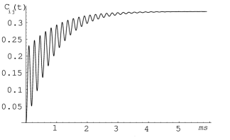
Figure 1: Conditional binary concurrence $C_{ij}(t)$ in correspondence to $N=3$, $\varepsilon=10^{5}Hz$, $k=10^{4}Hz$, $\Gamma=10^{3}Hz$ and $\omega=\tilde{\omega}_{0}=10^{14}Hz$

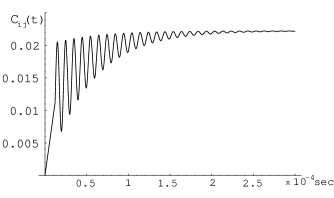
Figure 2: Conditional binary concurrence $C_{ij}(t)$ in correspondence to $N=10$, $\varepsilon=10^{5}Hz$, $k=10^{4}Hz$,$\Gamma=10^{3}Hz$ and $\omega=\tilde{\omega_{0}}=10^{14}Hz$

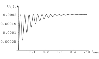
Figure 3: Conditional binary concurrence $C_{ij}(t)$ in correspondence to $N=10$, $\varepsilon=10^{5}Hz$, $k=10^{4}Hz$,$\Gamma=10^{3}Hz$ and $\omega=\tilde{\omega_{0}}=10^{14}Hz$

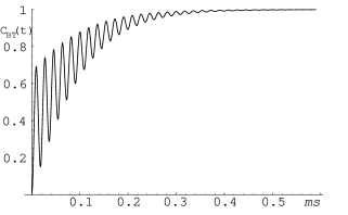
Figure 4: Total binary concurrence $C_{BT}(t)$ in correspondence to $N=3$, $\varepsilon=10^{5}Hz$, $k=10^{4}Hz$,$\Gamma=10^{3}Hz$ and $\omega=\tilde{\omega_{0}}=10^{14}Hz$

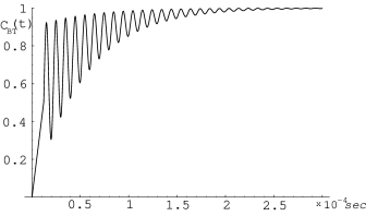
Figure 5: Total binary concurrence $C_{BT}(t)$ in correspondence to $N=10$, $\varepsilon=10^{5}Hz$, $k=10^{4}Hz$,$\Gamma=10^{3}Hz$ and $\omega=\tilde{\omega_{0}}=10^{14}Hz$

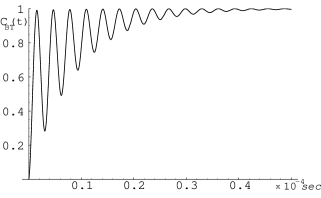
Figure 6: Total binary concurrence $C_{BT}(t)$ in correspondence to $N=100$, $\varepsilon=10^{5}Hz$, $k=10^{4}Hz$,$\Gamma=10^{3}Hz$ and $\omega=\tilde{\omega_{0}}=10^{14}Hz$

5 The asymptotic form of $\tilde{\rho}_{AC}$

It is of particular relevance that for

$$t\gg(k+N\Gamma)^{-1}\equiv\tau_{AC}$$ (46)

the correspondent asymptotic form assumed by $\tilde{\rho}_{AC}$ is time independent and such that the probability of finding energy in the effective JC subsystem exactly vanishes. Taking into account the easily demonstrable inequality $b<\tau_{AC}^{-1}$, it is immediate to convince oneself that for $t\gg\tau_{AC}$, the eq. (3) assumes the following diagonal asymptotic form

$$\tilde{\rho}_{AC}(t\gg\tau_{AC})=\left(\begin{array}[]{c c c c c c}\frac{1}{N}&0&0&...&0&0\\ 0&0&0&...&0&0\\ 0&0&\frac{1}{N}&...&0&0\\ \vdots&\vdots&\vdots&\vdots\vdots\vdots&\vdots&\vdots\\ 0&0&.&...&\frac{1}{N}&0\\ 0&0&.&...&0&0\end{array}\right)$$ (53)

Starting from eq. (53) and coming back to the old representation, it is possible to give at any time instant $t$ the exact solution $\rho_{AC}$ for the reduced density matrix of the system under scrutiny. Taking into account that the unitary operator $U$ is time independent, in view of eq. (53)

$$\rho_{AC}=U\tilde{\rho}_{AC}(t\gg\tau_{AC})U^{{\dagger}}$$ (54)

is time independent too. In fact we find that for $t\gg\tau_{AC}$, the reduced density matrix can be written in the compact form

$$\rho_{AC}=\frac{1}{N}|\beta_{1}\rangle\langle\beta_{1}|+\frac{N-1}{N^{2}}\sum_{h=2}^{N+1}|\psi_{T}^{(h)}\rangle\langle\psi_{T}^{(h)}|$$ (55)

$$\equiv\frac{1}{N}|\beta_{1}\rangle\langle\beta_{1}|+\frac{N-1}{N}\rho_{mix}$$

where

$$|\psi_{T}^{(h)}\rangle \equiv\frac{1}{\sqrt{N(N-1)}}\{(N-1)|\beta_{h}\rangle$$ (56)

$$-\sum_{j\neq h,j=2}^{N+1}|\beta_{j}\rangle\}\equiv|0\rangle|\varphi_{T}^{h}\rangle.$$

It is worth noting that each normalized state $|\varphi_{T}^{(h)}\rangle$ given by eq. (56), defines a particular subradiant Dicke state. It is indeed possible to prove that, whatever $N$ and $h$ are, the states $|\varphi_{T}^{(h)}\rangle$ are common eigenstates of $S_{z}$ and $S_{-}$ pertaining to eingevalues $-\frac{N-2}{2}$ and $0$ respectively. This property is a sufficient condition to claim that $|\psi_{T}^{(h)}\rangle$ is eigenstate of $\mathbf{S}^{2}$ too, having the form $|S,-S\rangle$ with $S=\frac{N-2}{2}$. This means that

$$\mathbf{S^{2}}\rho_{mix}\mathbf{S^{2}}=(S(S+1))^{2}\rho_{mix}$$ (57)

$$S_{z}\rho_{mix}S_{z}=S^{2}\rho_{mix}$$ (58)

and that each $|\psi_{T}^{(h)}\rangle$ defines an example of subradiand or trapped state Benivegna89 ; Dicke ; Dorris ; Tavis . Thus the result expressed by eq. (55) suggests that a statistical mixture of stationary subradiant Dicke states of the atomic sample, having well defined values of $\mathbf{S^{2}}$ and $S_{z}$, can be generated, at least in principle, putting outside the cavity single photon detectors allowing us to continuously monitor the decay of the system through the two possible channels (atomic and cavity dissipation) Carmichael . Eq. (55), indeed, clearly shows that, reading out the detectors state at $\bar{t}\gg\tau_{AC}$, if no photons has been emitted, then, as a consequence of this measurement outcome, our system is projected into the state $\frac{1}{N}\sum_{h=2}^{N+2}|\psi_{T}^{(h)}\rangle\langle\psi_{T}^{(h)}|$.

Stated another way, successful measurements, performed at large enough time instants $t$, generates an uncorrelated state of the two atomic and cavity field subsystems, leaving the matter sample in the statistical mixture of Dicke states $|\varphi_{T}^{(h)}\rangle$, satisfying eqs. (57) and (58). On the basis of the analysis reported in the previous section it is possible to state that such a statistical mixture is entangled.

Let’s finally observe that the probability $P$ that at $t=\bar{t}$ the excitation is still contained in the atomic system increases with the number $N$ of atoms, being $P=1-\frac{1}{N}$, as immediately deducible from eq. (55).

6 Conclusive Remarks

Summing up, in this paper we have exactly solved the dynamics of $N$ identical atoms resonantly interacting with a single mode cavity, taking into account from the very beginning the presence of both the resonator losses and the atomic spontaneous emission. We have moreover supposed that only one excitation is initially injected into the system of interest and that the atoms are located in such a way to experience the same cavity field.

From a mathematical point of view the novelty of our results is the presentation of an exact way to solve the master equation eq. (7) of the system, based on the unitary transformation accomplished by the operator U given by eq. (16). In the new representation associated to such a specific $U$, the differential equations governing the temporal behavior of the density matrix elements $\tilde{\rho}_{hj}$, become indeed much simpler to solve if compared with the ones ruling the temporal behavior of $\rho_{hj}$. This circumstance stems from the fact that in the new representation only one atom is at the same time coupled both to the cavity field and to the quantized electromagnetic modes of the thermal bath. The decoupling of the $N-1$ atoms is a direct consequence of the permutational symmetry properties acquired by the matter subsystem under the assumed point-like model condition.

From a physical point of view the new results reported in this paper have the merit of providing the key for transparently interpreting the origin of the asymptotic occurrence of collective subradiant Dicke behavior of the matter subsystem. The analysis and the discussion presented in section 4, highlighting some features of the entanglement formation process, legitimate the claim that the asymptotic condition toward which our physical system is guided by the loss mechanisms exhibits entanglement. It is of relevance to notice that the form of the stationary conditional state $\rho_{mix}$ appearing in eq. (55) is independent from both $\Gamma$ and $k$, while the exponential tendency toward the stationary condition is governed by the rate $k+N\Gamma$. This means that just the presence of only one loss channel is sufficient to address the same asymptotic radiation trapping condition, even if the transient duration is characterized by a different time decay constant. We wish in addition to emphasize that if the microscopic model neglects spontaneous atomic decay, cooperative effects occur even if the atomic sample is spatially dispersed Kozierowski ; Shore ; Kudryavstev ; Phoenix . On the contrary, the closeness of the $N$ atoms is a necessary requirement when the complete Hamiltonian model (2) is used (regardless of how bad the cavity is) in order that a robust entanglement may be conditionally reached in the matter subsystem. If indeed the distance among the $N$ atoms is larger than the radiation wavelength, collective behavior stemming from the interaction of each atom with a common bath, disappear with the consequence that the probability of finding in the system the initial energy goes toward zero with time. We thus may state that the key for trapping the energy in the atomic sample, inducing a stationary collective Dicke behavior, is the closeness among the atoms. We wish to conclude presenting some remarks concerning the experimental relevance of the problem discussed in this paper. We begin by observing that, in view of eq. (46), the value of $\tau_{AC}$ correspondent to $k=10^{4}Hz$ and $\Gamma=10^{3}Hz$ Pellizzari becomes much less than $10^{-2}$ whatever $N$ is. The experimental implementation of the specific conditions envisaged in our paper thus require the ability of locating for a time of the order of $10^{-2}sec$, $N$ atoms in an enough small region within an optical resonator. In particular the distance between two arbitrarily chosen atoms of our matter sample has to be much less than $500nm$. The more and more growing technological successes registered in the last few years in the confinement of individual atoms Balykin ; Chu ; 1atom ; 1atom2 or clouds of identical atoms Balykin ; Chu ; Ozeri with high spatial resolution, suggest that implementing our conditions in the near future is in the grasp of the experimentalists.To enforce our claim it is appropriate and relevant to quote the paper of Ozeri et al Ozeri wherein the authors experimentally demonstrate the possibility of confining in a blue-detuned optical trap a sample of $10^{5}$ Rubidium atoms in a region of $0.1\div 30nm$ for $0.3sec$ at a temperature of $24\mu K$.

References

- (1) A.Beige, Hugo Cable, P.L.Knight, in Proceeding of SPIE, 2003370, 5111 (2003)
- (2) A.Beige, Phys. Rev. A 67, 020301(R) (2003)
- (3) Guo Ping Guo et al, Phys. Rev. A 65, 042102 (2002)
- (4) Lu-Ming Duan et al, Phys. Rev. A 58, (1998)
- (5) T.Pellizzari, S.A.Gardiner, J.I.Cirac, P.Zoller, Phys. Rev. Lett. 75, 3788 (1995)
- (6) J.I.Cirac, P.Zoller, Phys. Rev. A 50, R2799 (1993)
- (7) S.Shneider, G.J.Milburn, Phys. Rev. A 65, 042107 (2002)
- (8) G.J.Yang, O.Zobay, P.Meystre, Phys. Rev. A 59, 4012 (1998)
- (9) E.Hagley, X.Maitre, G.Nogues, C.Wunderlich, M.Brune, J.M.Raimond, S.Haroche, Phys. Rev. Lett. 79, 1 (1997)
- (10) P.Foldi, M.G.Benedict, A.Czirjak, Phys. Rev. A 65, 021802 (2002)
- (11) M.B.Plenio, S.Huelga, A.Beige, P.L.Knight, Phys. Rev. A 59, 2468 (1999)
- (12) A.Beige, D.Braun, P.L.Knight, N.J.P. 2, 22.1-22.15 (2000)
- (13) Z.Ficek, R.Tanas, quant-ph0302124
- (14) L.Jakobczyk, J. Phys. A 35, 6383-6392 (2002)
- (15) Bo Yu, Zheng-Wei Zhou, Guang-Can Guo, J. Opt. B: Quantum Semiclass. Opt. 6, 86 (2004)
- (16) Jongcheol Hong, Hai-Woong Lee, Phys. Rev. Lett. 86, 237901 (2002)
- (17) S. Hill et al., Phys. Rev. Lett. 78, 5022-5025 (1997).
- (18) W. K. Wootters, Phys. Rev. Lett. 80, 2245-2248 (1998)
- (19) E.T.Jaynes and F.W.Cummings, Proc. IEEE 51, 89 (1963)
- (20) S.Haroche, in New Trends in Atomic Physics, Proceedings of the Les Houches Summer School of Theoretical Physics, Session XXXVIII, 1982, edited by G.Grynberg and R.Stora, (North-Holland, Amsterdam, 1982), p.193
- (21) C.Leonardi, F.Persico, G.Vetri, La rivista del Nuovo Cimento 9, (1986)
- (22) R. Friedberg, S. Hartmann, Phys. Rev. A 10, 1728 (1974)
- (23) A. Crubellier, J. Phys. B 20, 971 (1987)
- (24) H.Carmichael, An Open System Approach to Quantum Optics, Lectures Notes in Physics m18, (Springer-Verlag 1993)
- (25) Z.Ficek, R.Tanas, Phys. Rep. 372, 369-443 (2002)
- (26) F.Petruccione, H.P.Breuer, The Theory of open quantum system, (Oxford University Press, 2002)
- (27) W.H.Louisell, Quantum statistical properties of radiation, (John Wiley & Sons, 1973)
- (28) G.S.Agarval, Quantum Statistical Theories of Spontaneous Emission and their Relation to Other Approach, (Springer Tracts in Modern Physics, 1974)
- (29) G.Benivegna, A.Messina, Phys. Lett. A 126, 4 (1988)
- (30) V. Coffman, J. Kundu,W.K. Wootters, Phys. Rev. A 61, 052306 (2000)
- (31) K.A. Dennison, W.K. Wootters, Phys. Rev. A 65, 010301 (2001)
- (32) N. Linden, S. Popescu, W.K. Wootters, Phys. Rev.Lett. 89, 207901 (2002)
- (33) N. Linden, W.K. Wootters, Phys. Rev. Lett. 89, 277906 (2002)
- (34) M. Plesch, V. Buzek, Phys. Rev. A 67, 012322 (2003)
- (35) M. Plesch, V. Buzek, Phys. Rev. A 68, 012313 (2003)
- (36) M.H. Partovi, Phys. Rev. Lett. 92, 077904 (2004)
- (37) G.Benivegna, A.Messina, J. of Mod. Opt. 36, 1205 (1989)
- (38) R.H.Dicke, Phys. Rev. 93, 99 (1954)
- (39) F.W.Cummings, A.Dorris, Phys. Rev. A 28 , 2282 (1983)
- (40) F.W.Cummings, M.Tavis, Phys. Rev. 170, 379 (1968)
- (41) M.Kozierowsky, S.M.Chumakov, A.A.Mamedov, J. of Mod. Opt. 40, 453 (1993)
- (42) B.W.Shore, P.L.Knight, J. of Mod. Opt. 40, 7 (1993)
- (43) I.K.Kudryavstev, A.Lambrecht, H.Moya-Cessa, P.L.Knight, J. of Mod. Opt. 40, 8 (1993)
- (44) S.J.D.Phoenix, S.M.Barnett, J. of Mod. Opt. 40, 6 (1993)
- (45) V.I.Balykin, V.G.Minogin, V.S.Letokhov, Rep. Prog. Phys. 63, 1429 (2000)
- (46) S.Chu, Nature 416, 206 (2002)
- (47) N.Schlosser, G.Reymond, I.Protsenko, P.Grangier, Nature 411, 1024 (2001)
- (48) P.Maunz et al., Nature 428, 50 (2004)
- (49) R.Ozeri et al., Phys. Rev. A 59 , R1750 (1999)