Strong two-photon emission by a medium with periodically time-dependent refractive index

Abstract

A two-photon emission of a medium with periodically time-dependent refractive index is considered. The emission results from the zero-point fluctuations of the medium. Usually this emission is very weak. However, it can be strongly enhanced if the resonant condition $\omega_{0}$ = 2.94 $c/l_{0}$ is fulfilled (here $\omega_{0}$ and $l_{0}$ are the frequency and the amplitude of the oscillations of the optical length of the medium, respectively). Besides, a medium with resonant oscillations of the optical length performs the phase conjugated reflection with high efficiency. A similar resonant enhancement of the two-quantum emission of other bosons is also predicted.

The usual nonlinear optical processes leading to the generation of new waves, account for the stimulated emission Shen . Unlikely to that, the two-photon emission of a medium with the refractive index changing in time occurs due to the spontaneous emission arising from the zero-point fluctuations of the field Casimir ; Jablonovich ; quantopt . An interesting heuristic aspect of this emission is its close relation to some basic processes in quantum cosmology, e.g. to the creation of matter in the initial stage of the expanding universe quantopt . Besides, the change of $n$ linear in time results in the thermal-like radiation Jablonovich ”seen” by an observer when it moves with the constant acceleration Unruh ; this radiation is closely related to the Hawking radiation of black hole Birel .

As a rule, the two-photon emission under consideration is very weak. One can expect it to be observed only if the change of $n$ in time takes place in a large area and is very large and fast quantopt . The linear and strong time dependence of $n$ can be realized only in a small ”spot” in the medium for a very short time Jablonovich . Unlikely to that, the periodic and rather substantial oscillations of $n$ in time can be activated in a medium of a large size by applying a strong (quasi)monochromatic laser beam.

The size factor is of a primary importance here. Indeed, the oscillations of the refractive index in time lead also to oscillations of the optical length of the medium $l$. Taking $n(t)=n_{0}+n^{\prime}_{0}\cos{\omega_{0}t}$, we get for the time-dependent part of the optical length $l(t)=l_{0}\cos{\omega_{0}t}$, where $l_{0}=n^{\prime}_{0}L^{(0)}$, $\,L^{(0)}$ is the length of the coherently excited medium. Consequently, if $L^{(0)}$ is large then one can achieve large amplitude of the oscillations of the optical length $l_{0}$ even if $n^{\prime}_{0}$ is not too large. Therefore, the maximal velocity of the oscillations of the optical length $V=\omega_{0}l_{0}$ can also get large values which may be comparable, or even exceed the velocity of light in vacuum $c$. This has an important consequence: strong enhancement of the quantum emission if the maximal velocity $V$ of the oscillations of the optical length approaches $2.94c$. The reason for this resonant enhancement can be elucidated as follows. If $V\ll c$ then the intensity of the emission increases with $V$. However, if $V\gg c$, then the opposite dependence takes place, as the zero-point fluctuations cannot appreciably react on such a fast oscillations. Therefore, the crossover for the dependence of the emission on $V$ exists at $V_{r}\sim c$ and a resonant enhancement of it is observed at $V_{r}$. A possibility of the enhancement of the quantum emission in a dielectric medium with time-dependent parameters has been pointed out by a number of authors (see, e.g. Lobashov ; Klimov ; Johnston ; Saito ). But, in all previous studies this enhancement has been found to take place only in short resonator, which has discrete modes with well-separated frequencies; the enhancement is observed only for the mode, the multiple frequency of which is in resonance with $\omega_{0}$. For a given resonator there are series of modes and resonances; their frequencies are determined by the geometry of the resonator. The emission is non-stationary: the number of generated photons increases in time exponentially. However in our case the enhancement takes place only at $\omega_{0}=2.94c/n^{\prime}_{0}L_{0}$; the emission is stationary. Such a big difference of the properties of these phenomena results from the different mechanisms of the enhancement: in the case of a short resonator this is the parametric resonance for a time-dependent electromagnetic mode. The stimulated emission plays here an essential role: all generated photons remain in the resonator and essentially exert the process, resulting in the exponential increase of the number of photons in time. However in the case under consideration there is a continuum of modes which are mixed due to oscillations of $n$. The enhancement of the emission at $V=2.94c$ is due to the dynamical resonance of the zero-point fluctuations with the oscillations of the optical length. All generated photons immediately leave the region of generation and do not influence the process. Therefore, only a spontaneous emission contributes and the emission is stationary.

We are studying a medium exposed in a monochromatic standing laser wave. We describe the wave classically and account for the time-dependent part of the nonlinear polarization operator $\hat{P}^{(nl)}$. The equation for the field operator $\hat{A}$ then reads Shen $\ddot{\hat{A}}-(c/n_{0})^{2}\hat{\nabla}^{2}\hat{A}=-4\pi\ddot{\hat{P}}^{(nl)},$ where $\hat{P}^{(nl)}$ is the time-dependent part of the nonlinear polarization operator. We take $\hat{P}^{(nl)}(t)=\eta(t)\hat{A}/4\pi$, where $\eta(t)=\eta_{\,0}\,\cos{\omega_{0}t}$. Then we get

$$\ddot{\hat{A}}^{\prime}-(c/n(t))^{2}\hat{\nabla}^{2}\hat{A}^{\prime}=0,$$ (1)

where $\hat{A}^{\prime}=\hat{A}(1+\eta(t)),$ $\,n(t)=n_{0}\sqrt{1+\eta(t)}$. We suppose that $\eta_{0}\ll 1$; then $n(t)\approx n_{0}+n^{\prime}_{0}\cos{\omega_{0}t}$, where $n^{\prime}_{0}\approx\eta_{0}/2n_{0}$. Equation (1) is the wave equation with a harmonically time-dependent refractive index.

We are considering a dielectric situated in a very large resonator and suppose that the refractive index of the dielectric changes in time only in the time interval between $t=0$ and $t=t_{0}$. We want to find how this change influences upon the vacuum state of the quantum field at $t>t_{0}$. To this end, we use the Coleman theorem Coleman , which asserts that the time-dependent classical field leads to the change of the vacuum state in time. In our case this testify that the initial ($\hat{a}_{k},\,\hat{a}^{+}_{k}$) and final ($\hat{b}_{k},\,\hat{b}^{+}_{k}$) destruction and creation operators of a mode $k$ in the resonator are different Birel : they are related to each other by the Bogoljubov transformation

$$\hat{b}_{k}=\mu_{k}\,\hat{a}_{k}+\nu_{k}\,\hat{a}^{+}_{k},$$ (2)

where $|\mu_{k,q}|^{2}=1+|\nu_{k,q}|^{2}.$ This means that photons appear in the final state. The number of generated photons of the mode $k$ equals $N_{k}=\langle 0|\hat{b}^{+}_{k}\,(t)\,\hat{b}_{k}\,(t)|0\rangle=|\nu_{k}|^{2},$ where $|0\rangle$ is the initial zero-point state (in this state $\hat{a}_{k}|0\rangle=0$); the photons appear by pairs.

Usually, to find $N_{k}$, one calculates the parameters of the Bogoljubov transformation (2) (see, e.g. Birel ). However, there also exists another, a simpler way based on calculation of the pair correlation function

$${\cal D}_{k}(t;\tau)=\langle 0|\hat{A}_{k}(t+\tau)\hat{A}_{k}(t)|0\rangle$$ (3)

at a large time $t>t_{0}$, $\,\tau\ll t$ and with $t$ averaged over a period of oscillations euro ; here $\hat{A}_{k}(t)=(\hbar/2\omega_{k})^{1/2}\big{(}\hat{b}_{k}e^{-i\omega_{k}t}+\hat{b}^{+}_{k}e^{i\omega_{k}t}\big{)}\,$, $\omega_{k}$ is the frequency of the mode $k$. Indeed, inserting Eq. (2) into Eq. (3) we find

$${\cal D}_{k}(t;\tau)=(\hbar/2\omega_{k})\big{(}|\mu_{k}|^{2}e^{-i\omega_{k}\tau}+|\nu_{k}|^{2}e^{i\omega_{k}\tau}\big{)},$$ (4)

(the terms $\propto e^{\pm 2i\omega_{k}t}$ drop out). Consequently, to find the number of the generated photons $N_{k}$, one may calculate the negative frequency (with respect to $\tau$) term of the large-time $t$ asymptotic of the pair correlation function ${\cal D}_{k}(t;\tau)$. Below we will use this method to calculate the quantum emission under consideration.

We suppose that $n^{\prime}_{0}$ very slowly changes in space. Then, according to the theory of the wave-optics Solimeno the plane waves $\hat{A}_{q}(x,t)\propto e^{iqx}$ are the solutions of this equation outside the medium (then the operators $\hat{A}^{\prime}$ and $\hat{A}$ coincide); at that the allowed values of the wave number $q$ satisfy the condition $qL(t)=2\pi k$, where $k=0,1,2\dots,$ $L(t)=L_{0}+l(t)$ is the optical length (eikonal) of the resonator + dielectric at time $t$. Therefore the field operator outside the medium has the form

$$\hat{A}(x,t)=\sum_{k}\sin{(\pi kx/L(t))}\hat{A}_{k}(t)..$$

This operator satisfies the wave equation in vacuum $\ddot{\hat{A}}-c^{2}\nabla^{2}\hat{A}=0$ which gives in the $L/l_{0}\rightarrow\infty$ limit

$$\sum_{k}\bigg{[}\ddot{\hat{A}}_{k}+\omega^{2}_{k}\hat{A}_{k}-\frac{k\pi x}{L^{2}}\big{(}2\dot{L}\dot{\hat{A}}_{k,{\vec{q}}}+\ddot{L}\hat{A}_{k}\big{)}\cot{\bigg{(}\frac{\pi kx}{L}\bigg{)}}\bigg{]}=0,$$ (5)

where $\omega_{k}=\pi ck/L_{0}$ (the terms $\propto L^{-m}$ with $m>2$ are neglected). Taking into account the identity

$$\pi x/L=-2\sum_{j=1}^{\infty}(-1)^{j}j^{-1}\sin{(\pi jx/L)},\quad-L\leq x\leq L,$$

one gets for $\hat{{\cal A}}_{k}=(-1)^{k}\hat{A}_{k}$  the equation $\ddot{\hat{\cal A}}_{k}+\omega^{2}_{k}\hat{\cal A}_{k}\simeq\omega_{k}\hat{B}_{k},$ where

$$\hat{B}_{k}=(2/\pi c)\sum_{j\neq k}j(2\dot{L}\,\dot{\hat{{\cal A}}}_{j}+\ddot{L}\,\hat{{\cal A}}_{j})/(j^{2}-k^{2}).$$

We consider the case when the oscillations of $n$ last for a long time $t_{0}$. Using the Green function of the harmonic oscillator $\omega_{k}^{-1}\Theta{(t)}\sin{\omega_{k}t}$, where $\Theta{(t)}$ is the Heaviside step-function, we get for $t\geq t_{0}$

$$\hat{{\cal A}}_{k}(t)\simeq\hat{{\cal A}}^{(0)}_{k}(t)+\int_{0}^{t_{0}}\!\!\!dt_{1}\sin{(\omega_{k}(t-t_{1}))}\!\hat{B}_{k}(t_{1}),$$ (6)

where $\hat{{\cal A}}^{(0)}_{k}(t)=(-1)^{k}(\hbar/2\omega_{k})(\hat{a}_{k}e^{-i\omega_{k}t}+\hat{a}^{+}_{k}e^{i\omega_{k}t})$. From Eq. (6) it follows that in the $t\rightarrow\infty$ limit the operator $\hat{\cal A}_{k}(t)$ consists of two items: the positive frequency item $\propto e^{-i\omega_{k}\,t}$ and the negative frequency item $\propto e^{i\omega_{k,\vec{q}}\,t}$. Besides, in the large $t_{0}$ limit the main contribution to the integral (6) comes from large $t_{1}$. In this case the time-dependence of the factors $\hat{{\cal A}}_{j}$ entering the equation for $\hat{B_{k}}$, is given by the exponents $e^{\pm i\omega_{k}\,t_{1}}$. We also take into account that in the large $t_{0}$ limit only the terms with $\omega_{k}+\omega_{j}=\omega_{0}$ make a remarkable contribution to the integral in Eq. (6). Therefore the only essential contribution to this integral comes from the terms with $L(t_{1})\hat{{\cal A}}_{j,{\vec{q}}}(t_{1})\propto\exp{(\pm i(\omega_{0}-\omega_{j})t_{1})}$ (the terms $\propto\exp{(\pm i(\omega_{j}+\omega_{0})t_{1})}$ are averaged out at the large $t_{0}$ limit). In this case $\,2\dot{L}(t_{1})\,\dot{\hat{{\cal A}}}_{j}\,(t_{1})+\ddot{L}(t_{1})\,\hat{{\cal A}}_{j}\,(t_{1})\propto j^{2}-k^{2}$. As a result the factor $j^{2}-k^{2}$ in the equation for $\hat{B}_{k}$ cancels and the $k$-dependence disappears:

$$\hat{B}\,(t)=2V\cos{(\omega_{0}t)}\hat{Q};\quad\hat{Q}=\kappa_{0}^{-1}L_{0}^{-1}\sum_{j=1}j\hat{{\cal A}}_{j}.\,$$ (7)

Here $\hat{Q}$ is the operator of the wave packet of the size $\sim k_{0}^{-1}$, where $\,\kappa_{0}=\omega_{0}L_{0}/\pi c$.

Eq. (7) for $\hat{B}$ is the key relation of this study: it accounts for the effect of the oscillations of the optical length in the case of an infinitely large resonator. This relation essentially differs from the analogous relation, describing this effect in the case of a short resonator, which has been studied earlier Lobashov ; Klimov ; Johnston ; Saito : in the latter case the contribution of only one (or few) so-called ”resonant” mode(s) $j$ into the operator $\hat{B}_{k}$ is taken into account. However in the case under consideration there is a continuum of modes which all are essentially mixed by the oscillations of the optical length. Therefore, they all contribute to $\hat{B}$. This circumstance becomes especially clear if one considers the effective Hamiltonian

$$\hat{H}=\frac{1}{2}\sum_{k}(\dot{\hat{A}}^{2}_{k}+\omega_{k}^{2}\hat{A}^{2}_{k})-V\omega_{0}L_{0}\cos{(\omega_{0}t)}\,\hat{Q}^{2}$$ (8)

which corresponds to the equation of motion (6) and the given $\hat{B}$. Here the last term describes the effective interaction between the modes arising from the oscillations of the optical length. One can see that this interaction is factorized; all modes contribute to the factors of this interaction. We note that Hamiltonian (8) is analogous to the one describing the two-phonon decay of a local mode in a crystal. This allows one to apply the method proposed in Hizhrev ; EPJ for a nonperturbative description of this decay.

To find the number of generated photons, one may diagonalize the Hamiltonian (8) (it is done in Hizhrev ). However one can find $N_{k}$ directly from equations (6), (7) and (4):

$$N_{k}\simeq\frac{V^{2}\omega_{k}}{2\hbar}\int\!\!\!\!\!\int_{0}^{t_{0}}\!\!\!\!\!dt_{1}dt^{\prime}_{1}e^{i(\omega_{0}-\omega_{k})(t_{1}-t^{\prime}_{1})}D(t_{1},t^{\prime}_{1}).$$ (9)

Here $D(t,t^{\prime})=\langle 0|\hat{Q}(t_{1})\hat{Q}(t^{\prime}_{1})|0\rangle$; in the $t_{0}\rightarrow\infty$ limit this correlation function depends on the time difference. The emission rate $\dot{N}_{k}=dN_{k}/dt_{0}$ now equals

$$\dot{N}_{k}=(V^{2}/2\hbar)\,\omega_{k}D(\omega_{0}-\omega_{k}),$$

where $D(\omega)$ is the Fourier transform of the correlation function $D(t-t^{\prime})$; here $\omega$ and $\omega_{0}-\omega$ are the frequencies of two emitted photons. Thus, to find the quantum emission under consideration, one needs to calculate the correlation function $D(\omega)$. If $V\ll c$ then one can replace in Eq. (7) for $\hat{Q}$ the field operator $\hat{{\cal A}}_{j}$ by $\hat{{\cal A}}_{j}^{(0)}$. In this approximation $D(\omega)\approx\hbar\omega/2\pi^{2}c^{2}\omega_{0}^{2}$ and

$$\dot{N}(\omega)\approx(v/2\pi\omega_{0})^{2}\,\omega(\omega_{0}-\omega)$$

($v=V/c$). This equation coincides with that given by the standard time-dependent perturbation theory. We can see that the emission under consideration is very different from the one in small resonator: it is stationary, its spectrum is broad, while in the case of a small resonator, in the resonance conditions, it is non-stationary and quasi-monochromatic.

To find the emission for an arbitrary $V$, we follow the calculations given in EPJ (see part 2.2.1, the k=2 case). We use the equation of motion for the operator $\hat{Q}$ :

$$\hat{Q}(t)=\hat{Q}^{(0)}(t)+2v\omega_{0}\!\!\int_{0}^{t}\!\!\!\!dt_{1}G(t-t_{1})\cos{(\omega_{0}t_{1})}\hat{Q}(t_{1})$$ (10)

($t\leq t_{0}$), which directly follows from Eqs. (6) - (7). Here $\hat{Q}^{(0)}$ is given by Eq. (7) for $\hat{Q}$ with $\hat{{\cal A}}_{j}^{(0)}$ instead of $\hat{{\cal A}}_{j}$,

$$G(t)=({\rm\Theta}(t)/\pi\kappa_{0}^{2})\sum_{k=1}^{\kappa_{0}}k\sin{\omega_{k}t}$$

is the Green function. Using Eq. (10) once again (this time for $\hat{Q}(t_{1})$) and inserting it into $D(t,t^{\prime})$ we find

$$D(t,t^{\prime})\simeq d(t,t^{\prime})+2v\omega_{0}\int_{0}^{t}\!\!\!\!dt_{1}G(t-t_{1})\cos{(\omega_{0}t_{1})}D_{1}^{*}(t_{1},t^{\prime})$$

$$+v^{2}\omega_{0}^{2}\int_{0}^{t}\!\!\!\!dt_{1}\!\!\int_{0}^{t_{1}}\!\!\!\!\!\!\!dt_{2}G(t-t_{1})G(t_{1}-t_{2})e^{-i\omega_{0}(t_{1}-t_{2})}D(t_{2},t^{\prime}),$$

where $d(t,t^{\prime})=\langle 0|\hat{Q}^{(0)}(t)\hat{Q}(t^{\prime})|0\rangle$, and an analogous equation for $d^{*}(t^{\prime},t)$. We take into account only $e^{i\omega_{0}(t_{1}-t_{2})}$ term of the factor $4\cos{(\omega_{0}t_{1})}\cos{(\omega_{0}t_{2})}$; other terms oscillate fast and drop out. Above the term $\propto v$ may be omitted while it also oscillates fast. Taking into account that in the large time limit the correlation functions $D(t,t^{\prime})$ and $d(t,t^{\prime})$ depend on the time difference and using the relations

$$\int_{0}^{\infty}\!\!\!\!\!\!dt\!\!\int_{0}^{t}\!\!\!\!dt_{1}\!\!\int_{0}^{t_{1}}\!\!\!\!\!\!\!dt_{2}e^{i\omega t}=\int_{0}^{\infty}\!\!\!\!\!\!\!dt_{2}e^{i\omega t_{2}}\!\!\int_{0}^{\infty}\!\!\!\!\!\!d\tau_{1}e^{i\omega\tau_{1}}\!\!\int_{0}^{\infty}\!\!\!\!\!\!\!d\tau e^{i\omega\tau}$$

$$\int_{0}^{\infty}\!\!\!\!\!\!dte^{i\omega t}F(t-t^{\prime})\simeq e^{i\omega t^{\prime}}\!\!\int_{-\infty}^{\infty}\!\!\!\!\!\!d\tau e^{i\omega\tau}F(\tau)=e^{i\omega t^{\prime}}F(\omega)$$

($t^{\prime}\rightarrow\infty,\,\tau=t-t_{1},\,\tau_{1}=t_{1}-t_{2}$), one gets the following equation for $D(\omega)$ Hizhrev ; EPJ ; euro (the factor $e^{i\omega t^{\prime}}$ cancels):

$$D(\omega)\simeq d(\omega)+v^{2}G(\omega)G(\omega-1)D(\omega),$$

where

$$G(\omega)=\frac{1}{\pi}\bigg{[}1+\frac{\omega}{2}\ln{\frac{|1-\omega|}{|1+\omega|}}\bigg{]}+\frac{i\omega}{2}\,\Theta{(1-|\omega|)},$$

and an analogous equation for $d^{*}(\omega)$ (we take $\omega_{0}=1$ for the frequency units). As a result, the number of the emitted photons with the frequency $\omega$ per unit time and frequency equals:

$$\dot{N}(\omega)=\frac{(v/2\pi)^{2}\omega(1-\omega)}{|1-v^{2}G^{*}(\omega)G(1-\omega)|^{2}}.$$ (11)

This expression describes the emission under consideration for any value of $v$. If $v\ll 1$, then the intensity of the emission increases quadratically with $v$. However, if $v\gg 1$, then the dependence on $v$ is the opposite: $\dot{N}\propto v^{-2}$. If $v$ approaches the value

$$v_{r}=4\pi/\sqrt{\pi^{2}+(4-\ln{3})^{2}}\approx 2.94,$$

then the resolvent at $\omega=$ 1/2 diverges and the emission is resonantly enhanced (see Figs. 1 and 2). The given value of $v_{r}$ is close to $\pi$, i.e. the value of $v$ which corresponds to the resonance between the oscillations of the optical length and the generated wave, when the distance between the turning points of $l$ coincides with the half-wave of the generated photons.

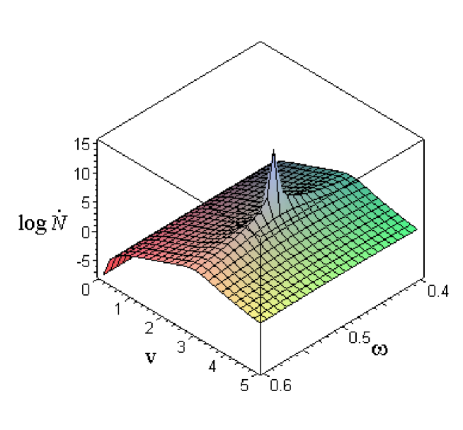
Figure 1: The logarithm of the rate of the emission of photons $\dot{N}$ by a medium with time-dependent refractive index $n=n_{0}+n^{\prime}_{0}\cos{\omega_{0}t}$, as a function of the frequency of emission $\omega$ and maximal velocity $v$ of the optical length (the units $\omega_{0}=1$ and $c=1$ are used).

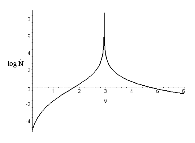
Figure 2: The logarithm of the integrated rate of the emission of photons $\dot{\rm N}=\int\!\!\dot{N}(\omega)d\omega$ by a medium with time-dependent refracting index, as a function of the maximal velocity $v$ of the optical length (the same units as in Fig. 1 are used).

To estimate the intensity of a laser beam which can give $v=n^{\prime}_{0}\omega_{0}L^{(0)}/c\sim 1$ and which can cause the resonant enhancement of the two-photon emission, we take $n^{\prime}_{0}\sim n^{(2)}I$, where $I$ is the intensity of the laser light, $n^{(2)}\sim 10^{-15}cm^{2}/W$, - a typical non-resonant value of $n^{(2)}$ in crystals Shen . We also take $\omega_{0}L^{(0)}/c\sim 10^{5}$and $n^{(2)}\sim 10^{-15}cm^{2}/W$. We get $I\sim 10^{10}W/cm^{2}$. Such intensity of the laser light is experimentally achievable.

In our consideration we describe the emission in the direction $x$, which was chosen arbitrarily. This means that photons are emitted in all directions. The positive and the negative direction along the $x$ axis are not distinguished in our case. Therefore the pairs of photons with the wave vectors $\pm{\vec{q}}$ and $\pm\alpha{\vec{q}}$ along the $x$ axis are equally generated by the medium (here $\alpha=\omega_{0}/\omega-1$).

Only a spontaneous emission was considered above. If $N_{\vec{q}}$ photons with the wave-vector ${\vec{q}}$ and the frequency $\omega=cq<\omega_{0}$ are fall into a medium with $n$ oscillating in time, then also stimulated processes give a contribution to the emission. As a result, an additional factor $1+N_{\vec{q}}$ appears in the equation for the intensity of the emission of photons with the wave-vectors ${\vec{q}}$ and ${\vec{q}}=-\alpha{\vec{q}}$, where $\alpha=\omega_{0}/\omega-1$. It is essential to underline that the presence of photons with the wave-vector ${\vec{q}}$ leads to an enhancement of the emission of photons not only with the same wave vector but also of photons with the wave-vector $-\alpha{\vec{q}}$. E.g. the photons with the wave number $q=\omega_{0}/2c$ do stimulate the emission of photons with the wave vector $=-{\vec{q}}$. This is a well-known fact Pepper : a medium with a refractive index oscillating in time performs the phase-conjugated reflection of photons with half a frequency. In our case, in the resonance condition it takes place with a high efficiency.

A medium with oscillating refractive index is not the only physical system where the optical length oscillates in time; a resonator with vibrating mirror(s) gives another example. In the latter case the maximal velocity of the oscillations of the mirror(s) is limited by the velocity of light. However a reflecting border in a dielectric medium can be put to oscillate with $V>c$, e.g. by means of a strong laser beam which periodically changes its direction so that the position of the area, being illuminated by the beam, moves forth and back with $V>c$. In this case one can get strong enhancement of the two-photon emission if $V$ approaches $2.9c$. Note also that in a small resonator (cavity) with vibrating walls one can also get strong enhancement of the generation of photons of a mode if it is in parametric resonance with the oscillations (see, e.g. Casimir ; Law ; More ; Janovich ; Mundarain ; Dodonov ; Jenson ; Visser ; Jacobs ; Rzazewski ; Schaller ).

Finally, we note that the emission under consideration can be generated by any strong coherent long-wave excitation, which periodically modulates $n$. A similar emission of other bosons as well as the resonant enhancement of this emission is also possible in a periodically time-dependent medium, analogously to the above-described resonant enhancement of the two-photon emission. To prove the aforementioned we consider the quantum field, which satisfies the time-dependent Klein-Gordon equation

$$[\partial^{2}/\partial t^{2}-c^{2}\hat{\nabla}^{2}+m^{2}]\hat{A}=-\partial^{2}\eta(t)\hat{A}/\partial t^{2}.$$

In this case the above presented consideration of the two-quantum emission holds also if one replaces the frequency of a photon $\omega=cq$ by the frequency of the particle $\sqrt{c^{2}q^{2}+m^{2}}$. The number of the emitted quanta (particles and antiparticles) in the time unit is also described by the Eq. (11) if $G(\omega)$ is replaced by the difference $G(\omega)-G_{1}(\omega)$ where $G_{1}(\omega)$ can be obtained from $G(\omega)$ by replacing $1-\omega$ by $2m-\omega$; the two-particle emission under consideration exists only if the rest mass of the particle-antiparticle pair $2m$ (in the $\omega_{0}=\hbar=c=1$ units) does not exceed $1$. This result may be of interest to the physics of condensed matter, e.g. to the generation of phonon pairs in a semiconductor by a strong microwave or to a two-phonon decay of the strong phonon wave generated in CARS experiments. It may also offer interest for the astrophysics as a possible mechanism of a powerful emission of particles.

To sum up, a solution of the problem of the two-quantum emission of a periodically time-dependent medium has been given. It has been found that, if the maximal value of the velocity of the oscillating optical length approaches the critical value 2.94$c$, then a strong enhancement of the two-photon emission takes place. It has also been found that a medium with the resonant oscillations of the refractive index may carry out the phase-conjugated reflection with high efficiency. A similar resonant enhancement of other types of two-quantum emission has also been predicted.

Acknowledgement. The research was supported by the ETF Grant No 5023 and by the US NRC Twinning Program.

References

• (1) Y.R.ย Shen, The principles of nonlinear optics, University of California, Berkeley, John Wiley and Sons, Inc., 1984.
• (2) M.ย Bordag (editor), The Casimir Effect 50 Years Latter, Proceedings of the Fourth Workshop on Quantum Field Theory under the Influence of External conditions (World Scientific, 1999).
• (3) E.ย Jablonovitch, Phys. Rev. Lett. 62, 1742 (1989).
• (4) V.ย Hizhnyakov, Quantum Opt. 4, 277 (1992).
• (5) W.G.ย Unruh, Phys. Rev. D, 14, 870 (1967).
• (6) N.D.ย Birel and P.C.W.ย Davies, Quantum Fields in Curved Space, Cambridge University Press, Cambridge, 1982.
• (7) A.A.ย Lobashov and V.V.ย Mostepanenko, Teor. Mat. Fiz. 86, 438 (1991); 88 913 (991) (Theor. and Math. Phys. 86, 303 (1991); 88 340 (991)).
• (8) V.V.ย Dodonov, A.B.ย Klimov and D.E.ย Nikonov, Phys. Rev., A 47, 4422 (1993).
• (9) H.ย Johnston and S.ย Sarker, Phys. Rev. A 51, 4109 (1995).
• (10) H.ย Saito, and H. Hyuga, J. Phys. Soc. Japan, 65, 1139, 3513 (1996).
• (11) S.ย Coleman, J. Math. Phys. 7 787 (1967).
• (12) V.ย Hizhnyakov, Europhys. Lett., 45, 508 (1999).
• (13) S.ย Solimeno, B.ย Crosignani, P.ย DiPorto, Guiding, Refraction, and Confinement of Optical Radiation, Academic Press, INC., 1998.
• (14) V.ย Hizhnyakov, Phys.Rev. B 53, 13981 (1996).
• (15) V.ย Hizhnyakov, H.ย Kaasik, I.ย Tehver, Eur. Phys. J. B 28, 271 (2002).
• (16) D.M.ย Pepper, Nonlinear Optical Phase Conjugation. - Opt. Engineering, 1982, 21, 156.
• (17) G.T.ย More, J. Math. Phys 11, 2679 (1970).
• (18) C.K.ย Law, Phys. Rev. A 49, 433 (1994); A 51, 2537 (1995).
• (19) M.ย Janovich, Phys. Rev. A 57, 4784 (1998).
• (20) D.F.ย Mundarain, P.A.ย Maia Neto, Phys. Rev.A 57, 1379 (1998).
• (21) V.V.ย Dodonov, Phys. Lett. A 244, 517 (1998); Adv. Chem. Phys. 119, 309-394, Part 1, Sp. Iss. 2 (2001).
• (22) B.ย Jenson, I.ย Brevik, Phys. Rev. E 61, 6639 (1999).
• (23) M.ย Visser, S.ย Liberati, F.ย Belgiorno, D.W.ย Sciarna, Phys. Rev. Lett. 83, 678 (1999).
• (24) K.ย Jacobs, I.ย Tittonen, H.M.ย Wiseman, Phys. Rew. A 60, 538 (1999).
• (25) M.ย Cirone, K.ย Rzazewski, Phys. Rev. A 60, 886 (1999).
• (26) G.ย Schaller, R.ย Sch tzhold, G.ย Plunien, G.ย Soff, Phys. Let. A 297, 81 (2002).