Testing the bounds on quantum probabilities

Abstract

Bounds on quantum probabilities and expectation values are derived for experimental setups associated with Bell-type inequalities. In analogy to the classical bounds, the quantum limits are experimentally testable and therefore serve as criteria for the validity of quantum mechanics.

I Introduction

Suppose someone claims that the chances of rain in Vienna and Budapest are 0.1 in each one of the cities alone, and the joint probability of rainfall in both cities is 0.99. Would such a proposition appear reasonable? Certainly not, for even intuitively it does not make much sense to claim that it rains almost never in one of the cities, yet almost always in both of them. The worrying question remains: which numbers could be considered reasonable and consistent? Surely, the joint probability should not exceed any single probability. This certainly appears to be a necessary condition, but is it a sufficient one? In the middle of the 19th century George Boole, in response to such queries, formulated a theory of “conditions of possible experience” Boole (1958, 1862) which dealt with this problem. Boole’s requirements on the (joint) probabilities of logically connected events are expressed by certain equations or inequalities relating those (joint) probabilities.

Since Bell’s investigations Bell (1987); Clauser and Shimony (1978); Peres (1993) into bounds on classical probabilities, similar inequalities for a particular physical setup have been discussed in great number and detail. In what follows, the classical bounds are referred to as “Bell-type inequalities.” Whereas these bounds are interesting if one wants to inspect the violations of classical probabilities by quantum probabilities, the validity of quantum probabilities and their experimental verification is a completely different issue. Here we shall present detailed numerical studies on the bounds of quantum probabilities which, in analogy to the classical bounds, are experimentally testable.

I.1 Correlation Polytopes

In order to establish bounds on quantum probabilities, let us recall that Pitowsky has given a geometrical interpretation of the bounds of classical probabilities in terms of correlation polytopes Pitowsky (1986, 1989a, 1989b, 1991, 1994) [see also Froissart Froissart (1981) and Tsirelson (also spelled Cirel’son) Cirel’son (1980); Cirel’son (1993) (=Tsirelson)].

Consider an arbitrary number of classical events $a_{1},a_{2},\ldots,a_{n}$. Take some (or all of) their probabilities and some (or all of) the joint probabilities $p_{1},p_{2},\ldots,p_{n},p_{12},\ldots$ and identify them with the components of a vector $p=(p_{1},p_{2},\ldots,p_{n},p_{12},\ldots)$ formed in Euclidean space. Since the probabilities $p_{i}$, $i=1,\ldots,n$ are assumed to be independent, every single one of their extreme cases $0,1$ is feasible. The combined values of $p_{1},p_{2},\ldots,p_{n}$ of the extreme cases $p_{i}=0,1$, together with the joined probabilities $p_{ij}=p_{i}p_{j}$ can also be interpreted as rows of a truth table; with $0,1$ corresponding to “false” and “true,” respectively. Moreover, any such entry corresponds to a two-valued measure (also called valuation, 0-1-measure or dispersionless measure).

In geometrical terms, any classical probability distribution is representable by some convex sum over all two-valued measures characterized by the row entries of the truth tables. That is, it corresponds to some point on the face of the classical correlation polytope $C={\rm conv}(K)$ which is defined by the set of all points whose convex sum extends over all vectors associated with row entries in the truth table $K$. More precisely, consider the convex hull ${\rm conv}(K)=\left\{\sum_{i=1}^{2^{n}}\lambda_{i}{\bf x}_{i}\;\left|\;\lambda_{i}\geq 0,\;\sum_{i=1}^{2^{n}}\lambda_{i}=1\right.\right\}$ of the set

$$K=\{{\bf x}_{1},{\bf x}_{2},\ldots,{\bf x}_{2^{n}}\}=\left\{\left.\large(t_{1},t_{2},\ldots,t_{n},t_{x}t_{y},\ldots\large)\;\right|\;t_{i}\in\{0,1\},\;i=1,\ldots,n\right\}.$$

Here, the terms $t_{x}t_{y},\ldots$ stand for arbitrary products associated with the joint propositions which are considered. Exactly what terms are considered depends on the particular physical configuration.

By the Minkoswki-Weyl representation theorem (Ziegler, 1994, p.29), every convex polytope has a dual (equivalent) description: (i) either as the convex hull of its extreme points; i.e., vertices; (ii) or as the intersection of a finite number of half-spaces, each one given by a linear inequality. The linear inequalities, which are obtained from the set $K$ of vertices by solving the so called hull problem coincide with Boole’s “conditions of possible experience.”

For particular physical setups, the inequalities can be identified with Bell-type inequalities which have to be satisfied by all classical probability distributions. These conditions are demarcation criteria; i.e., they are complete and maximal in the sense that no other system of inequality exist which characterizes the correlation polytopes completely and exhaustively (That is, the bounds on probabilities cannot be enlarged and improved). Generalizations to the joint distributions of more than two particles are straightforward. Correlation polytopes have provided a systematic, constructive way of finding the entire set of Bell-type inequalities associated with any particular physical configuration Pitowsky and Svozil (2001); Filipp and Svozil (2003), although from a computational complexity point of view Garey and Johnson (1979), the problem remains intractable Pitowsky (1991).

I.2 Quantum Probabilities

Just as the Bell-type inequalities represent bounds on the classical probabilities or expectation values, there exist bounds on quantum probabilities. In what follows we shall concentrate on these quantum plausibility criteria, in particular on the bounds characterizing the demarcation line for quantum probabilities.

Although being less restrictive than the classical probabilities, quantum probabilities do not violate the Bell-type inequalities maximally Popescu and Rohrlich (1994); Mermin (1995); Krenn and Svozil (1998). Tsirelson Cirel’son (1980); Cirel’son (1993) (=Tsirelson); Khalfin and Tsirelson (1992) as well as Pitowsky Pitowsky (2002) have investigated the analytic aspect of bounds on quantum correlations. Analytic bounds can also be obtained via the minmax principle (Halmos, 1974, §90), stating that the the bound (or norm) of a self-adjoint operator is equal to the maximum of the absolute values of its eigenvalues. The eigenvectors correspond to pure states associated with these eigenvalues. Thus, the minmax principle is for the quantum correlation functions what the Minkoswki-Weyl representation theorem is for the classical correlations. Werner and Wolf Werner and Wolf (2001), as well as Cabello Cabello (2003), have considered maximal violations of correlation inequalities, and have also enumerated quantum states associated with extreme points of the convex set of quantum correlation functions.

The maximal violation of the Clauser-Horne-Shimony-Holt (CHSH) inequality involving expectation values of binary observables is related to Grothendieck’s constant Fishburn and Reeds (1994). But the demarcation criteria for quantum probabilities are still far less understood than their classical counterparts. In a broader context, Cabello has described a violation of the CHSH inequality beyond the quantum mechanical (Tsirelson’s) bound by applying selection schemes to particles in a GHZ-state Cabello (2002a, b), yet here we only deal with the usual quantum probabilities of events which are not subject to selection procedures.

To be more precise, consider the set of all single particle probabilities $q_{i}={\rm tr}[W(E_{i}\otimes{\mathbb{I}})]$ and ${\rm tr}[W({\mathbb{I}}\otimes F_{i})]$, as well as the two particle joint probabilities $q_{ij}={\rm tr}[W(E_{i}\otimes F_{j})]$, where some $E_{i}$, $F_{j}$ are projection operators on a Hilbert space $H$, and $W$ is some state on $H\otimes H$. Again, generalizations to the joint distributions of more than two particles are straightforward. An analogue to the classical correlation polytope $C$ is the set of all quantum probabilities

$$\begin{array}[]{l}Q=\left\{\left.\large(q_{1},q_{2},\ldots,q_{n},q_{xy},\ldots\large)\;\right|\;q_{i}={\rm tr}[W(E_{i}\otimes{\mathbb{I}})]\;{\rm or}\;\;{\rm tr}[W({\mathbb{I}}\otimes F_{i})],\;q_{ij}={\rm tr}[W(E_{i}\otimes F_{j})]\right\},\end{array}$$

with $E_{i}E_{i}=E_{i},\;F_{j}F_{j}=F_{j}$, $W^{\dagger}=W,\;{\rm tr}(W)=1$, and $\langle u|W|u\rangle\geq 0$, $i,j=1,\ldots,n$ for all $|u\rangle\in H\otimes H$. The vertices of classical correlation polytopes $C$ coincide with points of $Q$, if $E_{i},F_{j}\in\{{\rm diag}(0,\ldots,0),{\mathbb{I}}={\rm diag}(1,\ldots,1)\}$, where ${\rm diag}(a,b,\ldots)$ stands for the diagonal matrix with diagonal entries $a,b,\ldots$; in these cases, $W$ may be arbitrary. A proof of the convexity of $Q$ can be found in Pitowsky (2002). Notice, however, that geometrical objects derived from expectation values need not be, and in fact are not convex, as an example below shows.

One could obtain an intuitive picture of $Q$ by imagining it as an object (in high dimensions) created from “soap surfaces” which is suspended on the edges of $C$, and which is blown up with air: the original polytope faces which are hyperplanes get “bulged” or “curved out” such that, instead of a single plane per face, a continuity of tangent hyperplanes are necessary to characterize it Khalfin and Tsirelson (1992).

II Numerical studies

In what follows, we shall first consider the parameterization of projections and states. The numerically calculated expectation values obey the Tsirelson bound, exceeding the values for the classical Clauser-Horne-Shimony-Holt (CHSH) inequality. Then, we shall deal with the Clauser-Horne (CH) inequality and a higher dimensional example taken from Pitowsky and Svozil (2001) in more detail, followed by an attempt to depict the convex body $Q$ itself.

II.1 Parameterization

Consider a two spin-1/2 particle configuration, in which the two particles move in opposite directions along the $y$-axis, and the spin components are measured in the $x$–$z$ plane, as depicted in Figure 1.

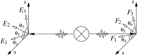
Figure 1: Measurements of spin components corresponding to the projections ${E}_{i}$ and ${F}_{j}$.

In such a case, the single-particle spin observables along $\theta$ correspond to the projections $E_{i}$ and $F_{j}$; i.e., $E_{i},F_{j}=E(\theta_{i}),F(\theta_{j})$ with

$$E(\theta)=F(\theta)=\frac{1}{2}({\mathbb{I}}+{\bf n}(\theta)\cdot{\bf\sigma})=\frac{1}{2}\left(\begin{array}[]{cc}1+\cos\theta&\sin\theta\\ \sin\theta&1-\cos\theta\end{array}\right),$$ (1)

where ${\bf\sigma}$ is the vector composed from the Pauli spin matrices.

Any state represented by the operator $W$ must be (i) self-adjoint $W^{\dagger}=W$, (ii) of trace class ${\rm tr}(W)=1$, and (iii) positive semidefinite $\langle u|W|u\rangle\geq 0$ (in another notation, $u^{\dagger}Wu\geq 0$) for all vectors $u\in H\otimes H$. For the state to be pure, it must be a projector $W^{2}=W$, or equivalently, ${\rm tr}(W^{2})=1$.

In order to be able to parameterize $W$, we recall (e.g., (Halmos, 1974, §72)) that a necessary and sufficient condition for positiveness is the representation as the square of some self-adjoint $B$; i.e., $W=B^{2}$. In $n$ dimensions, $B$ can be parameterized by $n^{2}$ real independent parameters. Finally, $W$ can be normalized by $W/{\rm tr}(W)$. Thus, for a two particle problem associated with $n=4$,

$$W=\frac{1}{\sum_{i=1}^{4}b_{i}^{2}+2\sum_{j=5}^{16}b_{j}^{2}}\left(\begin{array}[]{cccc}b_{1}&b_{5}+{\rm i}b_{6}&b_{11}+{\rm i}b_{12}&b_{15}+{\rm i}b_{16}\\ b_{5}-{\rm i}b_{6}&b_{2}&b_{7}+{\rm i}b_{8}&b_{13}+{\rm i}b_{14}\\ b_{11}-{\rm i}b_{12}&b_{7}-{\rm i}b_{8}&b_{3}&b_{9}+{\rm i}b_{10}\\ b_{15}-{\rm i}b_{16}&b_{13}-{\rm i}b_{14}&b_{9}-{\rm i}b_{10}&b_{4}\end{array}\right)^{2}$$ (2)

for $b_{1},b_{2},\ldots,b_{16}\in{\mathbb{R}}$.

The probability for finding the left particle in the spin-up state along the angle $\theta_{i}$ is given by $q_{i}={\rm tr}\{{W}[{E}(\theta_{i})\otimes{\mathbb{I}}]\}$. $q_{j}={\rm tr}\{{W}[{\mathbb{I}}\otimes{F}(\theta_{j})]\}$ is the probability for finding the particle on the right hand side along $\theta_{j}$ in the spin up state. $q_{ij}={\rm tr}\{{W}[{E}(\theta_{i})\otimes{F}(\theta_{j})]\}$ denotes the joint probability for finding the left as well as the right particle in the spin-up state along $\theta_{i}$ and $\theta_{j}$, respectively. The associated expectation values are given by $E(\alpha,\beta)={\rm tr}\{{W}[{\bf\sigma}_{\alpha}\otimes{\bf\sigma}_{\beta}]\}$, where $\sigma_{\alpha}={\bf n}(\alpha)\cdot{\bf\sigma}$, and ${\bf n}(\alpha),{\bf n}(\beta)$ are unit vectors pointing in the directions of spin measurement $\alpha$ and $\beta$, respectively.

II.2 Violations of Bell-type inequalities

We can utilize the parameterizations of measurement operators $E_{i},\,F_{j}$ from Eq. (1) and of states $W$ from Eq. (2) to find violations of Bell-type inequalities. The general procedure is to choose a particular set of projection operators and randomly generate arbitrary states $W$. Having created a certain number of states, another set of projection operators can be chosen as measurement operators. A proper parameterization of the two sets representing samples of measurement operators and states yields the basis for expressing the maximal violations which reflect the quantum hull. The choice of projection operators depending continuously on one parameter corresponds to a smooth variation of the measurement directions.

Restriction of the different measurement directions to the $x$–$z$-plane perpendicular to the propagation direction of the particles (cf. Fig. 1) permits a two-dimensional visualization of the quantum hull. An extension to more than one parameter associated with other measurement directions is straightforwardly implementable. On inspection we find that, despite the shortcomings in the visualization, no new insights can be gained with respect to the model calculations presented here. Thus, we adhere to these elementary configurations of measurements in the $x$–$z$-plane described above.

II.2.1 CHSH case

In a first step, we shall concentrate on the expectation values rather than on probabilities. Consider the CHSH-operator $O_{CHSH}(\alpha,\beta,\gamma,\delta)=\sigma_{\alpha}\sigma_{\gamma}+\sigma_{\beta}\sigma_{\gamma}+\sigma_{\beta}\sigma_{\delta}-\sigma_{\alpha}\sigma_{\delta}$ giving raise to a sum of expectation values ${\rm tr}[W\cdot O_{CHSH}(\alpha,\beta,\gamma,\delta)]=E(\alpha,\gamma)+E(\beta,\gamma)+E(\beta,\delta)-E(\alpha,\delta)$. Here, $\alpha$, $\beta$ and $\gamma$, $\delta$ denote coplanar measurement directions on the left and right hand side of a physical setup according to Figure 1, with $\alpha=\theta_{1}$, $\beta=\theta_{2}$ and $\gamma=\theta_{4}$, $\delta=\theta_{5}$, respectively.

The quantum expectation values obey the Tsirelson bound $\|O_{CHSH}(\alpha,\beta,\gamma,\delta)\|\leq 2\sqrt{2}$ for the configuration $\alpha=0$, $\beta=2\theta$, $\gamma=\theta$, $\delta=3\theta$ along $0\leq\theta\leq\pi$. (The classical CHSH-bound from above is $2$.) The particular parameterization include the well-known measurement directions for obtaining a maximal violation for the singlet state at $\theta=\pi/4$ and $3\pi/4$. An analytic expression of the quantum hull for the full range of $\theta$ is obtained by solving the minmax problem (Halmos, 1974, §90) for the CHSH operator; i.e.,

$$H_{CHSH}(\theta)=\pm\sqrt{2[3-\cos(4\theta)]}\leq 2\sqrt{2}.$$ (3)

The quantum hull $H_{CHSH}$, along with the singlet state curve, is depicted in Figure 2.

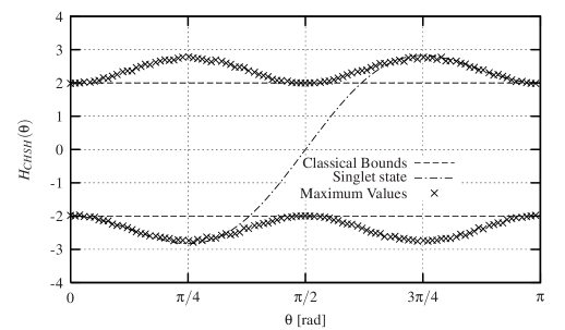
Figure 2: The quantum hull $H_{CHSH}$ as a function of a single parameter $\theta$.

II.2.2 CH case

Next we study the quantum hull corresponding to the CH inequality $-1\leq P_{CH}\leq 0$, with $P_{CH}=p_{13}+p_{14}+p_{24}-p_{23}-p_{1}-p_{4}$. As this inequality is essentially equivalent to the CHSH inequality discussed above if the expectation values are expressed by probabilities , we could in principle produce the same plot as in Figure 2 by the same choice of parameterization and a relabeling of the axes.

Again, the minmax principle yields the analytic expression for the hull; i.e.,

$$H_{CH}(\theta)={1\over 2}\left[\pm{\sqrt{3-\cos(2\theta)\over 2}}-1\right].$$ (4)

Thus, in terms of probabilities, the upper bound admitted by quantum mechanics is $H_{CH}(\theta)\leq(\sqrt{2}-1)/2$, corresponding to the Tsirelson bound of $2\sqrt{2}$ in the CHSH case.

To explore the quantum hull also for general configurations where the singlet state does not violate the inequality maximally, we restrict the projection operators $E_{i},\,F_{j}$ by ${E}_{1}(0)$, ${E}_{2}(\theta)={F}_{1}(\theta)$, ${F}_{2}(2\theta)$ to variations of one parameter $\theta$. In Figure 3 the quantum hull $H_{CH}$ of $P_{CH}$ obtained by substituting $p$ through $q$ is plotted along $0\leq\theta\leq\pi$. We can observe a maximum at $\theta=\pi/2$ that does not coincide with the maximum value reached by the singlet state.

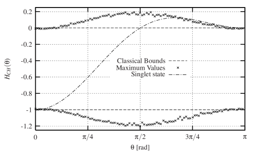
Figure 3: Quantum hull $H_{CH}$ as a function of a single parameter $\theta$.

II.2.3 Two particle three observable case

As a third example, consider a quantum hull associated with the configuration involving two spin 1/2 particles and three measurement directions. One of the 684 Bell-type inequalities enumerated in Pitowsky and Svozil (2001) is $-p_{14}+p_{15}+p_{16}+p_{24}+p_{26}+p_{34}+p_{35}-p_{36}\leq+p_{1}+p_{2}+p_{4}+p_{5}$. The associated quantum operator is given by

$$\begin{array}[]{l}O=-{E}_{1}\otimes{\mathbb{I}}-{E}_{2}\otimes{\mathbb{I}}-{\mathbb{I}}\otimes{F}_{1}-{\mathbb{I}}\otimes{F}_{2}-{E}_{1}\otimes{F}_{1}+{E}_{1}\otimes{F}_{2}+{E}_{1}\otimes{F}_{3}+\\ \qquad\qquad{E}_{2}\otimes{F}_{1}+{E}_{2}\otimes{F}_{3}+{E}_{3}\otimes{F}_{1}+{E}_{3}\otimes{F}_{2}-{E}_{3}\otimes{F}_{3}.\end{array}$$ (5)

Taking ${\rm tr}(WO)$ with a symmetric choice of measurement directions ${E}_{1}={F}_{1}=E(0)$, ${E}_{2}={F}_{2}=E(\theta)$, ${E}_{3}={F}_{3}=E(2\theta)$ ensures a violation of the inequality for the singlet state at $\theta=2\pi/3$ Pitowsky and Svozil (2001). The associated quantum hull $H_{O}$ is depicted in Figure 4.

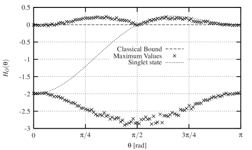
Figure 4: Quantum hull $H_{O}$ as a function of a single parameter $\theta$.

The three examples depicted in Figure 2-4 provide tests of the validity of quantum mechanics in the usual Bell-type inequality setup. They clearly exhibit a dependence of the quantum hull on the measurement directions; i.e., a particular set of projection operators determines the maximal possible violation of a Bell-type inequality, although the choice of a state is only restricted by fundamental quantum mechanical requirements.

II.3 Quantum Correlation Polytope

So far, we have considered certain quantum hulls associated with the faces of classical correlation polytopes, as well as bounds on expectation values, but we have not yet depicted the convex body $Q$ itself. In what follows, we shall get a view (albeit, due to the complexity of the contributions to $Q$, a not very sharp one) of the quantum correlation polytope for the two particle and two measurement directions per particle configuration. Note that classically, the corresponding CH polytope, denoted by $C(2)$, is bound by the $2^{4}$ vertices $(0,0,0,0,0,0,0,0)$, $(0,1,0,0,0,0,0,0),\ldots(1,1,1,1,1,1,1,1)$. These vertices are also elements of the quantum body $Q(2)$ consisting of vectors $(q_{1},q_{2},q_{3},q_{4},q_{13},q_{23},q_{14},q_{24})$ according to Eq. (I.2).

Consider a two-dimensional cut through the quantum body $Q(2)$ by restricting $q_{1}=q_{2}=q_{3}=a$ and $q_{13}=q_{14}=q_{24}=b$, $a,b\ \mbox{const.}$; i. e., by taking vectors of the form $(a,a,a,q_{4},b,q_{23},b,,b)$. These restrictions allow for a set of states $W$ and corresponding projection operators $E_{i},\,F_{j}$ such that six out of eight quantum probabilities have a definite value and the remaining probabilities $q_{4}$ and $q_{23}$ can vary within the quantum bounds. Numerically, after generating arbitrary states and arbitrary projection operators, a postselection is required for conformity to these restrictions. To find sufficiently many vectors, we specify the constants $a,b$ only up to a given tolerance value $\varepsilon$. More precisely, only states and projection operators yielding $q_{1}=q_{2}=q_{3}=a\pm\varepsilon$ and $q_{13}=q_{14}=q_{24}=b\pm\varepsilon$ for some $a,c$ are chosen.

We have set $a=1/2$, $b=3/8$, and the tolerance to $\varepsilon=\pm 0.015$. Note that this choice implicates the existence of vectors in $Q(2)$ which are outside $C(2)$, since the CH-inequality is violated for $q_{23}<1/8$ and $q_{4}=1/2$.

Figure 5 depicts a projection of the quantum body $Q(2)$ on the plane spanned by $q_{4}$ and $q_{23}$. Since the inequalities constituting the boundary lines have to be modified to account for $\varepsilon$, the size of $C(2)$ is enlarged to the dotted lines instead of the dashed lines indicating classical inequalities. Due to the non-uniform distribution of generated states, some regions are only sparsely populated. Nevertheless one can observe clearly points outside the classical polytope $C(2)$.

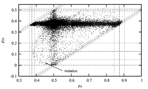
Figure 5: Cut through the quantum body $Q$ for $a=1/2$, $b=3/8$, $\varepsilon=\pm 0.015$.

We stress the importance of this first glance on $Q(2)$, since it constitutes the quantum analogy of the classical correlation polytope $C(2)$, which has been the basis of numerous experiments.

III Conclusion

Starting from the correlation polytopes which represent the restrictions of classical probabilities, we have used a general parameterization of quantum states and measurement operators to explore the quantum analogue. On the basis of the fundamental Bell-type inequalities, the quantum bounds have been visualized for specific configurations. We have presented a two-dimensional cut through an eight-dimensional quantum body clearly exhibiting regions of non-classical probability values.

The quantum bounds predicted in this article suggest experimental tests in at least two possible forms. First, our calculations provide an explicit way to construct quantum states, which, for the measurement setups associated with the orientation of Stern-Gerlach apparatus or polarizing beam splitters, yield maximal violations of the classical bounds by quantized systems. This is an extension of Tsirelson’s original findings Cirel’son (1980); Cirel’son (1993) (=Tsirelson). Based on the parametrization introduced above, Cabello has proposed such measurements Cabello (2003) with a suitable set of maximally entangled states. These bounds of quantum correlations have been experimentally tested and verified by Bovino et al. Bovino et al. (2003).

Apart from the concrete experiments mentioned above, there is a remote possibility of violations of the quantum bounds. At the moment, these speculations of stronger-than-quantum correlations Popescu and Rohrlich (1994); Mermin (1995); Krenn and Svozil (1998) appear hypothetical at best, since there is no theoretical indication that they may be realized physically (besides postselection schemes). The situation in this respect is clearly different from the classical bounds in Bell-type inequalities. Although Bell’s inequality does not compare classical probability theory with a specific theory either, an experimentalist can utilize these predictions because of the stronger-than-classical correlations of quantum mechanics. For instance, in the CHSH case, the experimenter chooses quantum mechanical setup and preparation procedures such that the quantum mechanical sum of correlations violates this bound most strongly. Stated pointedly, Bell’s inequality tells the experimentalist what to measure, but there is no empirical evidence supporting any experiment to trespass and falsify the quantum bounds. Nevertheless, it is interesting to know the quantum predictions exactly; not only from a principal or hypothetical point of view. Empirical implementations such as the Bovino et al. Bovino et al. (2003) experiment test the fine structure of the quantum limits beyond the Tsirelson bound.

This research has been supported by the Austrian Science Foundation (FWF), Project Nr. F1513.

References

- Boole (1958) G. Boole, An investigation of the laws of thought (Dover edition, New York, 1958).
- Boole (1862) G. Boole, Philosophical Transactions of the Royal Society of London 152, 225 (1862).
- Bell (1987) J. S. Bell, Speakable and Unspeakable in Quantum Mechanics (Cambridge University Press, Cambridge, 1987).
- Clauser and Shimony (1978) J. F. Clauser and A. Shimony, Rep. Prog. Phys. 41, 1881 (1978).
- Peres (1993) A. Peres, Quantum Theory: Concepts and Methods (Kluwer Academic Publishers, Dordrecht, 1993).
- Pitowsky (1986) I. Pitowsky, J. Math. Phys. 27, 1556 (1986).
- Pitowsky (1989a) I. Pitowsky, Quantum Probability—Quantum Logic (Springer, Berlin, 1989a).
- Pitowsky (1989b) I. Pitowsky, in Bell’s Theorem, Quantum Theory and the Conceptions of the Universe, edited by M. Kafatos (Kluwer, Dordrecht, 1989b), pp. 37–49.
- Pitowsky (1991) I. Pitowsky, Mathematical Programming 50, 395 (1991).
- Pitowsky (1994) I. Pitowsky, Brit. J. Phil. Sci. 45, 95 (1994).
- Froissart (1981) M. Froissart, Nuovo Cimento B 64, 241 (1981).
- Cirel’son (1980) B. S. Cirel’son, Letters in Mathematical Physics 4, 93 (1980).
- Cirel’son (1993) (=Tsirelson) B. S. Cirel’son (=Tsirelson), Hadronic Journal Supplement 8, 329 (1993).
- Ziegler (1994) G. M. Ziegler, Lectures on Polytopes (Springer, New York, 1994).
- Pitowsky and Svozil (2001) I. Pitowsky and K. Svozil, Physical Review A64, 014102 (2001), eprint quant-ph/0011060.
- Filipp and Svozil (2003) S. Filipp and K. Svozil, in Challenging the Boundaries of Symbolic Computation, Proceedings of the 5th International Mathematica Symposium, edited by P. Mitic, P. Ramsden, and J. Carne (Imperial College Press, London, 2003), pp. 215–222, eprint quant-ph/0105083.
- Garey and Johnson (1979) M. R. Garey and D. S. Johnson, Computers and Intractability. A Guide to the Theory of NP-Completeness (Freeman, San Francisco, 1979).
- Popescu and Rohrlich (1994) S. Popescu and D. Rohrlich, Foundations of Physics 24, 379 (1994).
- Krenn and Svozil (1998) G. Krenn and K. Svozil, Foundations of Physics 28, 971 (1998).
- Mermin (1995) D. N. Mermin, Annals of the New York Academy of Sciences 755, 616 (1995).
- Khalfin and Tsirelson (1992) L. A. Khalfin and B. S. Tsirelson, Foundations of Physics 22, 879 (1992).
- Pitowsky (2002) I. Pitowsky, in Quantum Theory: Reconsideration of Foundations, Proceeding of the 2001 Vaxjo Conference, edited by A. Khrennikov (World Scientific, Singapore, 2002), eprint quant-ph/0112068.
- Halmos (1974) P. R. Halmos, Finite-dimensional vector spaces (Springer, New York, Heidelberg, Berlin, 1974).
- Werner and Wolf (2001) R. F. Werner and M. M. Wolf, Phys. Rev. A 64, 032112 (2001), eprint quant-ph/0102024, URL http://link.aps.org/abstract/PRA/v64/e032112.
- Cabello (2003) A. Cabello (2003), eprint quant-ph/0309172.
- Fishburn and Reeds (1994) P. C. Fishburn and J. A. Reeds, SIAM J. Disc. Math. 7, 48 (1994).
- Cabello (2002a) A. Cabello, Physical Review Letters 88, 060403 (2002a), eprint quant-ph/0108084.
- Cabello (2002b) A. Cabello, Physical Review A 66, 042114 (2002b), eprint quant-ph/0205183.
- Bovino et al. (2003) F. A. Bovino, G. Castagnoli, S. Castelletto, I. P. Degiovanni, M. L. Rastello, and I. R. Berchera (2003), eprint quant-ph/0310042.
- Cereceda (2001) J. L. Cereceda, Foundations of Physics Letters 14, 401 (2001), eprint quant-ph/0101143.