Quantum Dynamics of Magnetic and Electric Dipoles and Berry’s Phase

Abstract

We study the quantum dynamics of neutral particle that posseses a permanent magnetic and electric dipole moments in the presence of an electromagnetic field. The analysis of this dynamics demonstrates the appearance of a quantum phase that combines the Aharonov-Casher effect and the He-Mckellar-Wilkens effect. We demonstrate that this phase is a special case of the Berry’s quantum phase. A series of field configurations where this phase would be found are presented. A generalized Casella-type effect is found in one these configurations. A physical scenario for the quantum phase in an interferometric experiment is proposed.

In 1959 Aharonov and Bohm (AB)aha demonstrated that a quantum charge circulating a magnetic flux tube acquire a quantum topological phase. This effect was observed experimentally by Chambersprl:cham ; pes . Aharonov and Casher(AC) showed that a particle with a magnetic moment moving in an electric field accumulates a quantum phase, the AC phasecas . This phenomenon has been observed in a neutron interferometercim and in a neutral atomic Ramsey interferometersan ; san1 .

He and McKellarmac , and Wilkenswil , independently, have predicted the existence of a quantum phase that an electric dipole acquires, while circulating around, and parallel to a line of magnetic monopoles. This phase has been denominated in the literature the He-McKellar-Wilkens(HMW) phase, and it is the Maxwell dual of AC phase. A simple practical experimental configuration to test the HMW phase, was proposed by Wei, Han and Weiwei where the electric field of a charged wire polarizes a neutral atom and an uniform magnetic field is applied parallel to the wire. In this field configuration, the atom acquires a HMW phase. Dowling, Williams and Fransonfra have proposed a unified description of all three phenomena(AB, AC, HMW phase) discussing Maxwell electromagnetic duality relation between the three quantum phases. The analysis of the duality predicts a fourth phenomenon, which is the dual of Aharonov-Bohm effect(dAB). In a recent article Anandanana has presented a unified and fully relativistic treatment of the interaction between a particle with permanent electric and magnetic dipole moments and an electromagnetic field. This phase we designate Anandan topological phase.

In the early eighties Berry discovered ber that a slowly evolving(adiabatic) quantum system retains information of its evolution when returnes to its original physical state. This information corresponds to what is termed Berry’s phase. The appearance of this phase has been generalized to the case of non-adiabatic ahan evolution of a quantum system. In any case the phase only depends on the geometrical nature of the pathway along which the system evolves. This phenomenon has been investigated in several areas of physics. There are various experiments which have been reported concerning the appearance of the adiabatic and non-adiabatic geometric phases, including the observations on photonstom , neutronsbit and nuclear spinstyc . The manifestations of Berry’s quantum phase in high-energy electron diffraction in a deformed crystal, which contains a screw dislocation, has also been observed bir . The quantum evolution of a single particle is given by a time-dependent Schrödinger equation $i\frac{d}{dt}|\psi(t)\rangle=\mathcal{H}(R_{i}(t))|\psi(t)\rangle,$ where $H(R_{i}(t))$ is the system Hamiltonian which depends on a set of externally controllable parameters ${\bf R}(t)=R_{i}$. The solution of the Schrödinger equation in the adiabatic approximation is given by $|\psi(t)\rangle=\exp[-i\int_{0}^{t}{\cal E}(t)dt]\exp(i\gamma(C))|\psi({\bf R}(t))\rangle,$ where $|\psi({\bf R}(t))\rangle$ are instantaneous eigenstates of the Hamiltonian with eigenvalues ${\cal E}(t)$. The first factor of the phase is the usual dynamical one. The extra phase factor, $\exp(i\gamma(C))$, becomes physically important when the parameters are changed along a path $C$ in the parameter space, over some time $T$, such as $R(T)=R(0)$. The non-trivial phase factor is Berry’s phase for the path $C$ which is given by $\gamma_{n}(C)=i\oint_{C}\langle\psi({\bf R})|\nabla_{R}\psi({\bf R})\rangle d{\bf R},$ where the term $\langle\psi({\bf R})|\nabla_{{\bf R}}\psi({\bf R})\rangle$ is denominated Berry connection. Berry showed that the AB-effect is a special case of this geometrical phase. In 1991, Mignanimig and He and McKellarmac1 also demonstrated by a different approach that the AC-phase is a particular case of Berry’s quantum phase.

In this rapid communication we analyze Anandan’s phase for a quantum particle with permanent magnetic and electric dipole moments in a radial configuration of electric and magnetic fields and we study the appearance of a geometrical quantum phase in their dynamics. We also demonstrate that Anandan’s topological phase is a special case of the Berry’s geometrical phase.

We consider now the situation pointed by Anandan of a neutral particle with permanent electric ($\mathbf{d}$) and magnetic (${\bm{\mu}}$) dipole moments. The non-relativistic Lagrangian ($c=1$) that describes this particle in the presence of an electromagnetic field is given by

$$\mathcal{L}=\frac{1}{2}mV^{2}+\mathbf{d}\cdot(\mathbf{E}+\mathbf{V}\times\mathbf{B})+\bm{\mu}\cdot(\mathbf{B}-\mathbf{V}\times\mathbf{E})$$ (1)

From (1) we obtain the canonical momentum,

$$\mathbf{P}=m\mathbf{V}-\bm{\mu}\times\mathbf{E}+\mathbf{d}\times\mathbf{B},$$ (2)

and the equation of motion for the particle is given by

$$m\ddot{\mathbf{r}}=\bm{\nabla}(\mathbf{\mu}\cdot\mathbf{B} + \mathbf{d}\cdot\mathbf{E})+\bm{\mu}\times\frac{\partial\mathbf{E}}{\partial t}-\mathbf{d}\times\frac{\partial\mathbf{B}}{\partial t}+\mathbf{V}\cdot\bm{\nabla}(\bm{\mu}\times\mathbf{E})-\mathbf{V}\cdot\bm{\nabla}(\mathbf{d}\times\mathbf{B})-\bm{\nabla}(\bm{\mu}\cdot\mathbf{V}\times\mathbf{E})$$

$$+ \bm{\nabla}(\mathbf{d}\cdot\mathbf{V}\times\mathbf{B})-\mathbf{\dot{d}}\times\mathbf{B}+\mathbf{\dot{\mu}}\times\mathbf{E}$$

We use $\frac{d}{dt}=\partial_{t}+\mathbf{v}\cdot\bm{\nabla}$ and the Maxwell equations $\partial_{t}\mathbf{B}=-\bm{\nabla}\times\mathbf{E}$ and $\partial_{t}\mathbf{E}=\bm{\nabla}\times\mathbf{B}$. We also use the identities $\bm{\nabla}(\mathbf{d}\cdot\mathbf{E})=(\mathbf{d}\cdot\bm{\nabla})\mathbf{E}+\mathbf{d}\times(\bm{\nabla}\times\mathbf{E})$ and the similar one for the magnetic case. After some mathematical manipulation, equation (Quantum Dynamics of Magnetic and Electric Dipoles and Berry’s Phase) assumes the following form

$$m\ddot{\mathbf{r}} = (\mathbf{d}\cdot\bm{\nabla})\mathbf{E}-\mathbf{v}\times\bm{\nabla}\times(\mathbf{d}\times\mathbf{B})+\dot{\mathbf{d}}\times\mathbf{B}$$ (4)

$$+ (\bm{\mu}\cdot\bm{\nabla})\mathbf{B}+\mathbf{v}\times\bm{\nabla}\times(\bm{\mu}\times\mathbf{E})-\dot{\bm{\mu}}\times\mathbf{E}.$$

For a complete description of the dynamics of this particle we need to find the equation that describes the dynamics of dipoles. We assume that $\mathbf{d}$ and $\bm{\mu}$ refers to a permanent electric and magnetic dipoles of a molecule or atom, respectively. Hence, with the proviso of a subsequent justification, we set $\dot{\mathbf{d}}=0$ and $\dot{\bm{\mu}}=0$, in Eq. (4), and we consider that laboratory fields $\mathbf{E}$ and $\mathbf{B}$ do not vary in the dipole directions, and therefore $(\vec{d}\cdot\bm{\nabla})\mathbf{E}=0$ and $(\bm{\mu}\cdot\bm{\nabla})\mathbf{B}=0$. In this paper we do not consider the new contribution for the topological phase found by Spavieri spa , since his contributions were null due to the field configurations adopted in this work. In this way, the equation of motion is given by

$$m\ddot{\mathbf{r}}=\mathbf{v}\times\bm{\nabla}\times[\bm{\mu}\times\mathbf{E}-\mathbf{d}\times\mathbf{B}].$$ (5)

This force is reminiscent of the force experienced by an electron moving in a magnetic field $e^{-1}\bm{\nabla}\times[\bm{\mu}\times\mathbf{E}-\mathbf{d}\times\mathbf{B}]$. The non-relativistic Hamiltonian for this problem can be obtained from the Lagrangian, and is given by

$$\hat{\mathcal{H}}=\frac{1}{2m}(\hat{\mathbf{p}}-{\bm{\mu}}\times{\bf E}+{\bf d}\times{\bf B})^{2}-{\bm{\mu}}\cdot{\bf B}-{\bf d}\cdot{\bf E}.$$ (6)

Let us analyze the quantum dynamics of a particle governed by the Hamiltonian(6). In the region in which the particle is immersed, we consider that the fields are cylindrically radial. We adopt the following generic fields

$$\mathbf{B}=\frac{\lambda_{m}}{\rho}\hat{e_{\rho}}\quad\mathbf{E}=\frac{\lambda_{e}}{\rho}\hat{e_{\rho}},$$ (7)

where $\lambda_{m}$ is a constant that depends on the array of magnetic dipoles or magnetic charges that generate a magnetic field and $\lambda_{e}$ is an electric charge density that creates the electric field. With this field configurations the expression for the force experienced by the particle, (Eq.(5)) is null. If we analyze the expression for the torque experienced by the dipoles in this field arrangement we can see that it vanishes. In this way the conditions for the existence of topological phase can be assuredana . The potential term in the Hamiltonian (6) gives null contribution to the dynamics of this dipole in the field configurations (7) if the dipoles are prepared to be aligned with the $z$-direction. We assume that the particle is moving in the $x-y$ plane , in an external electric and magnetic field. We also suppose that the fields generated by the sources are radially distributed in the space. We adopt a treatment analogous to the Aharonov-Bohm effect as used by Berryber . In this framework, Berry’s phase can be calculated by use of the following arguments: let us confine the quantum system to a perfectly reflecting box such that the wave packet is nonzero only in the interior of the box. The vector that localizes the box in relation to the source of electromagnetic field is called ${\bf R}$. This vector is oriented from the origin of the coordinate system (localized on the source) to the center of the box. In the absence of fields, the wave function for the particle in the box is given by $\psi_{0}({\bf r}-{\bf R})$ where ${\bf r}$ represents the coordinates of the particle centered at R. We use the Dirac phase factor method to describe the quantum dynamics of the particle. In this approach the quantum state of the particle in the presence of these electromagnetic fields can be written as a function of the quantum state in the absence of the electromagnetic field times a multiplicative exponential term that depends on the fields. The quantum dynamics is governed by the time-dependent Schrödinger equation, and the quantum state can be written as

$$|\Psi(t)\rangle=\exp\left[-i\int_{0}^{t}{\cal E}(t)dt\right]\times$$

$$\exp\left[-i\int_{R}^{r^{\prime}}(\bf{d}\times\bf{B}-\bm{\mu}\times\bf{E})dr^{\prime}\right]|\Psi_{0}({\bf R}(t))\rangle,$$ (8)

where $|\psi_{0}(\rho,\phi)\rangle$ is the solution of the Schrödinger equation in absence of fields. The first term in (Quantum Dynamics of Magnetic and Electric Dipoles and Berry’s Phase) is the dynamical phase and the second one is the Berry’s geometrical phase. If we transport the box around the sources of the electromagnetic fields, the wave function of the particle acquires a Berry’s quantum phase. Then, in order to compute this, we need to calculate the Berry’s connections

$$A_{ij} = \langle\Psi({\bf r}-{\bf R})|\nabla_{\bf{R}}(\Psi({\bf r}-{\bf R})\rangle=\int d^{3}{\bf r}\Psi^{*}(\bf{r}-\bf{R})[-i(\bf{d}\times\bf{B}-\bm{\mu}\times\bf{E})\Psi(\bf{r}-\bf{R})+\nabla_{\bf{R}}\Psi(\bf{r}-\bf{R})].$$ (9)

Which results in

$$A_{ij}=i(\bf{d}\times\bf{B}-\bm{\mu}\times\bf{E}).$$ (10)

Thus, the Berry’s phase is given by

$$\gamma_{c}(C)=\oint(\bf{d}\times\bf{B}-\bm{\mu}\times\bf{E})d\bf{R}.$$ (11)

The effect is observed as an interference between the particle in the transported box and one in a box which was not transported around the circuit. This result demonstrates the existence of Berry’s quantum phase in the dynamics of a neutral particle that contains a permanent electric and magnetic moments of dipole. Our purpose at this moment is to introduce some setups in which we obtain certain field and dipole moment configurations where this phase can be observed.

The first set-up that we analyze is the radial field configuration presented in (7). The arrangement of field configurations with the magnetic field radially cylindrical is more difficult to achieve experimentally, due to the fact that, a priori, we need a linear distribution of magnetic charges. We can observe in the literature that this kind of arrangement would be possible. Some authors have claimed that this configuration can be obtained experimentally as in the arrangements presented in the articlesmag ; mag1 ; mag2 . In this experimental set, the radial magnetic field is produced by two concentric cylindrical magnets, and in this way a radial magnetic field can be produced between the magnets. More realistic configuration that can generate a radial magnetic field is when we consider a cylindrical solenoid carrying a surface current density that produces, in the external region of a solenoid, a field configuration with the same characteristics of (7) chys . Despite all difficulties to do a real experiment, we suppose that it is possible. If we cogitate in this region the existence of a radial electric field generated by an internal cylindrical electrode, we verify that Berry’s quantum phase (11) has the following expression

$$\gamma_{c}(C)=2\pi\mu\lambda_{e}-2\pi d\lambda_{m}.$$ (12)

Other device of radial magnetic and electric fields is obtained if we use the same arguments presented by Tkachuk tka . In that case, he has considered that the radial field configurations are generated by a charged ferromagnetic wire in the $z$-direction. We use this arrangement with a simple difference, namely we adopt here that the ferromagnetic wire is electrically charged. The magnetization is parallel to the wire and its magnitude is $M(z)=-\lambda_{m}z$, where $\lambda_{m}$ can be treated as a linear magnetic charge density. Additionally this wire has a linear electric charge density that generates a radial electric field. When the wire is sufficiently long, the magnetic and electric fields around the central part of the wire are

$${\bf B}=\frac{2\lambda_{m}}{\rho}\hat{e_{\rho}}\quad{\bf E}=\frac{\lambda}{\rho}\hat{e_{\rho}}.$$ (13)

Berry’s quantum phase (11) for the modified Tkachuk’s configuration is given by the following phase factor

$$\gamma_{c}(C)=2\pi\mu\lambda_{e}-4\pi d\lambda_{m}.$$ (14)

For the field configurations analyzed in the present letter we observe that: for the case $\lambda_{e}=0$, obtained from Eq.(11), the HMW phase is a special case of Berry’s phase. In the case $\lambda_{m}=0$, the results of Mignanimig and He and McKellarmac for the Aharonov-Casher effects are obtained. In the case $\lambda_{e}\neq 0$ and $\lambda_{m}\neq 0$, we obtain Anandan’s generalized topological phase for a quantum particle (atom or molecule), with a permanent magnetic and electric dipole moments. This is a special case of the geometric Berry’s quantum phase.

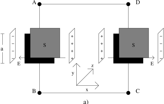
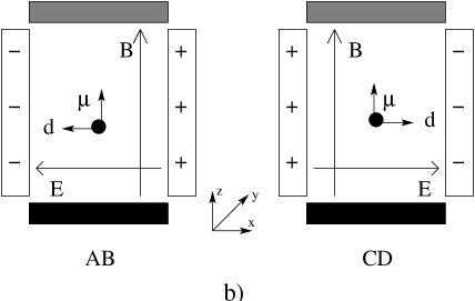
Figure 1: a)Schematic diagram for obtaining Anandan’s phase. We assume that beam of particles are prepared with magnetic moment aligned with thez-direction and are introduced in a region with velocity in y-direction, where a constant magnetic field is also present in the z-direction. We also have a electric field in x-direction. b)Cross section where we can see the dipole alignments.

Now, the analysis of the Berry’s phase in this system is developed in the following way: we are interested in finding configurations of d, $\bm{\mu}$, B and E that make the classical torque and force to vanish. Recently Leelee has studied the quantum phase in dynamics of the electric or magnetic dipoles and he observes that it is possible to write a vector potential for magnetic or electric dipole using the point of view of the Aharonov Bohm effect, noting that there is a dual effect of the Casellacase effect for dipole. The setup introduced by Lee, has guided our third configuration for a very simple apparatus for observation of the quantum phase in the present case. We can find that the electric dipole, in this apparatus, is orthogonal to B and v at the same time. In the same way if the magnetic dipole is perpendicular to E and v, it has the property of vanishing both, torque and force. The quantum phase acquired by both dipoles is only independent of the trajectory in opposition to the Aharonov-Bohm phase that is independent of the trajectory and is also independent of the solenoid configuration. The trajectory of the dipoles is restricted and the velocity should be perpendicular to both moments because of the relativistic effects in the fields. We consider a schematic experiment showed in figure(1). We assume that a beam of atoms or molecules, with permanent magnetic dipole moments and that can induces electric dipole moments in it, is prepared with the magnetic dipole moment aligned with z-direction and the electric dipole moment aligned with x-direction. This beam is introduced in the interferometer device with a set of two dipole magnets with the magnetic field in z-direction and two generators of uniform electric field in x-direction but in opposite direction as showed in figure (1). The resultant phase acquired by atoms (or molecules) in this interferometer paths is given by

$$\gamma(c)=2dB_{0}a+2\mu E_{0}a$$ (15)

where $B_{0}$ and $E_{0}$ are the magnitude of the fields in both path around the apparatus and $a$ is the length of both, magnets and electric plates. For $E_{0}=0$ we have the dual Casella effect predicted by Lee; for $B_{0}=0$ we have the Casella effect. This is a generalized Casella effect and also is a case of the Anandan phase.

We have shown that the Anandan quantum phase is a special case of Berry’s phase. Our purpose is to configure a process similar to an interferometer to try to observe this quantum phase. If we can be able to do it, we hope that neither a classical force nor a classical torque will act in the test particle(which can be an atom or molecule). The interference framework should be explained only by a quantum potential effect in the sense of the Aharanov-Bohm effect. We have demonstrated three configurations where the geometric phase can be detected. In the third configuration we have obtained a generalized Casella effect that is a case of a class of phases treated in this work.

- (1) Y. Aharonov and D. Bohm, Phys. Rev. 115, 485 (1959).
- (2) R. G. Chambers, Phys. Rev. Lett. 5,3 (1960).
- (3) M. Peshkin and A. Tonomura, The Aharonov-Bohm Effect (Springer-Verlag, Berlin, 1989).
- (4) Y Aharonov and A. Casher, Phys. Rev. Lett. 53, 319, (1984).
- (5) A. Cimmino et al., Phys. Rev. Lett. 63, 380 (1989).
- (6) K. Sangster et al., Phys. Rev. Lett. 71,3641 (1993).
- (7) K. Sangster et al., Phys. Rev. A 51, 1776 (1995).
- (8) X. -G. He and B. H. J. McKellar, Phys. Rev. A, 47, 3424 (1993).
- (9) M. Wilkens, Phys. Rev. Lett. 72, 5 (1994).
- (10) H. Wei, R. Han and X. Wei, Phys. Rev. Lett. 75, 2071 (1995).
- (11) J. P. Dowling, C. P. Williams and J. D. Franson, Phys. Rev. Lett. 83, 2486(1999).
- (12) J. Anandan, Phys. Rev. Lett. 85, 1354 (2000).
- (13) M. V. Berry, Proc. R. Soc. London, A 392, 457 (1984).
- (14) Y. Aharonov and J. Anandan, Phys. Rev. Lett. 58, 1593 (1987).
- (15) A. Tomita and R. Y. Chiao, Phys. Rev. Lett. 57, 937 (1986) ; R. Simon, H. J. Kimble and E. C. G. Sudarshan, Phys. Rev. Lett. 61, 19 (1988)
- (16) T. Bitter and D. Dubbers, Phys. Rev. Lett. 59, 251 (1987) .
- (17) R. Tycko, Phys. Rev. Lett. 58, 2281 (1987).
- (18) D. M. Bird and A. R. Preston, Phys. Rev. Lett. 61, 2863 (1988).
- (19) R. Mignani, J. Phys. A: Math. Gen. 24, L421 (1991).
- (20) X. -G. He and B. H. J. McKellar, Phys. Lett. B 264 129 (1991)
- (21) G. Spavieri, Phys. Rev. Lett. 82, 3932 (1999).
- (22) W. H. Heiser and J. A. Shercliff, J. Fluid Mech. 22, 701 (1985).
- (23) S. Y. Molokov and J. E. Allen, J. Phys. D: Appl. Phys. 25, 393 (1992).
- (24) S. Y. Molokov and J. E. Allen, J. Phys. D: Appl. Phys. 25, 933 (1992).
- (25) C. Chyssomalakos, A. Franco and A. Reyes-Coronado, “Spin particle on a Cylinder with Radial Magnetic Field”, quant-ph/0212054 (2002).
- (26) V. M. Tkachuk, Phys. Rev. A 62, 052112 (2000).
- (27) T. -Y. Lee, Phys. Rev. A 64 032107 (2001).
- (28) R. C. Casella, Phys. Rev. Lett. 65, 221 (1990).