Quantum Computing with Atomic Josephson Junction Arrays

Abstract

We present a quantum computing scheme with atomic Josephson junction arrays. The system consists of a small number of atoms with three internal states and trapped in a far-off resonant optical lattice. Raman lasers provide the “Josephson” tunneling, and the collision interaction between atoms represent the “capacitive” couplings between the modes. The qubit states are collective states of the atoms with opposite persistent currents. This system is closely analogous to the superconducting flux qubit. Single qubit quantum logic gates are performed by modulating the Raman couplings, while two-qubit gates result from a tunnel coupling between neighboring wells. Readout is achieved by tuning the Raman coupling adiabatically between the Josephson regime to the Rabi regime, followed by a detection of atoms in internal electronic states. Decoherence mechanisms are studied in detail promising a high ratio between the decoherence time and the gate operation time.

I Introduction

Josephson effects originate from a tunneling of the particles in the condensed modes between two superfluids and reflect the phase difference of the macroscopic wave functions between the superfluids. Initially discovered in the superconductors [1, 2], Josephson effects have been studied intensively in trapped atoms both theoretically and experimentally [3, 4]. In the atomic case, Josephson junctions can be constructed between two superfluids spatially separated by a double well potential and can be constructed between atomic internal modes coupled by lasers. Studies include the macroscopic quantum coherence between two atomic condensates and the observation of the Josephson dynamics. [5]

One important application of the Josephson junctions discussed in recent years is in quantum computing. Various superconducting Josephson devices have been proposed for implementing a quantum computer, including the charge qubit, the flux qubit, the phase qubit. These qubits have been experimentally tested and have shown quantum coherent oscillations between macroscopically distinguishable states[6, 7, 8].

The atomic Josephson junctions can also be explored for quantum computing. In this paper, we present a candidate for implementing an atomic “flux” qubit with small number of atoms in an optical trap. We assume that a Bose Einstein condensate with three atomic states is stored in the lowest vibrational state of an optical trap[9]. The three internal atomic states correspond to three bosonic modes. Each mode is the analogue of a superconducting metallic island. Raman lasers generate the Josephson links between the internal modes, while atomic collisions provide an effective capacitive couplings between the modes. The phase differences between lasers plays the role of the magnetic field in the superconducting loop. With the competition between the Josephson energy and the collision energy, the atoms behave collectively and the stationary states of the qubit have a coherent particle transfer –the persistent current – between the internal modes. With only $15$ atoms[10], the atomic counterpart of the superconducting flux qubit[7, 8] can be realized, which bears all the qualitative features of the superconducting flux qubit.

Compared with the superconducting flux qubit, the parameters of the atomic “flux” qubit can be controlled with large flexibility and high uniformity. Both the Josephson coupling and the collision interaction can be adjusted by external electro-magnetic sources. The Josephson couplings of different junctions can be made to high accuracy with the fine control of laser. While for superconductors, not only that the junction parameters fluctuate due to the inaccuracy in fabrication, but the parameters are fixed for one sample. This advantage makes it easier to scale up the number of qubits in the atomic systems and provides various ways to implement gate operations. Another merit of the atomic qubit is that a projective measurement can be performed by adiabatically switching the Raman couplings. On the contrary, an efficient readout for the solid-state qubits is a problem many people are studying. The drawback of the atomic qubit is the slow gate speed which is limited by the strength of the collision interaction. Meanwhile, this drawback can be compensated by the long decoherence time. In the solid-state systems, various elementary excitations can damage the coherence of the quantum states in a time that is only one order longer than the gate time; while we show that in the atomic qubit, the decoherence time is thousand times of the gate operation time.

In the following, the major results are summarized. In section II, we briefly review the superconducting flux qubit and the experimental achievement for the flux qubit. In section III, we give a detailed description of our proposal for the atomic “flux” qubit and how it can be realized experimentally. We also characterize the qubit at different parameter regimes and present typical energy scales for the qubit. In section IV, we introduce the phase mode to compare this qubit with the superconducting one and show that a small number of atoms indeed represents the macroscopic behavior of a Josephson junction. This section is followed by section V where the implementation of quantum logic gates are studied. In section VI, a quantum nondemolition measurement scheme is constructed via the adiabatic switching of the Josephson couplings. The decoherence of the qubit is discussed in section VII. The conclusions are given in section VIII.

II The superconducting flux qubit

Josephson junctions have been proved to be a promising building block for quantum computers. Various proposals of Josephson circuits at different parameter regimes have been studied[6, 7, 8]. Among these, the superconducting flux qubit—also named the persistent-current qubit—has been intensively studied both theoretically and experimentally. In the following, we briefly summarize the basic facts of the flux qubit in superconducting Josephson Junctions, to allow comparison with the atomic “flux” qubit introduced in the following section.

A The Circuit of the Qubit

The superconducting flux qubit[7, 8] is a superconducting loop with three Josephson junctions in series, as in Fig. 1a. Written in terms of the phase differences cross the bottom two junctions, $\varphi_{1}$ and $\varphi_{2}$, the Hamiltonian (Eq. (11) in [8]) is

$${\cal H}_{t} = \frac{1}{2}\vec{P}^{T}{\bf M}^{-1}\vec{P}+E_{J}\{2+\alpha-\cos\varphi_{1}-\cos\varphi_{2}$$ (2)

$$-\alpha\cos(2\pi f_{1}+\varphi_{1}-\varphi_{2})\}$$

where $\vec{P}=(\hat{P}_{1},\hat{P}_{2})^{T}$ are the conjugates of the phase variables and have the physical meaning of the charges on the islands. The first term is the capacitive energy with ${\bf M}=(\hbar/2e)^{2}{\bf C}$ where ${\bf C}$ is the capacitance matrix of the circuit. The rest of the terms are the Josephson energy with $E_{J}=I_{c}(\frac{\hbar}{2e})^{2}$ and $I_{c}$ being the critical current of the junctions. The third junction at the top of the circuit has a Josephson energy of $\alpha E_{J}$ with $\alpha=0.75$. The magnetic flux in the loop, $f_{1}$ in unit of the flux quantum $\Phi_{0}=\hbar/2e$, is an important control parameter for the qubit. Both the stationary states and the one-bit logic gates are controlled via this flux.

The Hamiltonian in Eq. (2) describes a phase particle in a two-dimensional periodic potential as is shown in Fig. 1b. Each unit cell has two energy minima and is a double well potential. At $f_{1}=0.495$, the lowest two states of the qubit localize in one of the two wells respectively and have opposite circulating currents. At $f_{1}=1/2$, the lowest two states are symmetric and antisymmetric superpositions of the localized flux states and the energy splitting is due to the tunneling of the flux states over the potential barrier. Considering only the lowest states, the qubit can be described by the Pauli matrices for a $1/2$ spin: ${\cal H}_{q}=\frac{\epsilon_{0}}{2}\sigma_{z}+\frac{t_{0}}{2}\sigma_{x}$, where the eigenstates of $\sigma_{z}$ are the localized flux states and $\epsilon_{0}$ varies linearly with $(f_{1}-1/2$). Typically, the Josephson energy is $E_{J}=200\,{\rm GHz}$ and $E_{J}/E_{C}=80$. Numerical calculations of the energy and current are shown in Fig. 1c. The energy difference of the qubit states at $f_{1}=0.495$ is $\omega_{q}\sim 10\,{\rm GHz}$ with the average currents of $\pm 0.7I_{c}$; at $f_{1}=1/2$, $t_{0}=10\,{\rm GHz}$.

For a quantum circuit to be a good qubit for fault-tolerant quantum computing, five requirements have to be met[12]: 1. to identify a scalable quantum system; 2. to perform universal quantum logic gates; 3. to prepare the initial state; 4. to read out the qubit states; 5. to have a decoherence time longer than $10^{4}$ quantum operations. The three-junction loop behaves as an effective two-level system and can be mapped onto a $1/2$-spin. The qubit can be prepared to the ground state by cooling it to a temperature of $T\sim 50\,{\rm mK}\ll\omega_{q}$.

B Quantum Logic Gates

To achieve universal quantum logic operations, two elementary gates are required: single qubit rotation and two qubit controlled gate. For the superconducting flux qubit, the single qubit gate is by applying microwave oscillations to the superconducting loop. Typically, the Rabi frequency is $\omega_{r}=10-100\,{\rm MHz}$ in proportional to the amplitude of the microwave. The two qubit gate is constructed via the coupling of the circulating currents of the two qubits: ${\cal H}_{int}=M_{12}|\langle I_{1}\rangle\langle I_{2}\rangle|$ with $I_{1,2}$ being the currents of the two qubits and $M_{12}$ being the mutual inductance. The interaction can be of order of $1\,{\rm GHz}$.

C Qubit State Readout

The qubit is measured by inductively coupling the qubit to a dc SQUID magnetometer which is a superconducting loop with two Josephson junctions as is shown in Fig. 1d. When the current that flows through the SQUID increases, the SQUID stays in the superconducting state until a critical current $I_{c}^{eff}$ where the SQUID makes a transition to a finite voltage state. The critical current is varied by the flux generated by the qubit: $\delta I_{c}^{eff}=\pm\delta\varphi_{q}I_{c}^{sq}\sin\pi f_{ex}$ where $f_{ex}$ is the external flux in the SQUID and $\pm\delta\varphi_{q}$ are flux of the two qubit states respectively. By measuring the critical current, the qubit states are read out. Due to fluctuations, the measured critical current has a distribution that is wider than $\delta I_{c}^{eff}$ which results in a nonprojective measurement of the qubit.

D Decoherence

Many factors can result in quantum errors against the superconducting qubits. First, the errors can come from the imperfect control of the qubit circuits, for example, off-resonant transitions during gate operations and unwanted dipolar couplings between qubits. These errors can be prevented by the quantum control approach. Second, the fluctuations of the environment of qubit can cause decoherence of the qubit. In the solid-state qubits, many elementary excitations exist that can damage the qubit state, including the dipolar interactions between the qubit and the nuclear spins, the background charge fluctuations, and the noise coupled to the qubit from the measurement circuits. The decoherence time measured in experiments is $100\,{\rm nsec}$[11] which is about $10$ times of the operation time. This gives a lower bound for the generic decoherence of the qubit.

III The Atomic “flux” Qubit

In this section we present an atomic counterpart of the superconducting flux qubit. The qubit is made of a mesoscopic Bose Einstein condensate of three-level atoms trapped in the lowest motional states of an optical trap, and interacting with each other via cold collision. Josephson junctions, which are the building block of this qubit, are constructed by laser coupling of the three bosonic modes of the trapped atoms.

A The Physical System and the Hamiltonian

We consider a small number of three-level atoms trapped in a 1D optical lattice, as is shown in Fig. 2a, which is described by the Hamiltonian

$${\cal H}_{0} = \displaystyle\sum_{\alpha}\int d\vec{x}\,\psi_{\alpha}^{\dagger}(\vec{x})\left(-\frac{\bigtriangledown^{2}}{2M}+V(\vec{x})\right)\psi_{\alpha}(\vec{x})$$ (3)

$$+ \displaystyle\sum_{\alpha,\beta}U_{\alpha\beta\alpha^{\prime}\beta^{\prime}}\int d\vec{x}d\vec{x}^{\prime}\,\psi_{\alpha}^{\dagger}(\vec{x})\psi_{\beta}^{\dagger}(\vec{x}^{\prime})\psi_{\beta}^{\prime}(\vec{x}^{\prime})\psi_{\alpha}^{\prime}(\vec{x})$$ (4)

$$+ \displaystyle\sum_{\alpha\neq\beta}\int d\vec{x}\,\left(\Omega_{\alpha\beta}(\vec{x})\psi_{\alpha}^{\dagger}(\vec{x})\psi_{\beta}(\vec{x})+h.c\right),$$ (5)

where the three internal states are labeled by $\alpha,\beta$. The first term is the single particle energy in a harmonic trapping potential: $V(\vec{x})=\frac{1}{2}m\omega_{\parallel}^{2}x^{2}+\frac{1}{2}m\omega_{\perp}^{2}(y^{2}+z^{2})$, where $\omega_{\perp,\parallel}$ are the trapping frequencies in the transversal direction and the longitudinal direction respectively. With a cigar-shaped geometry, we have $\omega_{\perp}\gg\omega_{\parallel}$. We assume that the trapping frequencies are much larger than all other relevant time scales (e.g. the qubit energy and the gate speed) so that the atoms stay in the motional ground states and the qubit can be described by a three-mode Hamiltonian. The second term in Eq. (5) is the collision interaction. In practice, this term can be more complicated due to the scattering between the atoms in different internal states: for example, in the case of a hyperfine $F=1$, $M_{F}=0,\pm 1$ there will be collisional terms where two atoms in state $M_{F}=0$ collide to produce an atom in states $M_{F}=+1$ and $-1$ states. These terms can be suppressed by shifting the atomic levels by external fields, so that energy conservation in the collision is violated, i.e. these terms average away in the Hamiltonian. Furthermore, detailed numerical studies show (see below) that we can simplify the collisional term to a fully symmetric interaction with $U_{\alpha\beta\alpha^{\prime}\beta^{\prime}}=\delta_{\alpha\beta}\delta_{\alpha\alpha^{\prime}}\delta_{\beta\beta^{\prime}}U_{0}$, the main physical properties of the qubit are well preserved. Here, the interaction strength is

$$U_{0}=\displaystyle\frac{4\pi\hbar^{2}a_{s}}{m}\int d^{3}\vec{x}\,|\phi(\vec{x})|^{4}$$ (6)

where $\phi(\vec{x})$ is the motional ground state of the trapping potential and $a_{s}$ is the $s$-wave scattering length with $m$ being the mass of the atoms. With fixed number of atoms, the interaction strength increases with the density of the atoms. The last term in Eq. (5) is the Josephson couplings between the internal states generated by Raman transitions as is labeled in Fig. 2b as $\Omega_{\alpha\beta}$. Both the amplitudes and the phases of these couplings can be accurately controlled by adjusting the laser parameters. In this system, we let $\Omega_{ac}=\Omega_{bc}=\Omega_{0}$ and $\Omega_{ab}=\Omega_{1}e^{i\phi_{0}}$, where $\Omega_{1}/\Omega_{0}$ ranges between $0.5$ and $1.5$ and is an important factor for the speed of gate operations. The phase $\phi_{0}$ is the analogue of the magnetic flux $f_{1}$ of the superconducting qubit and is an effective controlling knob for the quantum logic gates.

With the above discussion, the qubit can be well described by a three-mode Hamiltonian,

$${\cal H}_{0}=U_{0}\displaystyle\sum_{\alpha,\beta}\hat{N}_{\alpha}^{2}+\displaystyle\sum_{\langle\alpha,\beta\rangle}\left(\Omega_{\alpha\beta}\hat{a}_{\alpha}^{\dagger}\hat{a}_{\beta}+\Omega_{\alpha\beta}^{*}\hat{a}_{\beta}^{\dagger}\hat{a}_{\alpha}\right)$$ (7)

where $\hat{N}_{\alpha}$ is the number operator for the mode $\alpha$. Here, the collision energy is the slowest energy scale which limits the speed of quantum logic gates, while the Raman couplings can be well controlled by lasers. In practice, Feshbach resonances can be exploited to adjust the scattering length by several orders of magnitude[14, 15] and the gate speed can be improved.

The basis element in this qubit is to construct atomic Josephson junctions with small number of atoms. Atomic Josephson junction has three distinct parameter regimes[3]: (1) the Fock regime with $U_{0}\gg\Omega_{0}N_{t}$; (2) the Josephson regime with $U_{0}N_{t}^{2}\gg\Omega_{0}N_{t}\gg U_{0}$; and (3) the Rabi regime with $\Omega_{0}N_{t}\gg U_{0}N_{t}^{2}$. In the Fork regime, the collision energy dominates over the Josephson coupling and the eigenstates have fixed number of atoms in each internal state. In the Josephson regime, the qubit behaves as a phase particle in the Josephson potential energy. In the Rabi regime, the atoms behave as noninteracting particles described only by the Josephson couplings. In a superconducting Josephson junction, the Rabi regime can never be approached with the enormous number of Cooper pairs. While for the atomic Josephson junctions, all three regimes are possible. In this paper, we assume the atomic qubit to be in the Josephson regime. When compared with a large ensemble of atoms (say $10^{5}$ atoms) in a superfluid state where the three-mode approximation becomes inaccurate during fast gate operation, this system has the advantage that the three-mode model is robust against the qubit dynamics.

In the Josephson regime, with $N_{t}\gg 1$, Eq. (7) can be approximated by a phase model[3]. We introduce the phase variable $\varphi_{a,b}$ that are the conjugate operators of the number operators $\hat{N}_{a,b}$ respectively. Due to particle number conservation, $\hat{N}_{c}$ is not an independent operator with $\hat{N}_{c}=N_{t}-\hat{N}_{a}-\hat{N}_{b}$. By neglecting terms of order $1/\sqrt{N_{t}}$, the Hamiltonian is

$${\cal H}_{phase} = -\displaystyle\sum_{\alpha,\beta}U_{\alpha\beta}\frac{\partial^{2}}{\partial_{\varphi_{\alpha}}\partial_{\varphi_{\beta}}}+\displaystyle\frac{2}{3}N_{t}\Omega_{0}(\cos{\varphi_{a}}+\cos{\varphi_{b}})$$ (8)

$$+ \displaystyle\frac{2}{3}N_{t}\Omega_{1}\cos{(\varphi_{a}-\varphi_{b}+\phi_{0})},$$ (9)

which shows that with large number of atoms in the qubit, the Hamiltonian in the phase model maps exactly to Eq. (2) of the superconducting flux qubit with $E_{c}=3U_{0}/4$[16], $E_{J}=2\Omega_{0}N_{t}/3$. In the next section, we will discuss the validity of the phase model with small number of atoms.

We illustrate our model with the following parameters for $15$ sodium atoms in the trap. For ${}^{23}{\rm Na}$, we choose the trap size to be $L_{\parallel}=0.85\,{\rm\mu m}$ and $L_{\parallel}=10L_{\perp}$, which can be achieved with a far red detuned laser. The trapping frequencies are $\omega_{0}^{\parallel}=3.7\,{\rm kHz}$ and $\omega_{0}^{\perp}=370\,{\rm kHz}$. Let $a_{s}=10\,{\rm nm}$. With a density of $\rho=3\times 10^{14}\,{\rm cm^{-3}}$, the collision interaction is $U_{0}=550\,{\rm Hz}$. The Josephson couplings can be controlled so that $\Omega_{\alpha\beta}\sqrt{N_{\alpha}N_{\beta}}\gg U_{0}$ in analogy to the superconducting flux qubit. We let $2\Omega_{0}\langle N_{\alpha}\rangle\approx 70U_{0}$ in the following calculations. In the notations of the superconducting qubit, $E_{J}/E_{c}\approx 90$.

B Effective Two Level System

We have numerically studied the Hamiltonian in Eq. (7) with the above parameters. In Fig. 3a, we plot the energies and the average currents of the eigenstates of the qubit versus the phase $\phi_{0}$ in the range $0.48$ to $0.52$ (in unit of $2\pi$). The current operator is defined as $\hat{I}_{ac}=i\Omega_{0}(\hat{a}_{a}^{\dagger}\hat{a}_{c}-\hat{a}_{c}^{\dagger}\hat{a}_{a})$. We define the lowest two states as the effective two level system of a qubit. At $\phi_{0}=0.495$, the qubit energy is $\omega_{q}=1.4\,{\rm kHz}$, where the states are labeled by the arrows. The stationary states have a coherent transfer of the atoms between the internal states that provides a persistent particle current for the qubit. The currents of the two qubit states flow in opposite directions just as in the superconducting qubit, with $\langle I_{ac}\rangle_{1,2}=\pm 4.3\Omega_{0}$. This shows that the atoms behave collectively just as the electrons in the superconducting wires, which is a result of the interaction between the atoms. For comparison, the energies of the qubit when $U_{0}=0$ are also plotted as the dashed lines in Fig. 3a.

At $\phi_{0}=1/2$, the energy splitting $t_{0}$ is $660\,{\rm Hz}$ which is the counterpart quantum tunneling in the flux qubit and an important feature of the qubit that is crucial for gate operations. We studied this splitting with various circuit parameters. Our result shows a dramatic dependence of $t_{0}$ on the ratio between the Josephson couplings $r_{0}=\Omega_{1}/\Omega_{0}$: at $r_{0}=0.75$, $t_{0}=1.1\,{\rm kHz}$; at $r_{0}=1$, $t_{0}=0.2\,{\rm Hz}$; and for $r_{0}>1$, $t_{0}$ is almost unchanged as $r_{0}$ increases.

In this study, we choose the fully symmetric interaction in Eq. (7) for the comparison with the superconducting qubit. It can be shown that the detailed form of the interaction doesn’t change the main feature of the qubit. For example, let the interaction take on the form $V=c_{2}{\bf\rm\vec{F}_{1}\cdot\vec{F}_{2}}$, where $c_{2}=(g_{2}-g_{0})/3$ and $g_{i}=4\pi\hbar^{2}a_{i}/M$ is the scattering strength in the ${\rm F_{t}=i}$ channel, with $\vec{F}_{i}$ being the angular momentum of the atom $i$ and $F_{t}$ being the total spin[13]. Numerical results with $c_{2}<0$ shows that the calculated energy spectrum, and hence the properties of the qubit, has the same butterfly shape as that in the fully symmetric interaction, as is plotted as the dotted lines in Fig. 3(a). In this plot, we choose the interaction to be $-U_{0}$ with $\Omega_{1}/\Omega_{0}=0.85$.

C Finite “Size” Effect

To see the effect of the small number of the atoms, we calculate the energies with various numbers of atoms, as is shown in Fig. 3b. The plot shows that the energies of the qubit converge as the number of atoms increases. Furthermore, it shows that when $N_{t}=15$ the states of the qubit well represents the key features of a superconducting flux qubit—the features of a qubit in the phase model. The surprising fact is that with a small number of atoms, the atomic qubit reflects the properties of the flux qubit with over $10^{10}$ Cooper pairs: the qubit states have opposite persistent currents; the phase in the Raman coupling induces energy difference that is nearly linear with $\phi_{0}-1/2$; besides, even the wave functions in the phase space can be described by the localized phase states.

The wave function in the basis of the phase variables is $|\psi\rangle=\int d\varphi_{a}d\varphi_{b}|\varphi_{a},\varphi_{b}\rangle\langle\varphi_{a},\varphi_{b}|\psi\rangle$. In our calculation, we use the number state basis for the states: $|\psi\rangle=\sum_{n_{a},n_{b}}c_{n_{a},n_{b}}|n_{a},n_{b}\rangle$, where $c_{n_{a},n_{b}}$ is the coefficient of the wave function. The wave function in the phase basis is then: $\langle\varphi_{a},\varphi_{b}|\psi\rangle=\sum_{n_{a},n_{b}}c_{n_{a},n_{b}}e^{-i\varphi_{a}n_{a}-i\varphi_{b}n_{b}}$. In Fig. 4, $|\langle\varphi_{a},\varphi_{b}|\psi\rangle|^{2}$ of the ground state is plotted in the phase basis with $N_{t}=15,\,30,\,60$ respectively.

The phase model predicts that at $\phi_{0}=1/2$ the wave function be a superposition of two local flux states. For the small number of atoms with a weak interaction, Fig. 4a shows that the qubit state localizes at the center of the phase space in contrast to the phase model prediction; while, with $N_{t}=60$, the state is a superposition of two local states in agreement with that of the phase model. Fig. 4c shows the same result for $\phi_{0}=0.495$. With a stronger interaction, Fig. 4b and Fig. 4d show that the state of $N_{t}=15$ atoms agrees with the phase model result. Our study indicates the behavior of the qubit depends strongly on the factor $U_{0}N_{t}^{2}/\Omega_{0}N_{t}$. When $U_{0}N_{t}^{2}<\Omega_{0}N_{t}$, the qubit enters to the Rabi regime and single atom behavior starts to dominate over the collective behavior. Our result also shows that with $N_{t}=15$, the qubit represents the main features of a phase-model qubit.

IV Gate Operations

Now we are going to discuss how to realize quantum logic gates, qubit initialization, qubit state readout and the decoherence of the atomic flux qubit in the following.

A One-bit Gate

The superconducting qubit is operated with external magnetic fields where microwave pulse in resonance with the qubit frequency is radiated on the superconducting loop. Off-resonant transitions to other states of the qubit can be neglected since the Rabi frequency is much smaller than the detuning.

A similar scheme can be applied in the case of the atomic flux qubit. If we take a Raman laser coupling any two of our bare atomic states which make up the qubit, and we tune these lasers to match the energy difference of the qubit states, we can perform Rabi rotations between the states. In order not to excite any higher lying states, the Rabi frequency should be less than the level spacings. In the atomic flux qubit, the qubit frequency and the detuning are of the order of $1\,{\rm kHz}$ which makes these gates slow. A first way to improve this, is to use adiabatic passage, i.e. a sweep of the detuning across the resonance, which allows a single qubit rotation on the order of the level spacing. Below we discuss in more detail another scheme based on fast switching of the phase $\phi_{0}$ of the Raman coupling $\Omega_{ab}$.

Assume $H_{A}={\cal H}_{0}(\phi_{0}=0.495)$ and $H_{B}={\cal H}_{0}(\phi_{0}=0.5)$, and $[H_{A},\,H_{B}]\neq 0$. We know from group theory that by switching the phase alternatively between these two phase values, any desired unitary transformation can be constructed within reasonable number of switchings as $U=e^{-iH_{A}t_{2n}}e^{-iH_{B}t_{2n-1}}\cdots e^{-iH_{A}t_{2}}e^{-iH_{B}t_{1}}$ by adjusting the durations $t_{i}$ of the pulses[17]. For a single qubit gate, we want the unitary transformation to be block-diagonal between the two qubit states and the other states. A numerical optimization of the $\{t_{i}\}$ is applied to a $12$-pulse sequence of the $H_{A}$ and $H_{B}$ operators for the lowest six states of the qubit. We construct a NOT gate and a Hadamard gate $U_{h}$. The elements of the unitary operators $|U_{ij}|$ are shown in Fig. 5a, Fig. 5b. The off-diagonal elements $U_{i,1},\,U_{i,2}\ll 0.01$ shows a high fidelity for one-bit gates. The total time for the gates is $\tau_{1}\sim 2\,{\rm msec}$ for both gates. The accuracy of the gate can be improved by increasing the number of pulses in the sequence while keeping the total gate time short (which means faster switching of the operators $H_{A,B}$).

B Two-bit Gate

Two-bit gates can be constructed by external Josephson tunneling between neighboring qubits. As we mentioned earlier, external Josephson tunneling is the tunneling of atoms between spatially separated condensates. With the geometry in Fig. 2a where the qubits are aligned parallel along the longitudinal direction of the cigar-shaped trap, atoms with the same internal mode can tunnel from one lattice site to its neighbor site by switching on a laser pulse for a short time. The tunneling is enhanced by a factor of $N_{t}$ of the number of atoms.

We consider the tunneling interaction,

$${\cal H}_{2}=\Omega_{t}\displaystyle\sum_{\alpha}\left(a_{1\alpha}^{\dagger}a_{2\alpha}+a_{2\alpha}^{\dagger}a_{1\alpha}\right)$$ (10)

the index $1$ and $2$ in the operators refer to qubits $1$ and $2$. The tunneling matrix can be estimated with ${\rm WKB}$ approximation: $\Omega_{t}\sim\frac{\omega_{\perp}}{2\pi}\exp{(-\Delta U/\hbar\omega_{\perp})}$, with $\omega_{\perp}$ being the plasma frequency of the atoms in the trapping potential, and $\Delta U$ the trapping barrier for the qubit. The single particle tunneling $\Omega_{t}$ is enhanced by the number of particles and so does the speed of two-bit logic gates. The tunneling rate can be controlled by adjusting the laser pulse.

The interaction ${\cal H}_{2}$ can be calculated numerically. The matrix elements of the operator $(a_{\alpha}^{\dagger})_{ij}$ is obtained by calculating the overlap between the states $|i_{N_{t}+1}\rangle$ for $N_{t}+1$ atoms and the states $a_{\alpha}^{\dagger}|j_{N_{t}}\rangle$. Our calculation shows that this interaction as well as that of the single-qubit gate induces coupling to the higher states of the qubits. This problem can be prevented by the same approach as that of the single-qubit gate—fast pulse sequence to decouple the lower states from the higher states. We apply a pulse sequence of $36$-pulses with $H_{A}={\cal H}_{2}(\phi_{0})$ and $H_{B}={\cal H}_{0}^{(1)}(\phi_{0})+{\cal H}_{0}^{(2)}(\phi_{0})$ where ${\cal H}_{0}^{(1,2)}$ are single qubit Hamiltonian at $\phi_{0}$. In Fig. 5c, we show the absolute values of the matrix elements for the two-bit transformations at $\phi_{0}=0.495$ and $\phi_{0}=0.5$ respectively. With a total pulse duration of $2\,{\rm msec}$, the fidelity of the gates for $N_{t}=15$ atoms is higher than $99\%$.

V Adiabatic Process and Measurement

The qubit we studied in the previous sections works in the Josephson regime where $U_{0}N_{t}^{2}\gg\Omega_{0}N_{t}\gg U_{0}$. In this section, we present a quantum non-demolition measurement scheme during which the qubit is switched adiabatically between the Josephson regime and the Rabi regime where $\Omega_{0}N_{t}\gg U_{0}N_{t}^{2}$. In contrast to the measurement of solid-state qubit where it takes efforts to build efficient measurement schemes, our method provides an easy-to-realize way for qubit readout. The same approach can also be applied to initialize the qubit.

A Qubit in the Rabi Regime

In the Rabi regime, when the Josephson energy is much larger than the collision energy, we neglect the collision term and the qubit is described by the single atom Hamiltonian,

$${\cal H}_{J}=\left(\begin{array}[]{c c c}a^{\dagger},&b^{\dagger},&c^{\dagger}\end{array}\right)\left(\begin{array}[]{c c c}0&\Omega_{ab}&\Omega_{0}\\ \Omega_{ab}^{*}&0&\Omega_{0}\\ \Omega_{0}&\Omega_{0}&0\end{array}\right)\left(\begin{array}[]{c}a\\ b\\ c\end{array}\right)$$ (11)

which describes a three-mode atom where the internal modes are coupled by lasers. The eigenstates can be described by atomic states as

$${\cal H}_{J}=\displaystyle\sum_{i=1}^{3}\epsilon_{i}S_{i}^{\dagger}S_{i}$$ (12)

where $S_{i}^{\dagger}$ and $S_{i}$ are the operators for the atomic eigenstates and $\epsilon_{i}$ are the eigenenergies with $\epsilon_{1}<\epsilon_{2}<\epsilon_{3}$ and $2(\epsilon_{2}-\epsilon_{1})<(\epsilon_{3}-\epsilon_{1})$. The ground state and lowest excited states of the qubit with $N_{t}$ atoms can be described by the atomic states:

$$\begin{array}[]{ll}\displaystyle|\psi_{1}^{J}\rangle=\frac{(S_{1}^{\dagger})^{N}_{t}}{\sqrt{N_{t}!}}|0\rangle&E_{1}^{J}=N_{t}\epsilon_{1}\\ \displaystyle|\psi_{2}^{J}\rangle=\frac{S_{2}^{\dagger}(S_{1}^{\dagger})^{N_{t}-1}}{\sqrt{(N_{t}-1)!}}|0\rangle&E_{2}^{J}=(N_{t}-1)\epsilon_{1}+\epsilon_{2}\\ \displaystyle|\psi_{3}^{J}\rangle=\frac{(S_{2}^{\dagger})^{2}(S_{1}^{\dagger})^{N_{t}-2}}{\sqrt{(N_{t}-2)!}}|0\rangle&E_{3}^{J}=(N_{t}-2)\epsilon_{1}+2\epsilon_{2}\end{array}$$ (13)

where in the ground state $|\psi_{1}^{J}\rangle$, all atoms stay in the lowest atomic state $|S_{1}\rangle$. In the first excited state $|\psi_{2}^{J}\rangle$, one atom is excited to the $|S_{2}\rangle$ state and all the others stay in the lowest atomic state. This result is also confirmed by the numerical calculations.

When the collision term can not be neglected, we numerical solve the Hamiltonian in Eq. (7). In Fig. 6a, the calculated energies for the qubit for a large range of $\Omega_{0}$ are plotted. The inset of this plot shows the persistent currents of qubit states versus $\Omega_{0}$. The average currents $\langle I_{ac}\rangle$ of the two qubit states converge to each other as $\Omega_{0}$ increases.

B Initial State Preparation

When the Raman coupling $\Omega_{0}$ is tuned slowly, the qubit state can be manipulated adiabatically. Here “slow” means

$$|\min_{\Omega_{0}}\{E_{2}(\Omega_{0})-E_{1}(\Omega_{0})\}|^{2}\gg\frac{d\Omega_{0}}{dt}$$ (14)

where $d\Omega_{0}/dt$ is how fast $\Omega_{0}$ is tuned, and $\min_{\Omega_{0}}\{E_{2}(\Omega_{0})-E_{1}(\Omega_{0})\}$ is the smallest energy difference between the qubit states during the tuning process. As is shown in Fig. 6a, it reaches its minimum at the left most end when $\Omega_{0}$ is small. Hence the switching process takes a time of milliseconds.

This adiabatic process can be exploited for efficiently initializing the qubit to its ground state. Starting from the large $\Omega_{0}$ limit, we prepare the qubit in its ground state $|\psi_{1}^{J}\rangle$, which is equivalent to preparing all the atoms in state $|S_{1}\rangle$ and which can be achieved easily. Then, the Raman coupling is adiabatically decreased to the working regime so that the ground state $|\psi_{0}^{q}\rangle$ is reached with high fidelity.

C Quantum Nondemolition Measurement

Second, and most important, the adiabatic switching provides a scheme for a quantum non-demolition measurement of the qubit. Starting from the working parameters of the qubit where $2\Omega_{0}N_{a}/U_{0}=70$ and assuming an initial state $\alpha|\psi_{0}^{q}\rangle+\beta|\psi_{1}^{q}\rangle$, $\Omega_{0}$ is slowly increased to the Rabi regime. When $\Omega_{0}N_{a}\gg U_{0}$, the qubit state evolves to $\alpha|\psi_{1}^{J}\rangle+\beta|\psi_{2}^{J}\rangle$, a superposition of the states in Eq. (13). As the increase of $\Omega_{0}$ is adiabatic, no transition to the excited state is induced. Then, a dark-state measurement scheme is performed on the qubit. Namely, a laser pulse is applied that excites the atomic state $|S_{2}\rangle$ to an excited state $|e\rangle$ and does nothing to the atoms in the states $|S_{1}\rangle$ and $|S_{3}\rangle$. The state $|e\rangle$ emits a photon via spontaneous emission which is then detected. As can be seen from Eq. (13), when the laser is applied to the ground state $|\psi_{1}^{J}\rangle$, no transition happens and no photon is emitted; when the laser is applied to the second state $|\psi_{2}^{J}\rangle$, one atom is excited to the state $|e\rangle$ and one photon is emitted. Hence, this approach achieves a projective measurement of the qubit.

The laser pulse applied after the adiabatic switching is

$${\cal H}_{m}=e^{\dagger}S_{2}+S_{2}^{\dagger}e$$ (15)

where $e^{\dagger}$ and $e$ are the operators for the excited state $|e\rangle$. It is easy to prove that single atom states $S_{1}$ and $S_{3}$ are dark states of this operator that can not be excited by this pulse (as they are orthogonal states of the Hamiltonian in Eq. (11). We have: ${\cal H}_{m}|\psi_{1}^{J}\rangle=0$ and ${\cal H}_{m}|\psi_{1}^{J}\rangle=|(N-1)_{S_{1}},1_{e}\rangle$. By performing a single photon measurement with the quantum jump approach, the probability of the qubit in $|\psi_{1}^{J}\rangle$, and hence in $|\psi_{1}^{q}\rangle$ originally, can be detected. For the qubit in its ground state, the measurement won’t do anything and is a quantum nondemolition measurement.

VI Decoherence

A major obstacle in the pursue of quantum computation with solid-state qubits is the strong coupling to noise and the resulting low quality factor. In experiment, the measured decoherence time for the superconducting qubits is $T_{2}=100\,{\rm nsec}$, while the gate time is $\tau_{gate}=10\,{\rm nsec}$[8].

In the atomic qubit presented in this paper, the quality factor due to decoherence is is high compared with that of the superconducting qubit. The qubit is designed to be insensitive to the major factors that can result in decoherence. For example, all the energies involved in qubit operation are much lower than the trapping frequency in the longitudinal direction of the trap $\omega_{\parallel}=3.7\,{\rm kHz}$, which keeps the atoms in the motional ground state during gate operations. Other factors such as the inaccuracy in the Raman couplings, the particle loss from the trap and the spontaneous emissions can be well neglected within a time of seconds.

The fluctuation of the number of atoms could induce severe qubit decoherence when the number of atoms is large. For example, the decoherence rate due to single particle loss grows linearly with $N_{t}$ and the decoherence rate due to three body collision increases with $N_{t}^{3}$. Our study shows that for single particle loss process with coupling constant $\gamma_{0}$, the decoherence rate at $N_{t}=15$ is $4\gamma_{0}$, and the decoherence due to three body collision can be neglected.

A Effect of Single Atom Loss

Consider for example a single atom loss characterized by a loss rate $\gamma$. The time evolution of the density matrix is described by the following master equation

$$\begin{array}[]{c}\displaystyle\frac{\partial\rho^{t}}{\partial t}=-i[{\cal H}_{I}(t),\,\rho^{t}],\\ \displaystyle\frac{\partial\rho^{t}}{\partial t}=-\gamma_{0}\displaystyle\sum_{\alpha}\left(\hat{a}_{\alpha}^{\dagger}\hat{a}_{\alpha}\rho^{t}+\rho^{t}\hat{a}_{\alpha}^{\dagger}\hat{a}_{\alpha}-2\hat{a}_{\alpha}\rho^{t}\hat{a}_{\alpha}^{\dagger}\right),\end{array}$$ (16)

where $\rho^{t}$ is the density matrix of the qubit in the interaction picture and the atomic losses in different modes are summed up.

The density matrix can be decomposed into the Hilbert spaces of different number of atoms: $\rho^{t}=\sum_{n}\rho_{ij}^{(n)}|i_{n}\rangle\langle j_{n}|$, where $\rho_{ij}^{(n)}=\langle i_{n}|\rho^{t}|j_{n}\rangle$ is the element of the density matrix with $n$ atoms and $|{i_{n},j_{n}}\rangle$ are qubit states of $n$ atoms. Substituting this expression into Eq. (16) and assuming an initial density matrix $\rho^{0}$ with $N_{t}$ atoms, we have

$$\begin{array}[]{l}\rho_{ij}^{eff}(\delta t)=\rho_{ij}^{(N_{t})}+\rho_{ij}^{(N_{t}-1)}\\[5.69054pt] \rho^{(N_{t})}=\rho^{0}-\delta t\gamma_{0}\displaystyle\sum_{\alpha}A_{\alpha}^{\dagger}A_{\alpha}\rho^{0}+\rho^{0}A_{\alpha}^{\dagger}A_{\alpha}\\ \rho^{(N_{t}-1)}=+2\delta t\gamma_{0}\displaystyle\sum_{\alpha}A_{\alpha}\rho^{0}A_{\alpha}^{\dagger}\end{array}$$ (17)

where the matrix $(A_{\alpha}^{\dagger})_{ij}=\langle i_{N_{t}}|\hat{a}_{\alpha}^{\dagger}|j_{N_{t}-1}\rangle$. Starting from $N_{t}$ atoms in the trap, when one atom leaks out, the qubit state is a superposition of the eigenstates of $(N_{t}-1)$ atoms. The decoherence rate is slowed down by the fact that the remaining system of $(N_{t}-1)$ atoms largely overlaps with the original qubit states in the $(N_{t}-1)$-atom basis. The decoherence rate is expressed as

$$\gamma_{\rm eff}=\gamma_{0}\displaystyle\max_{|\Psi\rangle}\{\sum\langle\Psi|A_{\alpha}^{\dagger}A_{\alpha}|\Psi\rangle-|\langle\Psi|A_{\alpha}^{\dagger}|\Psi\rangle|^{2}\}.$$ (18)

Numerical results show that $\gamma_{\rm eff}$ grows linearly with number of atoms in the trap as is plotted in Fig. 7a. The decoherence is slowed down by a factor of two by the second term in the above equation. At $N_{t}=15$, $\gamma^{eff}=4\gamma_{0}$. In the inset of Fig. 7a, the dependence of decoherence on the phase of the Raman coupling $\phi_{0}$ is plotted which is flat in the range of interest.

B Three-body Collision Loss

One of the main decoherence against this qubit is the three-body collision loss. The three body process: $A+A+A\rightarrow A_{2}+A$ describes that when three atoms collide, two atoms form a bounded molecular state with a binding energy of order of $\hbar^{2}/ma_{s}^{2}$ which is several orders larger than the trapping frequency, where $a_{s}$ is the $s$-wave scattering length. As a result, the molecule and atom gain very large kinetic energy after the collision and escape from the trap. This process damages the coherence of the qubit states. The three-body loss is characterized by $\gamma_{0}^{(3)}=K_{3}(3\pi^{3})^{-3/2}\rho^{2}/72N_{t}^{2}$ where $K_{3}$ is the three body collision rate in [18] and $\int\,d^{3}\vec{x}|\psi(\vec{x})|^{6}$ gives the dependence on density. We apply the same approach as that in the single atom loss to calculate the effective decoherence rate and the results are plotted in Fig. 7b. It is shown that $\gamma_{\rm eff}/\gamma_{0}^{(3)}N_{t}^{2}$ grows linearly with $N_{t}$ and at $N_{t}=15$, with $\rho=3\times 10^{14}\,{\rm cm^{-3}}$ and $K_{3}=10^{-28}\,{\rm cm^{6}/sec}$, we have $\gamma_{\rm eff}\approx 10^{-4}$ which gives a very long decoherence time.

VII Conclusions

We have presented a scheme for implementing an atomic “flux” qubit with atomic Josephson junctions, which are generated by Raman lasers that introduce coupling between internal modes of atoms. By trapping three internal modes and coupling them with the Raman pulse, a three junction loop is constructed. The collision interaction between the atoms provides the analog of the capacitance energy. With small number of atoms, the qubit presents the main features of the mesoscopic circuit—superconducting flux qubit: the butterfly shaped energy spectrum, the persistent currents and the local wave function in phase basis. We have outlined methods for the implementation of quantum logic gates with fast switching of Raman pulses, the state initialization, and we have presented a qubit measurement scheme by adiabatic switching of the Josephson coupling and observation of quantum jumps. Furthermore, we have given detailed analysis of possible imperfection and decoherence of the qubit.

The solid-state qubits suffer severely from noise, which may become the biggest obstacle in implementing those qubits. However, the solid-state proposals are easy to scale up and control with existing technology. The qubit proposed in this paper inherits many of the merits of the superconducting qubits. For one thing, almost all the parameters of the qubit can be very well controlled by external sources which increases the flexibility of qubit. The system is in principle scalable by storing the atomic flux qubit in wells of the 1D optical lattice. Compared with superconducting qubit, the atomic Josephson junction qubit has the advantage of not subjecting to severe environmental disturbance and having a long decoherence time. Hence, an array of the atomic qubits can be arranged in a space to simulate a “clean” array of superconducting qubits and perform certain quantum gate operations. Clearly, one of the main differences to the superconducting case is the significantly slower time scale of operations.

In summary, our study shows that the atomic systems can be designed to be a clean realization of the Josephson junction circuits and keep the merits of exploring macroscopic/mesoscopic degrees of freedom and a long decoherence time. In this system, the Josephson couplings can be controlled with large flexibility by adjusting the power and phases of the laser beams. The collision interaction can also be adjusted in a large range by magnetic-optical means such as tuning around the Feshbach resonances [20]. Moreover, the trap geometry and the interaction between neighboring qubits can be chosen to suit different experiments.

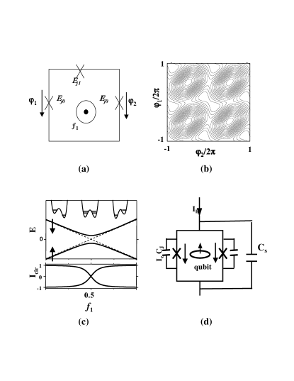
FIG. 1.: The superconducting flux qubit. (a) the circuit of the flux qubit. (b) the potential energy for the qubit. The black centers are local maxima and the white centers are local minima. (c) the energy and the average current of the qubit versus the flux. The arrows indicate the qubit states with opposite currents. The double well potentials at the corresponding flux are plotted. (d) the measurement of the qubit by a dc SQUID.

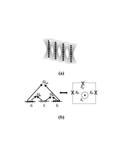
FIG. 2.: The atomic Josephson junction qubit. (a) Atoms trapped in the cigar-shaped optical potential by laser beams. (b) Left: the internal modes coupled by Raman pulses. Right: the superconducting flux qubit.

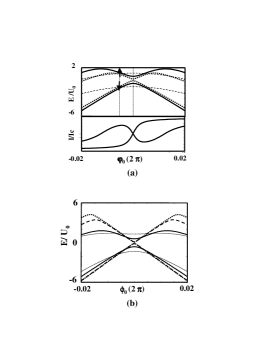
FIG. 3.: The energy and average current of the qubit states versus the phase $\phi_{0}$. (a) $N_{t}=15$ atoms. Solid lines: for symmetric interaction with $U_{0}=550\,{\rm Hz}$; dashed lines: for symmetric interaction with $U_{0}=0$; dotted lines: for interaction given in the text. (b) Energies of the qubit with various number of atoms for the symmetric interaction. Solid lines: $N_{t}=15$; thin dotted lines: $N_{t}=10$; dashed lines: $N_{t}=30$; dotted lines: $N_{t}=50$.

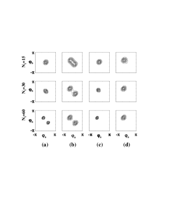
FIG. 4.: Contour plots of the probability $|\psi_{g}(\varphi_{a},\varphi_{b})|^{2}$ of the ground state wave function of the qubit: (a) $U_{0}=0.01$, $\phi_{0}=1/2$; (b) $U_{0}=0.2$, $\phi_{0}=1/2$; (c) $U_{0}=0.01$, $\phi_{0}=0.495$; (d) $U_{0}=0.2$, $\phi_{0}=0.495$.

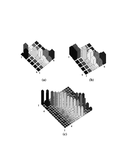
FIG. 5.: The absolute value of the elements of the unitary transformations for quantum logic gates, $|U_{ij}|$. The transformations are on the lowest six states of the qubits with the lowest two states the $|\uparrow\rangle$ and $|\downarrow\rangle$ states of the qubit. (a) single-qubit NOT gate. The labels indicate the lowest qubit states from $1$ to $6$. (b) single-qubit Hadamard gate. Labels are same as in (a). (c) two-qubit gate by a $36$-pulse sequence. The labels $1$ to $4$ are the qubit states: $|\uparrow\uparrow,\uparrow\downarrow,\downarrow\uparrow,\downarrow\downarrow\rangle$. The rest are higher states.

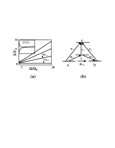
FIG. 6.: Adiabatic switching of Raman tunnelings. (a) The energy spectrum of the qubit versus the Raman coupling $\Omega$. The Raman coupling is plotted in unit of the Raman coupling $\Omega_{0}$ for the designed qubit. The energy differences between states $\Delta E_{12}$ and $\Delta E_{23}$ are indicated by arrows. The inset shows the average current $\langle I\rangle/\Omega$ in the same range of $\Omega$. (b) The laser pulse ${\cal H}_{m}$ of the QND measurement after the adiabatic switching. The coupling constants $\alpha_{2},\beta_{2},\gamma_{2}$ show the relative phase between the three components of the pulse.

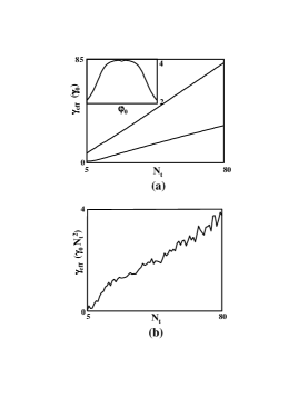
FIG. 7.: Decoherence rate by Eq. (18). (a) Single atom loss rate versus number of atoms. Inset: Single atom loss rate versus the phase $\phi_{0}$ of Raman coupling $\Omega_{ab}$. (b) Three-body loss rate in unit of $\gamma_{0}N_{t}^{2}$ versus the number of atoms.

REFERENCES

- [1] M. Tinkham, Introduction to Superconductivity, 2nd ed. (McGraw-Hill, New York, 1996).
- [2] T. P. Orlando and K. A. Delin, Introduction to Applied Superconductivity, (Addison and Wesley, Reading, MA, 1991).
- [3] A.J. Leggett, Rev. Mod. Phys. 73, 307 (2001).
- [4] D. S. Hall et al., Phys. Rev. Lett. 81, 1543 (1998); S. Inouye et al., Nature 392, 15 (1998); W. M. Liu, W. B. Fan, W. M. Zheng, J. Q. Liang, and S. T. Chui Phys. Rev. Lett. 88, 170408 (2002).
- [5] J. Javanainen, Phys. Rev. Lett. 57, 3164 (1986); I. Zapata, F. Sols, and A. J. Leggett, Phys. Rev. A 57, R28 (1998); J. Ruostekoski et al., Phys. Rev. A 57, 511 (1998); E. L. Bolda, S. M. Tan, and D. F. Walls, Phys. Rev. Lett. 79, 4719 (1997); R. Walser, Phys. Rev. Lett. 79, 4724 (1997); A. Smerzi, S. Fantoni, S. Giovanazzi, and S. R. Shenoy, Phys. Rev. Lett. 79, 4950 (1997); S. Giovanazzi, A. Smerzi, and S. Fantoni, Phys. Rev. Lett. 84 4521 (2000); S. Raghavan, A. Smerzi, S. Fantoni, and S. R. Shenoy, Phys. Rev. A 59, 620 (1999); J. R. Anglin, P. Drummond, and A. Smerzi, Phys. Rev. A64, 063605 (2001); J. R. Anglin and A. Vardi, Phys. Rev. A64, 013605 (2001).
- [6] Y. Makhlin, G. Schön, and A. Shnirman, Rev. Mod. Phys. 73, 357 (2001).
- [7] J.E. Mooij, T. P. Orlando, L. Levitov, Lin Tian, Caspar H. van der Wal, and Seth Lloyd, Science 285 , 1036 (1999).
- [8] T. P. Orlando, J. E. Mooij, Lin Tian, Caspar H. van der Wal, L. Levitov, Seth Lloyd, and J. J. Mazo, Phys. Rev. B 60, 15398 (1999).
- [9] K. Schulze, Diploma Thesis, University of Innsbruck (1999).
- [10] J.J. García-Ripoll and J. I. Cirac, Phys. Rev. Lett. 90, 127902 (2003); note that small fluctuation of the number of atoms does not affect our discussions on the qubit.
- [11] I. Chiorescu, Y. Nakamura, C. J. P. M. Harmans, and J. E. Mooij, Science 299, 1869 (2003).
- [12] D.P. DiVincenzo, Fortschritte der Physik special issue on Experimental Proposals for Quantum Computation, quant-ph/0002077.
- [13] Tin-Lun Ho, Phys. Rev. Lett.81, 742 (1998).
- [14] F.A. van Abeelen and B.J. Verhaar, Phys. Rev. A59, 578 (1999).
- [15] E. R. I. Abraham, W. I. McAlexander, J. M. Gerton, R. G. Hulet, R. Cote and A. Dalgarno, Phys. Rev. A55, R3299 (1997).
- [16] Let us introduce . Then the conjugates are . With and , the collision interaction is , which shows when compared with Eq. (12) in [8].
- [17] S. Lloyd, Phys. Rev. Lett.75, 346 (1995).
- [18] B. D. Esry, Chris H. Greene and James P. Burke, Jr., Phys. Rev. Lett. 83, 1751 (1999).
- [19] M.W. Jack, Phys. Rev. Lett.89, 140402 (2002).
- [20] A.J. Moerdijk, W.C. Stwalley, R.G. Hulet, and B.J. Verhaar, Phys. Rev. Lett. 72, 40 (1994); A.J. Moerdijk and B.J. Verhaar, Phys. Rev. Lett. 73, 518 (1994); A.J. Moerdijk, B.J. Verhaar, and A. Axelsson, Phys. Rev. A 51, 4852 (1995).