Entanglement Sharing in the Two-Atom Tavis-Cummings Model

Abstract

Individual members of an ensemble of identical systems coupled to a common probe can become entangled with one another, even when they do not interact directly. We investigate how this type of multipartite entanglement is generated in the context of a system consisting of two two-level atoms resonantly coupled to a single mode of the electromagnetic field. The dynamical evolution is studied in terms of the entanglements in the different bipartite partitions of the system, as quantified by the I-tangle. We also propose a generalization of the so-called residual tangle that quantifies the inherent three-body correlations in our tripartite system. This enables us to completely characterize the phenomenon of entanglement sharing in the case of the two-atom Tavis-Cummings model, a system of both theoretical and experimental interest.

I introduction

The control of quantum systems through active measurement and feedback has been developing at a rapid pace. In a typical scenario, a single atom is monitored indirectly through its coupling to a traveling probe such as a laser beam. The scattered beam and the system become correlated, and a subsequent measurement of the probe leads to backaction on the system. A coherent drive applied to the system can then be made conditional on the measurement record, leading to a closed-loop control model Wiseman (1994); Doherty et al. (2000). Such a protocol has been implemented to control a single mode electromagnetic field in a cavity Armen et al. (2002), and has been envisioned for controlling a variety of systems such as the state of a quantum dot in a solid Goan et al. (2001), the state of an atom coupled to a cavity mode Ye et al. (1999), and the motion of a micro-mechanical resonator coupled to a Cooper pair charge box Armour et al. (2002).

A common theme in the examples given above is that measurements are made on single copies of the quantum system of interest. However, in many situations one does not have access to an individually addressable system. In a gas, for example, preparing and/or addressing individual atoms is extremely difficult. In situations such as this, it is useful to think of the entire ensemble as a single many-body system. Indeed, recent experiments Kuzmich et al. (2000); Julsgaard et al. (2001) and theoretical proposals Thomsen et al. (2002) have explored the control of such ensembles from the point of view of the Dicke model Stockton et al. (2003), where a collection of $N$ two-level atoms is treated as a pseudo-spin with $J=N/2$.

Measurement backaction on the pseudo-spin can lead to squeezing of the quantum fluctuations Kuzmich et al. (2000); Julsgaard et al. (2001); Thomsen et al. (2002), which may be enhanced through active closed-loop control Wiseman (1994); Doherty et al. (2000). This squeezing can reduce the quantum fluctuations of an observable as in, for example, the reduction of “projection noise” leading to enhanced precision measurements in an atomic clock Wineland et al. (1994). Moreover, spin-squeezing is related to quantum entanglement between the atomic members of the ensemble Sorensen and Molmer (2001). This entanglement arises not through direct interaction between the atoms, but through their coupling to a common “quantum bus” in the form of an applied probe.

Measures of entanglement associated with these spin-squeezed states have been studied by Stockton, et. al., Stockton et al. (2003) under the assumption that all of the atoms in the ensemble are symmetrically coupled to the bus. However, completely quantifying entanglement in the most general cases is extremely difficult, and as yet, an unsolved problem Bruss (2002). In this article we consider the simplest possible ensemble consisting of two two-level atoms. Although at first sight this might appear trivial, when such a system is coupled to a quantum bus a rich structure emerges. Again, we consider the simplest realization of the bus – a single mode quantized electromagnetic field. The resulting physical system then corresponds to the two-atom Tavis-Cummings model (TCM) Tavis and Cummings (1968). A thorough understanding of the dynamical evolution of the TCM has obvious implications for the performance of quantum information processing Nielsen and Chuang (2000); Alber and et. al. (2001); Lo et al. (1998), as well as for our understanding of fundamental quantum mechanics Nielsen and Chuang (2000); Peres (1995). Bipartite entanglement has been investigated in this system for the one-atom case, known as the Jaynes-Cummings model, for initial pure states Loudon and Knight (1987) and mixed states Bose et al. (2001); Scheel et al. (2002) of the field.

Taken as a whole, the two-atom TCM in an overall pure state constitutes a tripartite quantum system in a Hilbert space with tensor product structure $2\otimes 2\otimes\infty$. Entanglement in tripartite systems has been studied by Coffman, et. al., Coffman et al. (2000) for the case of three qubits. They found that such quantum correlations cannot be arbitrarily distributed amongst the subsystems; the existence of three-body correlations constrains the distribution of the bipartite entanglement which remains after tracing over any one of the qubits. For example, in a GHZ-state, $|\mathrm{GHZ}\rangle=1/\sqrt{2}(|000\rangle+|111\rangle$), tracing over one qubit results in a maximally mixed state containing no entanglement between the remaining two qubits. In contrast, for a W-state, $|\mathrm{W}\rangle=1/\sqrt{3}(|001\rangle+|010\rangle+|100\rangle$), the average remaining bipartite entanglement is maximal Dur et al. (2000). Coffman, et. al., analyzed this phenomenon of entanglement sharing Coffman et al. (2000), using an entanglement monotone known as the tangle, a simple generalization of the more familiar concurrence Hill and Wootters (1997); Wootters (1998). They also introduced a new quantity known as the residual tangle, in order to quantify the irreducible tripartite correlations in a three qubit system Coffman et al. (2000).

In this article we extend the analysis of entanglement sharing to the case of the two-atom TCM. This has implications for the study of quantum control of ensembles. For example, if we imagine that the quantum bus is measured, e.g., the field leaks out of the cavity and is then detected, then the degree of correlation between the field and one of the atoms determines the degree of backaction on one atom. We can then quantify the degree to which one can perform quantum control on a single member of an ensemble even when one couples only collectively to the entire ensemble. We will accomplish this by extending the residual tangle formalism of Coffman, et. al., to our $2\otimes 2\otimes\infty$ system.

The remainder of this article is organized as follows. The important features of the TCM are reviewed in Sec. II, and the applicable measures of entanglement are introduced in Sec. III. With this formalism in hand, we calculate the tangle for each of the bipartite partitions of this tripartite system in Sec. IV. We will find an approximate analytic expression for the tangle between the field and the ensemble in the limit of large average photon number and in the Markoff approximation which provides further insight into these results. In Sec. V, we study the irreducible tripartite correlations in the system using our proposed generalization of the residual tangle. Finally, we summarize our results in section VI.

II The Tavis-Cummings Model

The Tavis-Cummings model (TCM) Tavis and Cummings (1968) (also known as the “Dicke model”Mandel and Wolf (1995)) describes the simplest fundamental interaction between a single mode of the quantized electromagnetic field and a collection of $N$ atoms under the usual two-level and rotating wave approximations. The two-atom $\left(N=2\right)$ TCM is governed by the Hamiltonian

$$H = H_{0}+H_{int}$$ (1)

$$= \hbar\omega\left(a^{\dagger}a+\frac{1}{2}\sigma_{z}^{\left(1\right)}+\frac{1}{2}\sigma_{z}^{\left(2\right)}\right)$$

$$+\hbar g\left[\left(\sigma_{-}^{\left(1\right)}+\sigma_{-}^{\left(2\right)}\right)a^{\dagger}+\left(\sigma_{+}^{\left(1\right)}+\sigma_{+}^{\left(2\right)}\right)a\right],$$

where $\sigma_{\pm}^{(i)}$ and $\sigma_{z}^{(i)}$ display a local $SU(2)$ algebra for the $i$-th atom in the two-dimensional subspace spanned by the ground and excited states $\{|g\rangle,|e\rangle\}$, and $a\left(a^{\dagger}\right)$ are bosonic annihilation (creation) operators for the monochromatic field. The Hilbert space ${\mathcal{H}}$ of the joint system is given by the tensor product ${\mathcal{H}}_{A_{1}}\otimes{\mathcal{H}}_{A_{2}}\otimes{\mathcal{H}}_{F}$ where ${\mathcal{H}}_{A_{1}}$ (${\mathcal{H}}_{A_{2}}$) denotes the Hilbert space of atom one (two) and ${\mathcal{H}}_{F}$ is the Hilbert space of the electromagnetic field.

The total number of excitations $K=a^{\dagger}a+\frac{1}{2}(\sigma_{z}^{(1)}+\sigma_{z}^{(2)}+2)$ is a conserved quantity which allows one to split the Hilbert space ${\mathcal{H}}$ into a direct sum of subspaces, i.e., ${\mathcal{H}}=\sum_{K=0}^{\infty}\oplus\Omega_{K}$, with each subspace $\Omega_{K}$ spanned by the eigenvectors $\{|ee,k-2\rangle,|eg,k-1\rangle,|ge,k-1\rangle,|gg,k\rangle\}$ of $K$ with eigenvalue $k$. The analytic form for the time evolution operator within a subspace $\Omega_{K}$ is given in Zeng, et. al., Zeng et al. (2001).

It is assumed throughout that the initial state of the TCM system is pure. Furthermore, we consider only the effects of the unitary evolution generated by Eq. (1), i.e., we do not include the effects of measurement, nor of mixing due to environment-induced decoherence Paz and Zurek (2002), so that our system remains in an overall pure state at all times. Finally, by assuming an identical coupling constant $g$ between each of the atoms and the field, the Hamiltonian is symmetric under atom-exchange. This invariance under the permutation group was used by Stockton, et. al., Stockton et al. (2003) to analyze the entanglement properties of very large ensembles. We will also make use of this fact in order to reduce the number of different partitioning schemes that one needs to consider when studying entanglement sharing in the two-atom TCM.

III The Tangle Formalism

The tangle between two qubits in an arbitrary state is defined in terms of the concurrence Hill and Wootters (1997); Wootters (1998). For a pure state $\left|\psi\right\rangle$ of two qubits, the concurrence is given by $C\left(\psi\right)\equiv\left|\left\langle\psi|\widetilde{\psi}\right\rangle\right|$, where $\left|\widetilde{\psi}\right\rangle$ represents the ‘spin-flip’ of $\left|\psi\right\rangle$, i.e., $\left|\widetilde{\psi}\right\rangle\equiv\sigma_{y}\otimes\sigma_{y}\left|\psi^{*}\right\rangle$, and the star denotes complex conjugation in the standard basis.

The generalization of the concurrence to a mixed state $\rho$ of two qubits is defined as the infimum of the average concurrence over all possible pure state ensemble decompositions of $\rho$, defined as convex combinations of pure states $S_{i}=\{p_{i},\psi_{i}\}$, such that $\rho=\sum_{i}p_{i}|\psi_{i}\rangle\langle\psi_{i}|$. In this way, $C\left(\rho\right)\equiv\inf_{S_{i}}\sum_{i}p_{i}C\left(\psi_{i}\right)=\inf_{S_{i}}\sum_{i}p_{i}\left|\left\langle\psi_{i}|\widetilde{\psi_{i}}\right\rangle\right|$. Wootters succeeded in deriving an analytic solution to this difficult minimization procedure in terms of the eigenvalues of the nonHermitian operator $\rho\widetilde{\rho}$, where the tilde again denotes the spin-flip of the quantum state. The closed form solution for the concurrence of a mixed state of two qubits is given by $C\left(\rho\right)=\max\left\{0,\lambda_{1}-\lambda_{2}-\lambda_{3}-\lambda_{4}\right\}$, where the $\lambda_{i}$’s are ordered in decreasing order Wootters (1998). Rungta, et. al., extended this formalism by introducing an analytic form for the concurrence of a bipartite system $AB$, with arbitrary dimensions $D_{A}$ and $D_{B}$, in an overall pure state Rungta et al. (2001). The analytic form of this quantity, dubbed the I-concurrence, is given by $C\left(\psi_{AB}\right)=\sqrt{2\nu_{A}\nu_{B}\left[1-tr\left(\rho_{A}^{2}\right)\right]}$, where $\rho_{A}$ is the marginal density operator obtained by tracing the joint pure state over subsystem $B$, and $\nu_{A}$ and $\nu_{B}$ are arbitrary scale factors.

Coffman, et. al., defined the tangle $\tau_{2}$ for a system of two qubits as the square of the concurrence Coffman et al. (2000), i.e.,

$$\tau_{2}\left(\rho\right)\equiv\max\left\{0,\lambda_{1}-\lambda_{2}-\lambda_{3}-\lambda_{4}\right\}^{2}.$$ (2)

Indeed, we may extend this definition directly to the result of Rungta, et. al., in order to obtain an analytic form for the tangle $\tau$ of a bipartite system in a pure state with arbitrary subsystem dimensions,

$$\tau\left(\psi_{AB}\right)\equiv C^{2}\left(\psi_{AB}\right)=2\nu_{A}\nu_{B}\left[1-tr\left(\rho_{A}^{2}\right)\right].$$ (3)

However, when extending this definition to apply to a bipartite mixed state $\rho_{AB}$ with arbitrary subsystem dimensions, one must find the infimum of the average squared pure state concurrence Osborne (2002)

$$\tau\left(\rho_{AB}\right) \equiv \inf_{S_{i}}\sum_{i}p_{i}C^{2}\left(\psi_{AB}^{\left(i\right)}\right)$$ (4)

$$= 2\nu_{A}\nu_{B}\inf_{S_{i}}\sum_{i}p_{i}\left\{1-tr\left[\left(\rho_{A}^{\left(i\right)}\right)^{2}\right]\right\},$$

where we have used Eq. (3) for the pure state tangle with $\rho_{A}^{(i)}$ as the marginal state for the $i^{\mathrm{th}}$ term in the ensemble decomposition.

At this point we note that the scale factors $\nu_{A}$ and $\nu_{B}$ in Eqs. (3) and (4), which may in general depend on the dimensions of the subsystems $D_{A}$ and $D_{B}$ respectively, are usually set to one so that agreement with the two qubit case is maintained, and so that the addition of extra unused Hilbert space dimensions has no effect on the value of the concurrence Rungta et al. (2001). We will find in Sect. V, when we attempt our own further generalization of the tangle formalism, that it is useful to take advantage of this scale freedom. For now, however, we adopt the usual convention both for the sake of clarity, and to demonstrate exactly where in our proposed generalization this freedom is required.

Using the definition given by Eq. (4), dubbed the I-tangle in reference to the work of Rungta, et. al., Osborne derived an analytic form for $\tau\left(\rho_{AB}\right)$ in the case where the rank of $\rho_{AB}$ is no greater than two,

$$\tau\left(\rho_{AB}\right)=tr\left(\rho_{AB}\widetilde{\rho}_{AB}\right)+2\lambda_{min}^{\left(AB\right)}\left[1-tr\left(\rho_{AB}^{2}\right)\right],$$ (5)

where $\widetilde{\rho}_{AB}$ now represents the universal inversion Rungta et al. (2001) of $\rho_{AB}$, and $\lambda_{min}^{\left(AB\right)}$ is the smallest eigenvalue of the $M$ matrix defined by Osborne Osborne (2002). The important point is that Eq. (5) yields a closed form which, as we will see in Sect. IV.3, is directly applicable to a specific bipartite partition of the two-atom TCM.

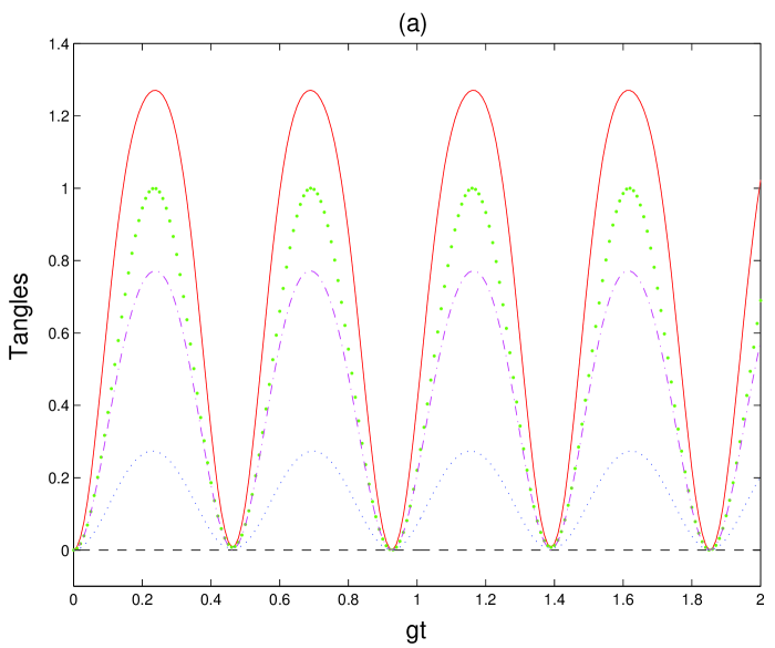
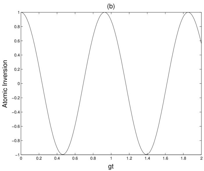
Figure 1: (Color online) TCM evolution for both atoms initially in the excited state and the field in an initial Fock state with $n=10$. (a) Solid curve (red): Field-ensemble tangle $\tau_{F\left(A_{1}A_{2}\right)}$; Large-dotted curve (green): One atom-remainder tangle $\tau_{A_{1}\left(A_{2}F\right)}$; Dashed curve (black): Atom-atom tangle $\tau_{A_{1}A_{2}}$(Note that the atom-atom tangle is always zero for the given initial condition); Dot-dashed curve (pink): Single atom-field tangle $\tau_{A_{1}F}$; Dotted curve (blue): Residual tangle $\tau_{A_{1}A_{2}F}$. (b) Atomic inversion of the ensemble.

IV Bipartite Tangles in the Two-Atom TCM

Let the two atoms in the ensemble be denoted by $A_{1}$ and $A_{2}$, respectively, and the field, or quantum bus, by $F$. Because of the assumed exchange symmetry, there are four nonequivalent partitions of the two-atom TCM into tensor products of bipartite subsystems: (i) the field times the two-atom ensemble, $F\otimes(A_{1}A_{2})$, (ii) one atom times the remaining atom and the field, $A_{1}\otimes(A_{2}F)\equiv A_{2}\otimes(A_{1}F)$, (iii) the two atoms taken separately, having traced over the field, $A_{1}\otimes A_{2}$, and (iv) one of the atoms times the field, having traced over the other atom, $A_{1}\otimes F\equiv A_{2}\otimes F$. We calculate how the tangle for each of these partitions evolves as a function of time under TCM Hamiltonian evolution using the formalism reviewed in Sec. II. We take the initial state to be a pure product state of the field with the atoms. We will capture the key features of the tangle evolution by considering three classes of initial state vectors,

$$\left|e\right\rangle_{A_{1}}\otimes\left|e\right\rangle_{A_{2}}\otimes\left|n\right\rangle_{F}\equiv\left|ee,n\right\rangle,$$ (6a)

$$\left|ee,\alpha\right\rangle or\left|gg,\alpha\right\rangle,$$ (6b)

and

$$\frac{1}{\sqrt{2}}\left(\left|eg\right\rangle+\left|ge\right\rangle\right)\otimes\left|\alpha\right\rangle or\,\frac{1}{\sqrt{2}}\left(\left|gg\right\rangle+\left|ee\right\rangle\right)\otimes\left|\alpha\right\rangle,$$ (6c)

where $\left|g(e)\right\rangle$ denotes the ground (excited) state of the atom, $\left|n\right\rangle$ denotes a Fock state field with $n$ photons, and $\left|\alpha\right\rangle$ denotes a coherent state field with an average number of photons given by $\left\langle n\right\rangle$. The alternatives in Eqs. (6b) and (6c) arise from the fact that, in the limit of large $\left\langle n\right\rangle$, the evolution of all of the tangles are found to be identical for the two different initial atomic conditions, as we will see below.

IV.1 Field-Ensemble and One Atom-Remainder Tangles

Under the assumption that the system is in an overall pure state, we may easily calculate the tangles in partitions (i) and (ii) above by applying Eq. (3), with $\nu_{A}=\nu_{B}=1$. Specifically,

$$\tau_{F\left(A_{1}A_{2}\right)}=2\left[1-tr\left(\rho_{F}^{2}\right)\right]=2\left[1-tr\left(\rho_{A_{1}A_{2}}^{2}\right)\right],$$ (7)

and

$$\tau_{A_{1}\left(A_{2}F\right)}=2\left[1-tr\left(\rho_{A_{1}}^{2}\right)\right]=2\left[1-tr\left(\rho_{A_{2}F}^{2}\right)\right],$$ (8)

where we have used the fact that the (nonzero) eigenvalue spectra of the two marginal density operators for a bipartite division of a pure state are identical Nielsen and Chuang (2000); Ekert and Knight (1995) in obtaining the rightmost equalities. These tangles have implications for the quantum control of atomic ensembles. Because the overall system is pure, any correlation between the field and the ensemble is necessarily in one-to-one correspondence with the amount of entanglement between these two subsystems. The quantum backaction on the ensemble due to measurement of the field is thus quantified by Eq. (7). Alternatively, a measurement of one atom leads to backaction on the remaining subsystem as described by Eq. (8).

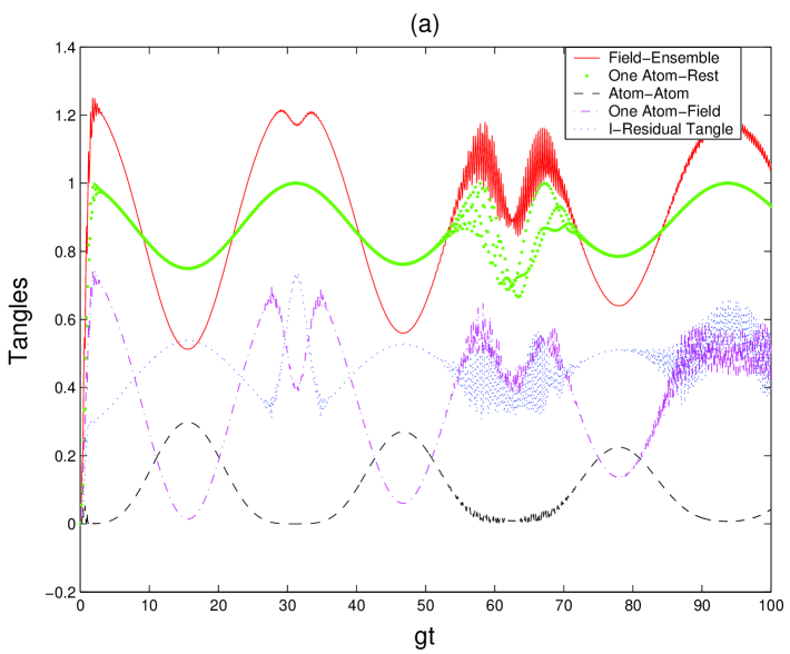
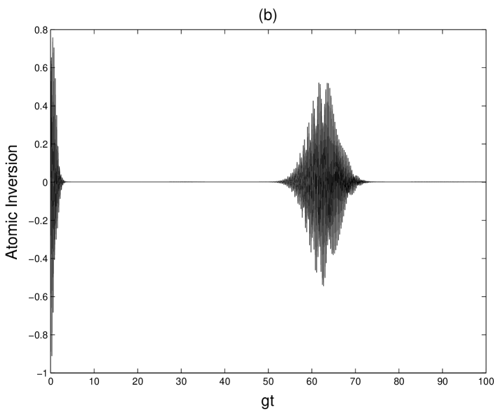
Figure 2: (Color online) TCM evolution for both atoms initially in a stretched state and the field in an initial coherent state with $\left\langle n\right\rangle=100.$ (a) Solid curve (red): Field-ensemble tangle $\tau_{F\left(A_{1}A_{2}\right)}$; Large-dotted curve (green): One atom-remainder tangle $\tau_{A_{1}\left(A_{2}F\right)}$; Dashed curve (black): Atom-atom tangle $\tau_{A_{1}A_{2}}$; Dot-dashed curve (pink): Single atom-field tangle $\tau_{A_{1}F}$; Dotted curve (blue): Residual tangle $\tau_{A_{1}A_{2}F}$. (b) Atomic inversion of the ensemble.

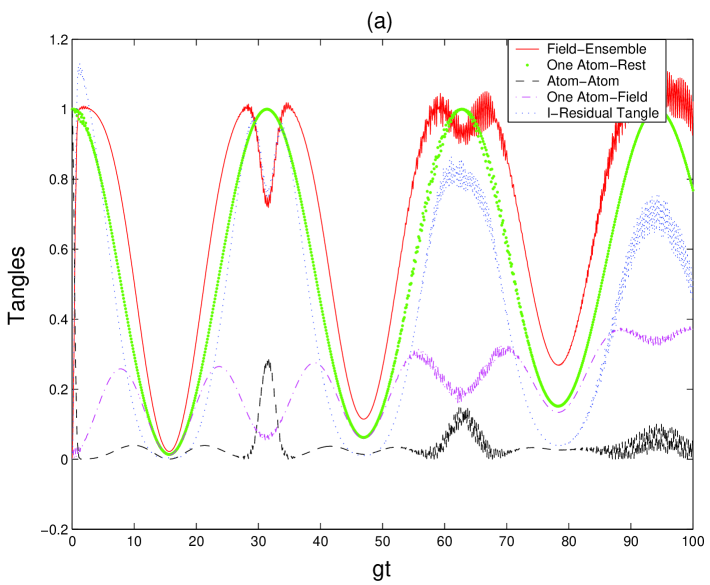
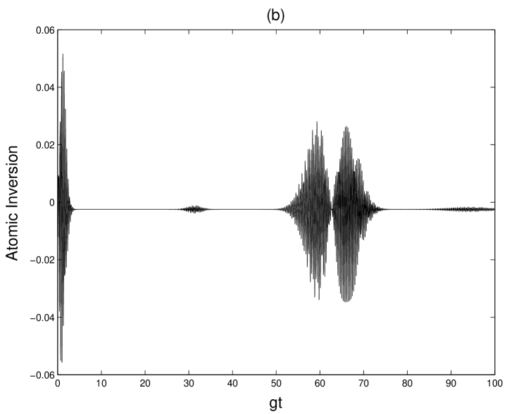
Figure 3: (Color online) TCM evolution for the atoms initially in one of the symmetric states and the field in an initial coherent state with $\left\langle n\right\rangle=100.$ (a) Solid curve (red): Field-ensemble tangle $\tau_{F\left(A_{1}A_{2}\right)}$; Large-dotted curve (green): One atom-remainder tangle $\tau_{A_{1}\left(A_{2}F\right)}$; Dashed curve (black): Atom-atom tangle $\tau_{A_{1}A_{2}}$; Dot-dashed curve (pink): Single atom-field tangle $\tau_{A_{1}F}$; Dotted curve (blue): Residual tangle $\tau_{A_{1}A_{2}F}$. (b) Atomic inversion of the ensemble.

The time evolutions for each of the different tangles, corresponding to the initial conditions given by Eqs. (6a) - (6c), are shown in Figs. 1(a) - 3(a) respectively. Figs. 1(b) - 3(b) show the time evolution of the atomic inversion, defined as the probability of finding both atoms in the excited state minus the probability of finding both atoms in the ground state, for reference purposes. We find, under certain conditions, that the two stretched states in Eq. (6b) lead to identical evolution for the tangles in all of the bipartite partitions of the system, corresponding to the curves shown in Fig. 2(a). Similarly, the two symmetric states given in Eq. (6c) both yield the curves shown in Fig. 3(a). This behavior can be derived under a set of highly accurate approximations. In the limit of large average photon number, an initial coherent state field with zero phase will remain approximately separable from the atomic ensemble in an eigenstate of $J_{x}\equiv J_{+}+J_{-}$ up to times on the order of $\left\langle n\right\rangle/{g}$ where, in the pseudospin picture, $J_{\pm}\equiv\sigma^{(1)}_{\pm}+\sigma^{(2)}_{\pm}$. This follows immediately from the time evolution operator generated by $H_{int}$ in Eq. (1) in the interaction picture. The key observation is that, for a macroscopic field, the removal or addition of a single photon has a negligible effect. This allows one to approximate the time evolution operator by $\exp^{-iH_{int}t/\hbar}\approx\exp^{-ig\sqrt{\left\langle n\right\rangle}J_{x}t}$. Thus, the eigenstates of $J_{x}$ form a convenient basis to use in describing the state of the atomic ensemble. This approach was taken by Gea-Banacloche in analyzing the behavior of the single atom Jaynes-Cummings model Gea-Banacloche (1990) and the generation of macroscopic superposition states Gea-Banacloche (1991), and extended to the multi-atom TCM by Chumakov, et. al., Chumakov et al. (1994); Delgado et al. (1998); Saavedra et al. (1998).

We take as the appropriate basis the three symmetric eigenstates of $J_{x}$, which we label by $m=$ -1, 0, and 1; the singlet state, $J=0$, is a dark state and thus does not couple to the field. Writing the initial state of the system as

$$\left|\psi(0)\right\rangle=\sum_{m=-1}^{1}d_{m}\left|m\right\rangle\otimes\left|\alpha\right\rangle,$$ (9)

and using the factorization approximation Chumakov et al. (1994), we find that the state of the system up to times on the order of $\left\langle n\right\rangle/{g}$ is given by

$$\left|\psi(t)\right\rangle\approx\sum_{m=-1}^{1}d_{m}\left|A_{m}(t)\right\rangle\otimes\left|\phi_{m}(t)\right\rangle,$$ (10)

where $\left|A_{m}(t)\right\rangle$ and $\left|\phi_{m}(t)\right\rangle$ are the time-evolved atomic and field states, respectively. The marginal density operator for the two atoms is then

$$\rho_{A_{1}A_{2}}(t)\approx\sum_{l,m}d_{l}^{*}d_{m}\left|A_{m}(t)\right\rangle\left\langle A_{l}(t)\right|f_{ml}\left(gt,\left\langle n\right\rangle\right),$$ (11)

where $f_{ml}\left(gt,\left\langle n\right\rangle\right)\equiv\sum_{n}\left\langle n\mid\phi_{m}(t)\right\rangle\left\langle\phi_{l}(t)\mid n\right\rangle$. We find that this function has “memory” only for $t\ll\sqrt{\left\langle n\right\rangle}/{g}$, and behaves very much like a delta function for longer time scales. Effectively, the large dimensional Hilbert space of the field acts as a broadband reservoir for the atoms – the generalization of the familiar “collapse” phenomenon in the Jaynes-Cummings model. This “Markoff” approximation is valid up to times on the order of $2\pi\sqrt{\left\langle n\right\rangle}/{g}$, corresponding to the well-known revival time in the Jaynes-Cummings Model Gea-Banacloche (1990). Making this approximation in Eq. (11), the states $\left|A_{m}\left(t\right)\right\rangle$ act effectively as a “pointer basis” for decoherence Paz and Zurek (2002) of the atomic density matrix, i.e.,

$$\rho_{A_{1}A_{2}}(t)\approx\sum_{m}\left|d_{m}\right|^{2}\left|A_{m}(t)\right\rangle\left\langle A_{m}(t)\right|.$$ (12)

Substituting this formula into Eq. (7) yields

$$\tau_{F\left(A_{1}A_{2}\right)}(t)\approx 2\left\{1-\frac{1}{4}\left[c-h(t^{\prime})\right]\right\},$$ (13)

where

$$c \equiv 4\left(\left|d_{-1}\right|^{4}+\left|d_{0}\right|^{4}+\left|d_{1}\right|^{4}\right)+2\left|d_{0}\right|^{2}\left|d_{1}\right|^{2}$$ (14)

$$+\left|d_{-1}\right|^{2}\left(2\left|d_{0}\right|^{2}+3\left|d_{1}\right|^{2}\right)-4\left|d_{-1}\right|^{2}\left|d_{1}\right|^{2}$$

$$h\left(t^{\prime}\right) \equiv 2\left|d_{0}\right|^{2}\left(\left|d_{-1}\right|^{2}+\left|d_{1}\right|^{2}\right)\cos\left(4t^{\prime}\right)$$ (15)

$$+\left|d_{-1}\right|^{2}\left|d_{1}\right|^{2}\cos\left(8t^{\prime}\right),$$

and

$$t^{\prime}\equiv\frac{gt}{2\sqrt{\left\langle n\right\rangle-\frac{N}{2}+\frac{1}{2}}}.$$ (16)

Under the factorization and Markoff approximations, the field-ensemble tangle is given by a constant term $c$ that depends only on the initial probabilities to find the atomic ensemble in each of the $J_{x}$ eigenstates, and a time-dependent piece $h(t^{\prime})$. These probabilities depend solely on the absolute squares of the expansion coefficients of the initial atomic state given by Eq. (9). It is now clear why certain initial atomic conditions result in identical evolution for the different tangles. For example, the initial atomic states $\left|gg\right\rangle$ and $\left|ee\right\rangle$ both satisfy

$$\left|d_{-1}\right|=\left|d_{1}\right|=\frac{1}{2}\,and\,\left|d_{0}\right|=\frac{1}{\sqrt{2}},$$ (17)

corresponding to identical evolution for all of the tangles shown in Fig. 2(a). Similarly, the initial atomic states ${1}/\sqrt{2}\left(\left|eg\right\rangle+\left|ge\right\rangle\right)$ and ${1}/\sqrt{2}\left(\left|ee\right\rangle+\left|gg\right\rangle\right)$ both satisfy

$$\left|d_{-1}\right|=\left|d_{1}\right|=\frac{1}{\sqrt{2}}\,and\,\left|d_{0}\right|=0,$$ (18)

corresponding to the curves shown in Fig. 3(a). More generally, this property holds for any class of initial states $\left|\psi^{(i)}\left(0\right)\right\rangle$ having the form of Eq. (9) such that $\left|d_{m}^{(i)}\right|=\left|d^{(j)}_{m}\right|$, $m\in\left\{-1,0,1\right\}$. One immediate consequence of this result is that the relative phase information encoded in the initial state of the atomic system is irrelevant to the evolution of the field-ensemble tangle.

The field-ensemble tangle calculated according to Eq. (7) and the approximation given by Eq. (13) for an initial stretched atomic state and an initial coherent state field with $\left\langle n\right\rangle=500$ are shown by the solid (red) and dashed (black) curves in Fig. 4, respectively. The approximation is seen to track the exact evolution extremely well over the range of its validity. The discrepancy at very small times is explained by the fact that at these times the Markoff approximation breaks down. It is also seen that our approximate solution does not capture the small dip in the field-ensemble tangle occurring at $t=\pi\sqrt{\left\langle n\right\rangle}/{g}$. The absence of this feature can be explained by noting that in making the Markoff approximation we have effectively wiped out any information regarding the initial coherence between the $\left|m=-1\right\rangle$ and $\left|m=1\right\rangle$ states. The presence of this dip is then seen to be dependent upon the existence of this coherence. This is borne out by the fact that the dip in the field-ensemble tangle in Fig. 2(a) is much shallower than that in Fig. 3(a), where the initial atomic expansion coefficients are given by Eqs. (17) and (18), respectively.

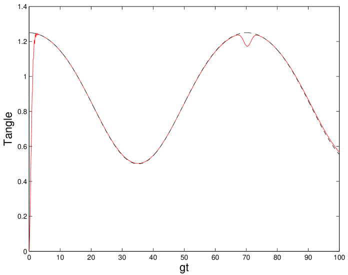
Figure 4: (Color online) Exact field-ensemble tangle: Solid (red) curve, and approximate formula: Dashed (black) curve, as functions of time.

IV.2 Atom-Atom Tangle

Given an initial state, we time-evolve the system according to the dynamics governed by Eq. (1), and then trace over the field subsystem. The tangle of the two-atom mixed state $\rho_{A_{1}A_{2}}\left(t\right)$ may then be calculated according to Eq. (2). The resulting atom-atom tangles corresponding to the initial conditions in Eqs. (6a) - (6c) are depicted by the dashed (black) curves in Figs. 1(a) - 3(a), respectively. These curves yield direct insight into the state of the atomic ensemble as a function of time. Specifically, the atom-atom tangle quantifies the degree to which the ensemble behaves as a collective entity, rather than as two individual particles.

It is somewhat surprising that for the initial condition given by Eq. (6a), i.e., when the field is initially in a Fock state with any value for $n$, the atom-atom tangle remains zero at all times, whereas the evolution of the atom-atom tangle resulting from an initial coherent state field is nontrivial and, in general, nonzero. As a first step towards understanding these observations, we have studied the evolution of the atom-atom tangle for other initial conditions. When the field is initially in a Fock state and both atoms start in the ground state, the loss of an excitation in the field can result in the creation of an excitation in the atomic ensemble. This produces entanglement between the field and the ensemble and in the single atom-field and one atom-remainder partitions. Since it is not possible to distinguish in which atom the excitation is created, the two atoms become entangled with each other as well. It is found that the atom-atom entanglement falls off as $1/{n}^{2}$ so that, in the limit of a highly excited Fock state, these initial conditions yield results reminiscent of those found in Fig. 1(a). Specifically, we find that the entanglement in all of the different subsystem partitions always oscillate in phase at twice the Rabi frequency, and that the atom-atom tangle approaches zero as ${n}$ becomes large.

Next, we considered the case when both atoms initially reside in a stretched state, and the initial field state consists of a coherent superposition of two neighboring Fock states. We find, on a time scale much longer than that given by the inverse of the associated Rabi frequencies, that the overall behavior again closely resembles the evolution seen for an initial field consisting of a single Fock state. Specifically, we find that the general features of all of the different bipartite tangles oscillate in phase with one another. However, on much shorter time-scales, the effects of dephasing between the two Rabi frequencies become apparent, yielding the first clues regarding how the observed coherent state behavior arises in terms of initial Fock state superpositions. For example, it seems likely that these observations provide insight into the Fock-like behavior seen in Fig. 2(a) at the revival time, when there is a partial rephasing of the Rabi frequencies. At this time all of the bipartite tangles decrease simultaneously, while at other times the tangles in certain bipartite partitions may be completely out of phase with one another. We are currently performing a detailed study of the entanglement that can be dynamically generated between the two atoms under TCM evolution for the most general initial conditions in order to better understand this behavior.

IV.3 Single Atom-Field Tangle

The final bipartite partition of the two-atom TCM is that consisting of a single atom, say $A_{1}$, as one subsystem and the field $F$ as the second subsystem. Again by exchange symmetry $\tau_{A_{1}F}=\tau_{A_{2}F}$, so we need calculate only one of these quantities. Because the tripartite system is in an overall pure state, the Schmidt decomposition theorem Nielsen and Chuang (2000); Ekert and Knight (1995) implies that the marginal density operator $\rho_{A_{1}F}$ has at most rank two. The rank of the reduced density matrix is set by the dimension of the smallest subsystem, which in this case is a two-level atom. This is exactly the scenario envisioned by Osborne Osborne (2002), as described in Sec. III. The tangle corresponding to this partition, $A_{1}\otimes F$, is computed by first tracing over the state of the remaining atom, $A_{2}$, and then applying Eq. (5).

Employing this procedure,

$$\tau_{A_{1}F}=tr\left(\rho_{A_{1}F}\widetilde{\rho}_{A_{1}F}\right)+2\lambda^{\left(A_{1}F\right)}_{min}\left[1-tr\left(\rho_{A_{1}F}^{2}\right)\right],$$ (19)

where $\lambda_{min}^{\left(A_{1}F\right)}$ represents the minimum eigenvalue of the Osborne $M$ matrix Osborne (2002) generated from the marginal density operator $\rho_{A_{1}F}$. The dot-dashed (pink) curves in Figs. 1(a) - 3(a) give the time evolution of the single atom-field tangle for the different initial conditions considered.

We are now in possession of closed forms for the tangles of all bipartite partitions of the two-atom TCM. Any other entanglement that the system may possess must necessarily be in the form of irreducible three-body quantum correlations. In section V we review the residual tangle formalism introduced by Coffman, et. al., in order to quantify this type of tripartite entanglement in a system of three qubits. We then propose a generalization of this quantity that is applicable to a $2\otimes 2\otimes D$ system in an overall pure state. This extension of the tangle formalism allows us to study the phenomenon of entanglement sharing in the two-atom TCM.

V Entanglement Sharing and the Residual Tangle

The concept of entanglement sharing studied in Coffman et al. (2000); Dennison and Wootters (2001) refers to the fact that entanglement cannot be freely distributed among subsystems in a multipartite, i.e., tripartite or higher, system. Rather, the distribution of entanglement in these systems is subject to certain constraints. As a simple example, consider a tripartite system of three qubits labeled $A,$ $B,$ and $C.$ Suppose that qubits $A$ and $B$ are known to be in a maximally entangled pure state, e.g., the singlet state, given by $\left|\psi_{AB}\right\rangle=1/\sqrt{2}\left(\left|01\right\rangle-\left|10\right\rangle\right)$ when written in the logical basis. In this case, it is obvious that the overall system $ABC$ is constrained such that no entanglement may exist either between $A$ and $C$ or between $B$ and $C.$ Otherwise, tracing over subsystem $C$ would necessarily result in a mixed marginal density operator for $AB$ in contradiction to the known purity of the singlet state.

Coffman, et. al., analyze the phenomenon of entanglement sharing for a system of three qubits in an overall pure state in full generality by introducing a quantity known as the residual tangle Coffman et al. (2000). This definition is motivated by the observation that the tangle of $A$ with $B$ plus the tangle of $A$ with $C$ cannot exceed the tangle of $A$ with the joint subsystem $BC$, i.e.,

$$\tau_{AB}+\tau_{AC}\leq\tau_{A\left(BC\right)}.$$ (20)

Here, $\tau_{AB}$ and $\tau_{AC}$ are calculated according to Eq. (2), and $\tau_{A\left(BC\right)}$ may be obtained from Eq. (3).

The original proof Coffman et al. (2000) of the inequality in Eq. (20), which forms the heart of the phenomenon of entanglement sharing for the case of three qubits, may be substantially simplified by making use of certain results due to Rungta, et. al. Specifically, we note that Rungta et al. (2001)

$$tr\left(\rho_{xy}\widetilde{\rho}_{xy}\right)=1-tr\left(\rho_{x}^{2}\right)-tr\left(\rho_{y}^{2}\right)+tr\left(\rho_{xy}^{2}\right)\geq 0$$ (21)

for subsystems $x$ and $y$ having arbitrary Hilbert space dimensions. Under the assumption that $x$ and $y$ are in an overall pure state with a third subsystem $z$, Eq. (21) may be rewritten

$$tr\left(\rho_{xy}\widetilde{\rho}_{xy}\right)=1-tr\left(\rho_{x}^{2}\right)-tr\left(\rho_{y}^{2}\right)+tr\left(\rho_{z}^{2}\right)\geq 0,$$ (22)

where we have used the equality of the nonzero eigenvalue spectra of $\rho_{xy}$ and $\rho_{z}$. Then, by the observation Coffman et al. (2000) that for an arbitrary state of two qubits $A$ and $B,$ the following upper bound on the tangle defined by Eq. (2) holds

$$\tau_{2}\left(\rho_{AB}\right)\leq tr\left(\rho_{AB}\widetilde{\rho}_{AB}\right),$$ (23)

and by Eq. (3) with $\nu_{A}=\nu_{B}=1$, the inequality in Eq. (20) follows immediately.

Subtracting the terms on the left hand side of Eq. (20) from that on the right hand side yields a positive quantity referred to as the residual tangle $\tau_{ABC}$, i.e.,

$$\tau_{ABC}\equiv\tau_{A\left(BC\right)}-\tau_{AB}-\tau_{AC}.$$ (24)

The residual tangle is interpreted as quantifying the inherent tripartite entanglement present in a system of three qubits, i.e., the entanglement that cannot be accounted for in terms of the various bipartite tangles. This interpretation is given further support by the observation that the residual tangle is invariant under all possible permutations of the subsystem labels Coffman et al. (2000).

We wish to generalize the residual tangle, defined for a system of three qubits, to apply to a $2\otimes 2\otimes D$ quantum system in an overall pure state so that we may study entanglement sharing in the two-atom TCM. Note that we already have all of the other tools needed for such an analysis. Specifically, from section IV, we know the analytic forms for all of the different possible bipartite tangles in such a system.

Any proper generalization of the residual tangle must, at a minimum, be a positive quantity, and be equal to zero if and only if there is no tripartite entanglement in the system, i.e., if and only if all of the quantum correlations can be accounted for using only bipartite tangles. It should also reduce to the definition of the residual tangle in the case of three qubits. Further it is reasonable to require, if this is to be a true measure of irreducible three-body correlations, that symmetry under permutation of the subsystems be preserved, and that it remain invariant under local unitary operations. Finally, we conjecture that this quantity satisfies the requirements for being an entanglement monotone Vedral et al. (1997); Vidal (2000) under the set of stochastic local operations and classical communication (SLOCCs), or equivalently, under the set of invertible local operations Dur et al. (2000). We limit the monotonicity requirement to this restricted set of operations since, in the context of entanglement sharing, we are only concerned with LOCCs that preserve the local ranks of the marginal density operators such that all subsystem dimensions remain constant.

Let $A$ and $B$ again be qubits, and let $C$ now be a $D$-dimensional system with the composite system $ABC$ in an overall pure state. We note that, under these assumptions, we are still capable of evaluating each of the terms on the right hand side of Eq. (24) analytically using the results of section IV. However, we cannot simply use the definition of the residual tangle (with $C$ now understood to represent a $D$-dimensional system) as the proper generalization for two reasons. First, since the three subsystems are no longer of equal dimension, symmetry under permutations of the subsystems is lost. However, as we will see, this problem is easily fixed by explicitly enforcing the desired symmetry. The second, and more difficult problem to overcome is the fact that the inequality given by Eq. (20) no longer holds for our generalized system because $\lambda_{min}$ in Eq. (5) can be negative, implying that Eq. (24) can also be negative.

The required permutation symmetry may be restored by taking our generalization of the residual tangle, which we dub the I-residual tangle in reference to previous work and continue to denote by $\tau_{ABC}$, to be

$$\tau_{ABC} \equiv \frac{1}{3}\left(\tau_{A\left(BC\right)}+\tau_{B\left(AC\right)}+\tau_{C\left(AB\right)}\right)$$ (25)

$$-\frac{2}{3}\left(\tau_{AB}+\tau_{AC}+\tau_{BC}\right)$$

The definition in Eq. (25) is obtained by averaging over all possible relabelings of the subsystems in Eq. (24). By inspection, it is obvious that Eq. (25) preserves permutation symmetry. However, it still suffers from the problem that its value can be negative. In order to deal with this difficulty, we make use of the arbitrary scale factors appearing in Eqs. (3) and (4), and discussed in section III.

Let $d$ be the smaller of the two ‘dimensions’ of two arbitrary dimensional subsystems $x$ and $y$, i.e., $d\equiv\min\left\{D_{x},D_{y}\right\}$. Note that by dimension we do not necessarily mean the total Hilbert space dimension of the physical system under consideration, but only the number of different Hilbert space dimensions that contribute to the formation of the overall pure state of the system. This is a subtle but important point which automatically enforces insights like those due to Rungta, et. al., Rungta et al. (2001) and Verstraete, et. al., Verstraete et al. (2001) which state that the scale chosen for a measure of entanglement must be invariant under the addition of extra, but unused, Hilbert space dimensions. The two-atom TCM provides one example of the relevant physics underlying these ideas.

Consider, for example, the bipartite partitioning of the TCM into a field subsystem with $D_{F}=\infty$, and an ensemble subsystem consisting of the two qubits with $D_{A_{1}A_{2}}=4$. Any entangled state of the overall system has a Schmidt decomposition with at most four terms, implying that the field effectively behaves like a four-dimensional system. Further, since the Tavis-Cummings Hamiltonian given by Eq. (1) does not induce couplings between the field and the singlet state of the atomic ensemble, i.e., the singlet state is a dark state, the field behaves effectively as a three-level system, or qutrit, in the context of the TCM. Accordingly, in any entangled state of the field with the ensemble, the field is considered to have a dimension no greater than three. We employ this revised definition of dimension throughout the remainder of the paper.

We now make the choice

$$\nu_{A}\nu_{B}={d}/{2},$$ (26)

when calculating each of the bipartite tangles appearing on the right hand side of Eq. (25). This choice is made for several reasons. First of all, it is in complete agreement with the two qubit case, yielding $\nu_{A}\nu_{B}=1$ as required. Indeed, when $A$, $B$, and $C$ are all qubits, the residual tangle given by Eq. (24) is recovered. Secondly, it takes differences in the Hilbert space dimensions of the subsystems into account when setting the relevant scale for each tangle. This is important since, in order to study the phenomenon of entanglement sharing, the tangles for each of the different bipartite partitions must be compared on a common scale. It is reasonable that this scale be a function of the smaller of the two subsystem dimensions since, for an overall pure state, it is this quantity that limits the number of terms in the Schmidt decomposition. Finally, it is conjectured that a proper rescaling of the various tangles will result in the positivity of Eq. (25).

Note that when applying the proposed rescaling to the terms on the right hand side of Eq. (25), the only term affected is $\tau_{C\left(AB\right)}$, which is rescaled by one-half of the smaller of the two subsystem dimensions $D_{C}$ and $D_{AB}$. Each of the other terms remains unaltered since, in each case, at least one of the two subsystems involved is a qubit. The net effect of this rescaling is to increase the ‘weight’ of the tangle between $C$ and $AB$ relative to that of the rest of the tangles. This is reasonable when one recognizes that both $AB$, a system of two qubits, and $C$, a $D$-dimensional system (in the case $D>2$), have entanglement capacities Dennison and Wootters (2001) exceeding that of a single qubit.

The requirement that the I-residual tangle be invariant under local unitary operations follows trivially, since each term on the right hand side of Eq. (25) is known to satisfy this property individually. It is still an open question as to whether or not the proposed rescaling is sufficient to preserve positivity when generalizing the residual tangle, Eq. (24), to the I-residual tangle, Eq. (25). However, numerical calculations give strong evidence that this is the case. The I-residual tangle has been calculated for over two-hundred million randomly generated pure states of a $2\otimes 2\otimes 3$ system and of a $2\otimes 2\otimes 4$ system, the only nontrivial possibilities. In each instance the resulting quantity has been positive. We conjecture that the I-residual tangle satisfies the requirements of positivity and monotonicity under SLOCC not only for a $2\otimes 2\otimes D$ system, where closed forms currently exist for all of the terms on the right hand side of Eq. (25), but for the most general ${D}_{A}\otimes{D}_{B}\otimes{D}_{C}$ dimensional tripartite system in an overall pure state (with the proper scaling of each term again given by Eq. (26)). The I-residual tangle arising in the context of the two-atom TCM is shown by the blue curves in Figs. 1(a) - 3(a).

The residual tangle, as well as our proposed generalization of this quantity, may be interpreted as the irreducible tripartite entanglement in a system since it cannot be accounted for in terms of any combination of bipartite entanglement measures Coffman et al. (2000). A slightly different, and possibly more enlightening interpretation is that the I-residual tangle quantifies the amount of ‘freedom’ that a system has in satisfying the constraints imposed by the phenomenon of entanglement sharing. If the I-residual tangle of a tripartite system is zero, then each bipartite tangle is uniquely determined by the values of all of the other bipartite tangles. Alternatively, if $\tau_{ABC}$ is strictly greater than zero, then the bipartite tangles enjoy a certain latitude in the values that each may assume while still satisfying the positivity criterion. The larger the value of the I-residual tangle, the more freedom the system has in satisfying the entanglement sharing constraints. This reasoning highlights the relationship between entanglement sharing and the I-residual tangle.

Finally, we may interpret the I-residual tangle as the average fragility of a tripartite state under the loss of a single subsystem. That is, if one of the three subsystems is selected at random and discarded (or traced over), then the I-residual tangle quantifies the amount of bipartite entanglement that is lost, on average. It is the existence of physically meaningful interpretations such as these which prompt us to postulate this new measure of tripartite entanglement for a $2\otimes 2\otimes D$ system in an overall pure state, rather than to rely on previously defined measures based on normal forms Verstraete et al. (2001) or on the method of hyperdeterminants Miyake (2003), for example. At this point it is unclear what, if any connection these entanglement monotones have to the entanglement that exists in different bipartite partitions of the system, a key ingredient in any discussion of entanglement sharing.

The constraint imposed by entanglement sharing on the values of the various bipartite tangles, each of which is known to be a positive function, is simply that Eq. (25) cannot be negative. It then follows that the strongest constraint of this form is placed on the two-atom TCM when the I-residual tangle is equal to zero. This occurs (to a good approximation) periodically in Fig. 1(a) for the initial condition given by Eq. (6a). It is at these points that each bipartite tangle is uniquely determined in terms of the values of all of the other bipartite tangles. Conversely, at one half of this period when the I-residual tangle achieves its maximum value, the various bipartite partitions enjoy their greatest freedom with respect to how entanglement may be distributed throughout the system while still satisfying the entanglement sharing constraints. The distribution of correlations is, of course, still determined by the initial state of the system and by the TCM time evolution, both of which we consider to be separate constraints.

Similarly, the dotted (blue) curves in Figs. 2(a) and 3(a) show the evolution of the residual tangle for the initial states given by Eqs. (6b) and (6c), respectively. Note how the more complicated behavior resulting from an initial coherent state field arises from a specific superposition of Fock states, the tangles of which all have a simple oscillatory evolution. This suggests that the phenomenon of entanglement sharing may offer a useful perspective from which to investigate the way in which the coherent state evolution results from a superposition of Fock state evolutions.

The fact that the TCM Hamiltonian leads to a nonzero I-residual tangle is interesting in its own right. Inspection of Eq. (1) shows that this model does not include a physical mechanism, e.g., a dipole-dipole coupling term enabling direct interaction between the two atoms in the ensemble, but only for coupling between the field and the atoms. Consequently, all interactions between the atoms are mediated by the electromagnetic field via the exchange of photons, and are in some sense indirect. This, however, turns out to be sufficient to allow genuine tripartite correlations to develop in the system as evidenced by values of the I-residual tangle that are strictly greater than zero.

Finally, we note that we have considered an alternative approach to understanding the constraints on the distribution of entanglement among the different subsystem partitions of the two-atom TCM by using the relative entropy of entanglement Vedral et al. (1997) as our entanglement measure. This quantity generalizes in a straightforward manner to the multipartite case Vedral (2002), and has a clear physical interpretation relating the amount of entanglement in a state to its distance from the set of separable states Vedral et al. (1997). The existence of upper and lower bounds in the tripartite case Plenio and Vedral (1998) yields another method by which to investigate the genuine three body entanglement arising in the two-atom TCM. The results of the relative entropy of entanglement approach will be presented in a subsequent article.

VI Summary and Future Directions

The two-atom Tavis-Cummings model provides the simplest example of a collection of two-level atoms, or qubits, sharing a common coupling to the electromagnetic field. A detailed understanding of the evolution of entanglement in different bipartite partitions of this model is valuable for both fundamental theoretical investigations, and for accurately describing the behavior of certain nontrivial, yet experimentally realizable systems. Our proposed generalization of the residual tangle augments the current formalism, and allows one to analyze the irreducible three-body correlations that arise in a broader class of tripartite systems, providing a tool useful for studying the phenomenon of entanglement sharing in the context of a physically relevant and accessible system.

In future work we hope to generalize this analysis to include ensembles with an arbitrary number of atoms. This will require further extensions of the tangle formalism in order to quantify both the entanglement in a mixed state of a bipartite system of arbitrary dimensions having a local rank greater than two, and the multipartite entanglement in a system composed of more than three subsystems. Ultimately, we hope to connect this analysis to the phenomenon of quantum backaction on individual particles when the whole ensemble is measured. The tradeoff between the information gained about a system and the disturbance caused to that system is certainly fundamental to quantum mechanics Fuchs and Jacobs (2001); Banaszek and Devetak (2001); D’Ariano (2002). However, the relationship of this tradeoff to multiparticle entanglement is far from clear. Such an understanding would not only be a crucial step in designing protocols for the quantum control of ensembles, but would also provide deeper insight into the nature of the correlations at the heart of quantum mechanics Mermin (1998).

VII Acknowledgements

T. E. T. and I. H. D. acknowledge support from the Office of Naval Research under Contract No. N00014-00-1-0575. T. E. T. would also like to thank Tobias Osborne for helpful correspondence. A. D. and I. F-G would like to thank Carlton M. Caves, Ivan H. Deutsch and the rest of the Information Physics group at the University of New Mexico for their hospitality. A. D. acknowledges support from Fondecyt under Grant No. 1030671. I. F.-G. would like to thank Consejo Nacional de Ciencia y Tecnologia (Mexico) Grant no. 115569/135963 for financial support and A. Carollo for useful discussions.

References

- Wiseman (1994) H. M. Wiseman, Phys. Rev. A 49, 2133 (1994).
- Doherty et al. (2000) A. C. Doherty, S. Habib, K. Jacobs, H. Mabuchi, and S. M. Tan, Phys. Rev. A 62, 012105/1 (2000).
- Armen et al. (2002) M. A. Armen, J. K. Au, J. K. Stockton, A. C. Doherty, and H. Mabuchi, Phys. Rev. Lett. 89, 133602/1 (2002).
- Goan et al. (2001) H. S. Goan, G. J. Milburn, H. M. Wiseman, and H. B. Sun, Phys. Rev. B 63, 125326/1 (2001).
- Ye et al. (1999) J. Ye, C. J. Hood, T. Lym, H. Mabuchi, D. W. Vernooy, and H. J. Kimble, IEEE Trans. Instrum. Meas. 48, 608 (1999).
- Armour et al. (2002) A. D. Armour, M. P. Blencowe, and K. C. Schwab, Phys. Rev. Lett. 88, 148301/1 (2002).
- Kuzmich et al. (2000) A. Kuzmich, L. Mandel, and N. P. Bigelow, Phys. Rev. Lett. 85, 1594 (2000).
- Julsgaard et al. (2001) B. Julsgaard, A. Kozhekin, and E. S. Polzik, Nature 413, 400 (2001).
- Thomsen et al. (2002) L. K. Thomsen, S. Mancini, and H. M. Wiseman, J. Phys. B 35, 4937 (2002).
- Stockton et al. (2003) J. K. Stockton, J. M. Geremia, A. C. Doherty, and H. Mabuchi, Phys. Rev. A 67, 022112/1 (2003).
- Wineland et al. (1994) D. J. Wineland, J. J. Bollinger, and W. M. Itano, Phys. Rev. A 50, 67 (1994).
- Sorensen and Molmer (2001) A. S. Sorensen and K. Molmer, Phys. Rev. Lett. 86, 4431 (2001).
- Bruss (2002) D. Bruss, J. Math. Phys. 43, 4237 (2002).
- Tavis and Cummings (1968) M. Tavis and F. W. Cummings, Phys. Rev. 170, 379 (1968).
- Nielsen and Chuang (2000) M. A. Nielsen and I. L. Chuang, Quantum Computation and Quantum Information (Cambridge University Press, Cambridge, 2000).
- Alber and et. al. (2001) G. Alber and et. al., Quantum Information (Springer, Berlin, 2001).
- Lo et al. (1998) H. Lo, S. Popescu, and T. Spiller, Introduction to Quantum Computation and Information (World Scientific, Singapore, 1998).
- Peres (1995) A. Peres, Quantum Theory: Concepts and Methods (Kluwer, Dordrecht, 1995).
- Loudon and Knight (1987) R. Loudon and P. L. Knight, J. Mod. Opt. 34, 709 (1987).
- Bose et al. (2001) S. Bose, I. Fuentes-Guridi, P. L. Knight, and V. Vedral, Phys. Rev. Lett. 87 (2001).
- Scheel et al. (2002) S. Scheel, J. Eisert, P. L. Knight, and M. B. Plenio, in International Conference on Quantum Information (Oviedo, 2002).
- Coffman et al. (2000) V. Coffman, J. Kundu, and W. K. Wootters, Phys. Rev. A 61, 052306/1 (2000).
- Dur et al. (2000) W. Dur, G. Vidal, and J. I. Cirac, Phys. Rev. A 62, 062314/1 (2000).
- Hill and Wootters (1997) S. Hill and W. K. Wootters, Phys. Rev. Lett. 78, 5022 (1997).
- Wootters (1998) W. K. Wootters, Phys. Rev. Lett. 80, 2245 (1998).
- Mandel and Wolf (1995) L. Mandel and E. Wolf, Optical Coherence and Quantum Optics (Cambridge University Press, Cambridge, 1995).
- Zeng et al. (2001) H. Zeng, L. Kuang, and K. Gao, Jaynes-cummings model dynamics in two trapped ions, e-print quant-ph/0106020 (2001).
- Paz and Zurek (2002) J. P. Paz and W. H. Zurek, in Fundamentals of Quantum Information. Quantum Computation, Communication, Decoherence and All That, Oct. 2001, edited by D. Heiss (Springer-Verlag, Berlin, 2002), pp. 77–148.
- Rungta et al. (2001) P. Rungta, V. Buzek, C. M. Caves, H. Hillery, and G. J. Milburn, Phys. Rev. A 64, 042315/1 (2001).
- Osborne (2002) T. J. Osborne, Entanglement for rank-2 mixed states, e-print quant-ph/0203087 (2002).
- Ekert and Knight (1995) A. Ekert and P. L. Knight, Am. J. Phys. 63, 415 (1995).
- Gea-Banacloche (1990) J. Gea-Banacloche, Phys. Rev. Lett. 65, 3385 (1990).
- Gea-Banacloche (1991) J. Gea-Banacloche, Phys. Rev. A 44, 5913 (1991).
- Chumakov et al. (1994) S. M. Chumakov, A. B. Klimov, and J. J. Sanchez-Mondragon, Phys. Rev. A 49, 4972 (1994).
- Delgado et al. (1998) A. P. Delgado, A. B. Klimov, J. C. Retamal, and C. Saavedra, Phys. Rev. A 58, 655 (1998).
- Saavedra et al. (1998) C. Saavedra, A. B. Klimov, S. M. Chumakov, and J. C. Retamal, Phys. Rev. A 58, 4078 (1998).
- Dennison and Wootters (2001) K. A. Dennison and W. K. Wootters, Phys. Rev. A 65, 010301/1 (2001).
- Vedral et al. (1997) V. Vedral, M. B. Plenio, M. A. Rippin, and P. L. Knight, Phys. Rev. Lett. 78, 2275 (1997).
- Vidal (2000) G. Vidal, J. Mod. Opt. 47, 355 (2000).
- Verstraete et al. (2001) F. Verstraete, J. Dehaene, and B. De Moor, Normal forms and entanglement measures for multipartite quantum states, e-print quant-ph/0105090 (2001).
- Miyake (2003) A. Miyake, Phys. Rev. A 67, 012108/1 (2003).
- Vedral (2002) V. Vedral, Rev. Mod. Phys. 74, 78 (2002).
- Plenio and Vedral (1998) M. B. Plenio and V. Vedral, Cont. Phys. 39, 431 (1998).
- Fuchs and Jacobs (2001) C. A. Fuchs and K. Jacobs, Phys. Rev. A 63, 062305/1 (2001).
- Banaszek and Devetak (2001) K. Banaszek and I. Devetak, Phys. Rev. A 64, 052307/1 (2001).
- D’Ariano (2002) G. D’Ariano, On the heisenberg principle, namely on the information-disturbance trade-off in a quantum measurement, e-print quant-ph/0208110 (2002).
- Mermin (1998) N. D. Mermin, Am. J. Phys. 66, 753 (1998).