Quantum states of hierarchic systems

Abstract

The density matrix formalism which is widely used in the theory of measurements, quantum computing, quantum description of chemical and biological systems always imply the averaging over all states of the environment. In practice this is impossible because the environment of the system is the complement of this system to the whole Universe and contains infinitely many degrees of freedom. A novel method of construction density matrix which implies the averaging only over the direct environment is proposed. The Hilbert space of state vectors for the hierarchic quantum systems is constructed.

Keywords: quantum mechanics; hierarchic structures; density matrix

1 Introduction

A progress in quantum computing, quantum chemistry and quantum description of biological systems ultimately requires mathematical methods for the description of quantum systems with hierarchic organization. It is clearly impossible to account for each electron wave function in a living cell or a microprocessor. The methods of quantum statistical mechanics are of little use for the description of nonequilibrial systems. At the same time the problems of possible quantum superpositions in the systems of few and more atoms are now becoming practical problems of the creating of quantum computers [1].

If in quantum computing we need to create mesoscopic quantum superpositions, in biology we need to explain the processes which take place in living cells and can be explained only at quantum level. Recent advances in biology show that functioning of living cells, first of all the information processing in brain [2] and hereditary information processing in DNA replication [3] are essentially quantum: the superpositions of quantum states play important role in both the functioning of neurons in brain and RNA translation on ribosome. Otherwise, the observed tremendous effectiveness of information processing in biological systems can not be explained.

A key problem of quantum mechanics of mesoscopic objects is the problem of measurement [4]. For a complex system consisting of a number of subsystems, we usually do not have direct access to the subsystems. A measurement of the angular momentum of a molecule leads to a reduction of the state vector to that with measured momentum, but the atoms in this molecule can be still in superposed states, and we may not have full control over the states of the subsystem affecting only the system as a whole. However we can get limited information on the subsystem measuring the state of the system as a whole, and we can partially control the states of the subsystem acting on the system. In this way if a measured projection of spin of a system of two spin-half fermions is 1, we are sure that both fermions have spin projection equal to $\frac{1}{2}$. To prepare a desired superposed state of the subsystem we often act by magnetic field on the system as a whole without causing full decoherence in the parts of the system. Similarly, if very big systems are considered, a medical treatment of certain organ in a living being is often done by changing the state of that being as a whole.

In this paper we present a mathematical framework to describe the states of hierarchically organized systems, which do need quantum mechanical description.

2 Quantum measurement

A state of elementary quantum object can be represented as a normalized vector in Hilbert space

$$|\psi\rangle=\sum_{i}c_{i}|\phi_{i}\rangle,\quad\sum_{i}|c_{i}|^{2}=1.$$

A measurement performed on a state $|\psi\rangle$ with a probability $|c_{i}|^{2}$ reduced the superposition to either of the pure states $|\phi_{i}\rangle$. This is von Neumann reduction of the wave function.

Physically the measurement process takes place via a measuring apparatus, a system which should also obey the laws of quantum mechanics. So, to get the information about the state of a quantum system, or to change its state in a prescribed way, we have to interact with combined system $S\!+\!B$, where “B” means buffer, or measuring apparatus. The measurement is understood as such interaction between the system $S$ and the apparatus $B$ that changes the quantum state of $B$ in accordance to the state of $S$, i.e. writes the information on $S$ into the state of $B$.

Let the initial state of the measured system $S$ be

$$|\psi\rangle=c_{1}|\phi_{1}\rangle+c_{2}|\phi_{2}\rangle,$$ (1)

and let the initial state of the apparatus be $|\Phi_{0}\rangle$. Let the apparatus $B$ respond to the initial states of the system $S$ by the following rule

$$\begin{array}[]{lcl}\phi_{1}&:&\Phi_{0}\to\Phi_{1}\\ \phi_{2}&:&\Phi_{0}\to\Phi_{2}.\end{array}$$

Then the measurement process is a quantum transition

$$\Psi=(c_{1}|\phi_{1}\rangle+c_{2}|\phi_{2}\rangle)|\Phi_{0}\rangle\to\Psi^{\prime}=c_{1}|\phi_{1}\rangle|\Phi_{1}\rangle+c_{2}|\phi_{2}\rangle|\Phi_{2}\rangle.$$ (2)

The resulting state $|\Psi^{\prime}\rangle$ of the combined system $S\!+\!B$ is an entangled state, i.e. it can not be factorized into a product of pure states of the system and the apparatus.

The state of the combined system is described by the density matrix $\rho_{SB}$ rather than a state vector. To determine the density matrix of the system $S$ we have to trace $\rho_{SB}$ over the states of $B$

$$\rho_{S}=Tr_{B}(\rho_{SB}).$$ (3)

Taking the trace over the $B$ states of the density matrix $\rho_{SB}=|\Psi^{\prime}\rangle\langle\Psi^{\prime}|$, we get

$$\rho_{S}=|c_{1}|^{2}|\phi_{1}\rangle\langle\phi_{1}|+|c_{2}|^{2}|\phi_{2}\rangle\langle\phi_{2}|+\langle\Phi_{1}|\Phi_{2}\rangle c_{2}c_{1}^{*}|\phi_{2}\rangle\langle\phi_{1}|+\langle\Phi_{2}|\Phi_{1}\rangle c_{1}c_{2}^{*}|\phi_{1}\rangle\langle\phi_{2}|.$$ (4)

As it is seen from (4) the reduction of a quantum superposition to a mixture takes place only if the states of $B$ are mutually orthogonal: $\langle\Phi_{2}|\Phi_{1}\rangle=0$. The state of the combined system $S+B$ can be then measured in the same way, by incorporating an extra device $B_{1}$ etc. . This goes to the end when the state of the final macroscopic device $B_{N}$ is measured classically.

Usually, all measuring devices, buffers and so on which interact with quantum system are altogether understood as the environment. If we measure a state of a single quantum system, the result of the measurement depends on both the state of the system and the state of the environment. The wave function of the composite system is

$$|\psi\rangle=\sum_{ij}C_{ij}|\phi_{i}\rangle|\theta_{j}\rangle,$$ (5)

where $\bigl{\{}|\phi_{i}\rangle\bigr{\}}_{i}$ is the complete set of the state vectors of the system, with $\bigl{\{}|\theta_{i}\rangle\bigr{\}}_{i}$ being the complete set of the environment, i.e. the rest of the Universe. Then, the equation (5) gives the most general expression for the wave function of “system $\oplus$ environment”.

For a variety of problems we need to know only the states and the evolution of the system in question. If it is the case, in a measurement performed on the system the wave function can be considered as a linear combination of different states of the system taken with weights dependent on the environment. This means the operators corresponding to the physical observables related to the system act only on $|\phi\rangle$ vectors:

$$A|\phi_{i}\rangle|\theta_{j}\rangle=\bigl{(}A|\phi_{i}\rangle\bigr{)}|\theta_{j}\rangle$$

and the average of the observable $A$ is given by

$$\langle A\rangle\equiv\langle\psi|A|\psi\rangle=\sum_{ii^{\prime}}\rho_{i^{\prime}i}\langle\phi_{i}|A|\phi_{i^{\prime}}\rangle\equiv Tr(\rho A),$$ (6)

where

$$\rho_{i^{\prime}i}\equiv\sum_{j}C_{ij}^{*}C_{i^{\prime}j}$$

is the density matrix. (The orthonormality of the state vectors of the environment is assumed $\langle\theta_{i}|\theta_{j}\rangle=\delta_{ij}$.)

The density matrix $\rho_{i^{\prime}i}$, being Hermitian, is usually represented in the diagonal form

$$\rho_{ii^{\prime}}=\langle\phi_{i^{\prime}}|\hat{\rho}|\phi_{i}\rangle,\quad\hbox{where\ }\hat{\rho}=\sum_{i}|i\rangle\omega_{i}\langle i|,$$

where the eigenvalue $\omega_{i}$ is the probability of finding the system in the $i$-th eigenstate $Tr\,\rho=\sum_{i}\omega_{i}=1.$ Thus, instead of having the wave function of a microsystem “which completely determines the state of that system” we have a probabilistic description of the microsystem in terms of the density matrix $\rho$, derived by averaging over the states of the environment, usually understand as a macrosystem.

The words microsystem and macrosystem are used here and after to denote the part and the whole, rather than quantum and classical. We assume the hierarchic organization of the matter. Each physical object can be characterized by the ladder of vicinities, or the entities which encompass it. A quark is inside a nucleon, a nucleon inside a nucleus and so on up to the scale of galaxies and the Universe itself. The words microsystem and macrosystem are used to describe the partial ordering in this ladder. If the system $A$ is a part of $B$, $A$ is called a microsystem with respect to $B$, and $B$ is called a macrosystem with respect to $A$.

3 Wave function and density matrix of hierarchic system

Geometrically we know that the microsystem is located inside the macrosystem. An electron is a part of atom, an atom is a part of a molecule etc. . This suggests, that instead of direct averaging over all degrees of freedom of the environment, to get the density matrix of the microsystem, we can represent the wave function of a microsystem in a hierarchic form, sequentially taking into account the states of all systems our system is a part of.

For instance, the wave function of the electronic system of an atom with $n$ electrons will be

$$\left\{\psi_{A},\left\{\psi_{Ae_{1}},\ldots,\psi_{Ae_{n}},\right\}\right\},$$

where $\psi_{A}$ is the wave function of the whole atom (a macrosystem), labeled by the total momentum $J$, the total orbital momentum $L$, and the total spin $S$ of the atom, i.e. those depending not only on electron system, but also on nuclei. The wave functions of the electrons in atom $\psi_{Ae_{k}}$ are therefore different from the wave functions of free electrons $\psi_{e_{k}}$. Now we have an elegant way to get the information on quantum states of a subsystem by averaging over only a given branch of a hierarchy tree rather than all states of the environment. For instance, the state of a subsystem $A_{11}$, shown in Fig. 1, is given as a three component wave function $(\psi_{C_{1}},\psi_{C_{1}B_{1}},\psi_{C_{1}B_{1}A_{11}})$. If required, the density matrix of such a system can be obtained by averaging over degrees of freedom of $C_{1}$ and $B_{1}$, but not the $B_{2}$.

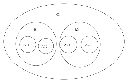
Figure 1: The structure of binary hierarchic system. The density matrix for the subsystem $A_{11}$ requires the averaging over the states of $B_{1}$ and $C_{1}$, but not over the states of $B_{2},A_{21},A_{22}$.

In general, to describe a state of an object $A_{1}$ (interacting with objects $A_{2},\ldots,A_{N}$) which is a part of an object $B_{1}$ we have to write the wave function in the form

$$\Psi=\{\psi_{B_{1}},\{\psi_{B_{1}A_{1}},\ldots,\psi_{B_{1}A_{N}}\}\},$$ (7)

where $\psi_{B_{1}}$ is the wave function of the whole (labeled by $B_{1}$), and $\psi_{B_{1}A_{1}}$ is the wave function of a component $A_{1}$ belonging to the entity $B_{1}$. For instance, $A_{1},A_{2},A_{3}$ may be quarks, and $B_{1}$ may be proton. The objects $A_{1},\ldots,A_{N}$ are inside $B_{1}$, and hence it is impossible to commute the operator-valued wave functions $[\Psi_{B_{1}},\Psi_{B_{1}A_{1}}]$ or to multiply them $\Psi_{B_{1}},\Psi_{B_{1}A_{1}}$. The functions $\Psi_{B_{1}}(x)$ and $\Psi_{B_{1}A_{1}}(x)$, taken in coordinate representation, live in different functional spaces. To label the hierarchic object (i.e. to set a coordinates on it) one needs a hierarchic tree, like those used in biology to trace the evolution. If the system $B$ consists of $k$ parts $A_{1},\ldots A_{k}$, than we can write the wave function of the form [5]:

$$|\psi\rangle=\sum C^{j}_{i_{1},\ldots,i_{k}}|\phi_{i_{1}}\rangle\otimes\ldots\otimes|\phi_{i_{k}}\rangle|\theta_{j}\rangle.$$ (8)

The equation (8) is of course an approximation, neglecting the effects of the environment $U\setminus B$. It may be considered as a kind of mean-field approximation: all effects of the environment on the subsystems $A_{k}$ are taken into account only by means of the effect of $B$ to its subsystems. Further we shall call $\phi$ the microlevel and $\theta$ the macrolevel wave function.

There are at least two aspects of the problem. First, if we know the eigenvectors $|\phi_{i_{1}}\rangle,\ldots,|\phi_{i_{k}}\rangle$ of all parts, the interaction between these parts and the effects of external fields, we should be able, in principle, to construct the set $|\theta_{j}\rangle$. But the wave functions of all constituents can’t be known simultaneously and it is more reasonable to introduce the state vector $|\theta_{j}\rangle$ of the embracing system by hand, and consider the interaction between this the mean field and the microlevel components.

Second, it is well known in biology that the action of the external fields on the components of a cell strongly depends on the state of this cell as a whole. This can be said about radiation absorption etc. Thus there is a problem of control theory. How one can control the microlevel activity acting only  on macrolevel.

Let $A$ be an operator acting on the microlevel of a system containing $k$ subparts. Then

$$\langle A\rangle=\sum{C^{*}}^{j^{\prime}}_{{i_{1}}^{\prime},\ldots,{i_{k}}^{\prime}}{C}^{j}_{{i_{1}},\ldots,{i_{k}}}\langle\theta_{j^{\prime}}|\langle\phi_{{i_{1}}^{\prime}}|\ldots\langle\phi_{{i_{k}}^{\prime}}|A|\phi_{{i_{1}}}\rangle,\ldots,|\phi_{{i_{k}}}\rangle|\theta_{j}\rangle=\rho_{\mathbf{i},\mathbf{i}^{\prime}}\langle\mathbf{i}|A|\mathbf{i}^{\prime}\rangle,$$ (9)

where $\mathbf{i}\equiv(i_{1},\ldots,i_{k}),|\mathbf{i}\rangle\equiv|\phi_{{i_{1}}}\rangle,\ldots,|\phi_{{i_{k}}}\rangle$ is the multiindex of the microlevel state.

If the operator $A=A_{1}$ acts only on the first ($i_{1}$) subsystem of the microlevel, the density matrix of this subsystem is obtained by the averaging over all other ($i_{2},\ldots,i_{k}$) subsystems and the macrosystem state

$$\rho^{(1)}_{i_{1}{i_{1}}^{\prime}}=\sum_{j,i_{2},\ldots,i_{k}}{C^{*}}^{j}_{{i_{1}}^{\prime},i_{2},\ldots,i_{k}}{C}^{j}_{{i_{1}},i_{2},\ldots,i_{k}}.$$ (10)

In analogy with the controlled gates in quantum computing algorithms, we can introduce operators which act on the microlevel depending on the state of the macrolevel [6]:

$$\hat{B}=|\mathbf{i}\rangle|\theta_{m}\rangle B^{m}_{\mathbf{i}\mathbf{k}}\langle\theta_{m}|\langle\mathbf{k}|.$$ (11)

The mean value of the corresponding observable in a two level hierarchic system is

$$\langle B\rangle=\langle\psi|\hat{B}|\psi\rangle=\sum_{j,\mathbf{i},\mathbf{i}^{\prime}}{C^{*}}^{j}_{\mathbf{i}}B^{j}_{\mathbf{i}\mathbf{i}^{\prime}}C^{j}_{\mathbf{i}^{\prime}}.$$ (12)

As an example, let us consider a system of two particles with spin $1/2$. The macrosystem of two such particles can be in either of three states: $S_{z}=0,+1,-1$. Thus a microsystem inside (say, a quark in meson) is in superposition of the states

$$|\Psi\rangle=c_{++}|\uparrow\rangle|\uparrow\rangle+c_{+0}|\uparrow\rangle|\rightarrow\rangle+c_{--}|\downarrow\rangle|\downarrow\rangle+c_{-0}|\downarrow\rangle|\rightarrow\rangle.$$ (13)

Since it is impossible for a system of spin $1$, to have $S_{z}=1$ having either of the component spins in the opposite direction, no other terms are present in the superposition (13). Taking into account the symmetry between up and down configurations, we get

$$|c_{++}|=|c_{--}|=c_{1},\quad|c_{+0}|=|c_{-0}|=c_{0}.$$

The density matrix for the subpart is

$$\rho=\left(\begin{array}[]{cc}c_{1}^{2}+c_{0}^{2}&c_{0}^{2}\\ c_{0}^{2}&c_{1}^{2}+c_{0}^{2}\end{array}\right).$$ (14)

The trace of the density matrix ${\rm}Tr(\rho)=2(c_{1}^{2}+c_{0}^{2})=1$ corresponds to the normalization of the hierarchic state (13) $\langle\Psi|\Psi\rangle=1$. Thus, measuring the state of the system by projection operator we get some information on its subsystems without acting on the subsystems wave functions. Say, if a meson is found to be in a state $|\uparrow\rangle$, then by applying the projection operator $P_{\uparrow}=|\uparrow\rangle\langle\uparrow|$ to its wave function, we get the information that both its constituent quark have the spin projections $s_{z}=\frac{1}{2}$; if meson has zero projection of spin, we can only say that its constituents have opposite projections of spins.

4 Pauli principle

It is important, that the hierarchic representation of the wave function suggests a solution to the problem, whether or not two electrons belonging to macroscopically different objects can be in the same state. By construction, the hierarchic wave functions of electrons in two different macrosystems carry the label of those macrosystems, and thus the states of the electrons are different being dependent on different labels. In fact, the solution of this problem was indicated by R.Peierls [7], who emphasized that the definition of the quantum state includes the coordinate, and since two electrons belong to different objects, they are in different states.

More formally, we can assert that two fermions belonging to the same entity of the next hierarchic level can not have coinciding quantum numbers, but those belonging to different entities of the next hierarchic level can. For instance the systems $A_{11}$ and $A_{12}$ in Fig. 1, if being fermions, can not be in the same state; but at the same time $A_{11}$ can be in the same state as $A_{21}$.

5 The Hilbert space of hierarchic states

The wave function components corresponding to different hierarchic levels may be of different nature: have different spin, isospin, color etc. and hence live in different spaces. The Hilbert space of hierarchic wave functions can be constructed by assuming common linearity at all hierarchy levels:

$$\Psi_{1},\Psi_{2}\in\mathcal{H},a,b\in\mathrm{C}\Rightarrow\Psi=a\Psi_{1}+b\Psi_{2}\in\mathcal{H}.$$

If

$$\Psi_{1} = \{\psi_{B_{1}},\{\psi_{B_{1}A_{1}},\ldots,\psi_{B_{1}A_{N}}\},\ldots\},$$

$$\Psi_{2} = \{\psi_{D_{1}},\{\psi_{D_{1}C_{1}},\ldots,\psi_{D_{1}C_{N}}\},\ldots\},$$

then their linear combination is

$$\Psi=a\Psi_{1}+b\Psi_{2}=\{a\psi_{B_{1}}+b\psi_{D_{1}},\{a\psi_{B_{1}A_{1}}+b\psi_{D_{1}C_{1}},\ldots,a\psi_{B_{1}A_{N}}+b\psi_{D_{1}C_{N}}\},\ldots\}.$$ (15)

The scalar product is defined componentwise:

$$\langle\Psi_{1}|\Psi_{2}\rangle=\langle\psi_{B_{1}}|\psi_{D_{1}}\rangle+\sum_{i=1}^{N}\langle\psi_{B_{1}A_{i}}|\psi_{D_{1}C_{i}}\rangle+\ldots.$$ (16)

The norm of the vector in hierarchic space defined by scalar product is a sum of norms of all components:

$$||\Psi||^{2}=\langle\Psi_{1}|\Psi_{1}\rangle=\langle\Psi_{B_{1}}|\Psi_{B_{1}}\rangle+\sum_{i=1}^{N}\langle\Psi_{B_{1}A_{i}}|\Psi_{B_{1}A_{i}}\rangle+\ldots.$$ (17)

The second quantization procedure can be also defined in the spaces of hierarchic states in a straightforward way. If $B$ is a system which contains the subsystems $A_{1},\ldots,A_{N}$, then the creation and annihilation operators act on the hierarchic states as follows

$$a^{+}(B)|0\rangle=|B\rangle,a(B)|B\rangle=|0\rangle,a(B)|0\rangle=0|0\rangle,$$

$$a^{+}(A_{i})|B\rangle=\{|B\rangle,|BA_{i}\rangle\},a(A_{i})\{|B\rangle,|BA_{i}\rangle\}=|B\rangle$$

$$a(B)|BA_{i}\rangle=|A_{i}\rangle.$$

Taking into account that a system is geometrically bigger then its subsystem, and therefore the step from subsystem to a system is a coarse-graining, we can see an analogy between the multiscale wave functions for an arbitrary quantum fields with the norm (17), and the decomposition of a scalar field with respect to representations of the affine group. Let $\phi(x)\in\mathrm{L}^{2}(\mathrm{R}^{d})$ be a scalar field. Using its scale components

$$\phi_{a}(b):=\int\frac{1}{a^{d/2}}\bar{\psi}\left(\frac{x-b}{a}\right)\phi(x)d^{d}x,$$

the field $\phi$ can be represented in a form of decomposition with respect to the affine group $g:x\to ax+b$:

$$\phi(x)=\frac{1}{C_{\psi}}\int\frac{1}{a^{d/2}}\psi\left(\frac{x-b}{a}\right)\phi_{a}(b)\frac{dad^{d}b}{a^{d+1}},$$ (18)

where $C_{\psi}$ is a normalization constant, which depends on the basic function $\psi$ only. The scalar product and the norm of the vector can be taken in either of representations:

$$\int|\phi(x)|^{2}dx=\int|\phi_{a}(b)|^{2}\frac{dad^{d}b}{a^{d+1}}.$$ (19)

The equation (19) is apparently a continuous counterpart of the equation (17) in case when all hierarchic components are scalar fields.

6 On sad fate of the Schrödinger Cat

The Schrödinger cats, as well as all other cats, are quantum systems with tremendous number of degrees of freedom. That’s why according to quantum mechanics the life time of any coherent superposition of such big systems is very short. In hierarchic description presented above the possibility of a superposition

$$\frac{|\hbox{``cat alive''}\rangle+|\hbox{``cat decayed into parts''}\rangle}{\sqrt{2}}$$

takes a surprising form. A hierarchic description wave function of an alive cat looks like

$$\begin{array}[]{lcl}\Psi_{\hbox{alive cat}}&=&\Bigl{\{}\psi_{cat},\left\{\psi_{cat\to head},\psi_{cat\to pams},\ldots,\psi_{cat\to tail}\right\},\ldots,\\ &&\{\psi_{cat\to head\to eye\to\ldots\to e_{-}},\ldots\},\ldots,\Bigr{\}}\end{array}.$$ (20)

In contrast, a dead cat as just “a collection of parts of the cat” (the words taken from the letter from Einstein to Heisenberg, 1950), so there should be no first term $\psi_{cat}$ (describing the entity “cat as a whole”) in the description of a dead head. The hierarchic wave function of a dead cat will look like

$$\Psi_{\hbox{dead cat}}=\Bigl{\{}\left\{\psi_{head},\psi_{pams},\ldots,\psi_{tail}\right\},\ldots,\{\psi_{head\to eye\to\ldots\to e_{-}},\ldots\},\ldots,\Bigr{\}}.$$ (21)

The hierarchic wave function of an alive cat (20) and that of dead cat (21) can not be in a superposition because they have different structure. Clearly there is now interference in the first term $\psi_{cat}+nothing$, and unlikely there is an interference in the next terms. Say, $\psi_{cat\to head}$ wave function in (20) may have different structure and much less components than $\psi_{head}$ in (21), for some of the information used to construct the head of an alive cat may have been taken from $\psi_{cat}$.

Concerning the other living beings, we dare to say that there a few characters of the living matter, which are not present in non-living matter. Namely:

1. The properties of a living system are more than just a collection of its component properties. In other words, it is impossible to predict the whole set of properties of a complex biological system even having known all properties of its components and their interactions.

2. The properties and functions of the components of a system depend on the state of the whole system. In other words, the same components being included in different systems may have different properties.

3. For a non-living matter, at least in principle, we can calculate the wave function of a big molecule by multiplying the wave functions of all the electrons and nucleons in this molecule using the Clebsh-Gordon coefficients. For a living system we can not do that, in a sense that the result of such multiplication will not give an adequate description of the system.

7 Conclusion

The understanding of physics of life and consciousness requires new mathematical methods applicable to complex systems far from equilibrium. One of the perspective approaches is the application of quantum information theory methods to biological system. Needless to say that the information theory itself often works as an ultimate tool to describe biological systems, where nonequilibrial state and strong interaction with environment precludes the application of standard quantum mechanics and thermodynamics.

In its turn, the study of biological systems by quantum mechanics and quantum information methods may be expected to yield a technical solution of the problem of long living coherent states in many-particle systems, which are so required for the construction of quantum computers, but are very likely to be present in brain [2]. The hierarchic organization of all living systems may be the key to the problem of preserving the many particle systems in a coherent superposition safe from the environmental decoherence even at room temperatures.

A mathematical framework for the description of hierarchic quantum states is presented in this paper and the previous papers [5, 6].

References

- [1] Nielsen M.A. and Chuang I.L. Quantum computation and quantum information. Cambridge University Press, 2000.
- [2] Hagan S., Hameroff, S.R. and Tuszynski, J.A. Quantum computations in brain microtubules: Decoherence and biological feasibility. Phys. Rev. E 65(2002)061901-11
- [3] Patel, A. Why genetic information processing could have a quantum basis. J.Biosciences. 26(2001)145-151; quant-ph/0105001.
- [4] Mensky M.B. Quantum measurement and decoherence. Kluver Academic, 2000.
- [5] M.V.Altaisky. What can biology bestow to quantum mechanics? pp.386-394. In Proc. Int. Cong. ”Centenary of birth of N.W.Timofeeff-Ressovsky”, Dubna, Sep 6-9, 2000. Ed. by V.I.Korogodin. JINR, Dubna, 2001.; quant-ph/0007023
- [6] M.V.Altaisky. On some algebraic problems arising in quantum mechanical description of biological systems Talk at the Int. Workshop CAAP-2001, June 28-30, 2001, Dubna, Russia; quant-ph/0110043
- [7] R.Peierls. Suprises in theoretical physics. Princeton University Press, New Jersey, 1979.