A quantitative theory-versus-experiment comparison for the intense laser dissociation of H${}_{2}^{+}$.

Abstract

A detailed theory-versus-experiment comparison is worked out for H${}_{2}^{+}$ intense laser dissociation, based on angularly resolved photodissociation spectra recently recorded in H.Figger’s group. As opposite to other experimental setups, it is an electric discharge (and not an optical excitation) that prepares the molecular ion, with the advantage for the theoretical approach, to neglect without lost of accuracy, the otherwise important ionization-dissociation competition. Abel transformation relates the dissociation probability starting from a single ro-vibrational state, to the probability of observing a hydrogen atom at a given pixel of the detector plate. Some statistics on initial ro-vibrational distributions, together with a spatial averaging over laser focus area, lead to photofragments kinetic spectra, with well separated peaks attributed to single vibrational levels. An excellent theory-versus-experiment agreement is reached not only for the kinetic spectra, but also for the angular distributions of fragments originating from two different vibrational levels resulting into more or less alignment. Some characteristic features can be interpreted in terms of basic mechanisms such as bond softening or vibrational trapping.

I Introduction

The above threshold multiphoton ionization and dissociation of H${}_{2}^{+}$ subjected to strong laser interaction, have revealed interesting nonlinear effects in angularly resolved kinetic energy distributions of the photofragments, measured in experimental works covering the last decade 1 ; 2 ; 3 ; 4 ; 5 . Among these are the observations of very large increase (or sometimes decrease) of the photodissociation rates originating from some vibrational states of the parent molecule at some specific laser intensities or, even more unexpectedly, misalignment effects in fragments angular distributions 6 . The interpretation of such behaviors has been attempted by referring to some basic dynamical mechanisms evidenced through the light-induced adiabatic potentials describing the dressed states of the molecule-plus-field system. According to the frequency regimes, bond softening (in UV) 1 ; 7 or barrier suppression (in IR) 8 mechanisms tend to enhance the dissociation cross-section especially in the polarization direction of the laser. As opposite to them vibrational trapping (in UV) 9 or dynamical dissociation quenching (in IR) 10 , act as stabilization mechanisms, favoring misalignment in the fragments distributions. This complementarity has also been referred to, for laser control purposes of the chemical reactivity; namely by softening some bonds while hardening others 11 . Although very accurate quantum calculations in the frame of time dependent approaches have been carried out, with successful interpretations of dynamical behaviors in short-intense laser pulses, to the best of our knowledge, there is no a thorough and quantitative theory-versus-experiment comparison, up to date, the work of Kondorskiy et al. Kondorskiy being a precursor in this direction. Basically two reasons can be invoked for the difficulty of such an attempt: only very few theoretical models take into account the competition between ionization and dissociation processes leading, in very strong fields, to Coulomb explosions and only very few experimental works are conducted with a careful investigation of vibrational populations and sufficiently high momentum and angular resolution yielding accurate information about the dissociation of single vibrational levels.

Experimental works on this system can be classified according to the preparation of the parent ion H${}_{2}^{+}$ from the neutral molecule H₂. A first category collects experiments referring to optical ionization with a laser prepulse 1 ; 2 ; 3 ; 4 . The independence of the ionization and dissociation processes can not be experimentally controlled, and their competition is still an open question 5 . More recently, another kind of approach has been investigated through ion beam experiments, where H${}_{2}^{+}$ ions are produced in a dc electric or plasma discharge that disentangle ionization and dissociation processes 12 ; 13 . An accelerated and strongly collimated monochromatic H${}_{2}^{+}$ beam is crossed at right angle by a focused intense laser beam. An advantage of the strong ion beam collimation is the reduction of the intensity volume effect; all ions being approximately irradiated by the same laser intensity (the validity of such approximation will however be discussed hereafter). Moreover, experiments conducted with low intensity pulses coupled to computational simulations of the resulting dissociation spectra, allow the determination of the population of the rovibrational levels of H${}_{2}^{+}$ molecules in the beam. The neutral dissociation fragments (H atoms originating from photodissociation of H${}_{2}^{+}$) are projected on a multichannel detector (MCD), whereas the charged particles (undissociated H${}_{2}^{+}$ molecules and H⁺ fragments) are extracted by deflection into a Faraday cup using an electric field. Excellent energy resolution (about 1%) allows the separation, in the circularly shaped patterns observed on the screen, the momentum projection of fragments almost originating from a single vibrational level 12 .

A model aiming in a quantitative theory-versus-experiment comparison, within the frame of the ion beam setup, has to fulfill the following requirements:

i) the photodissociation process has to be accurately described in the center of mass frame by a wavepacket propagation under the effect of an intense radiative field, starting from a given rovibrational state. There is no need, however, to refer to any competition with ionization, as the experiment precisely disentangles these two fragmentation processes.

ii) a geometrical transformation towards the MCD-plate has to be carried out, taking into account the macroscopic kinetics of the ion beam. This relates the total number of particles collected by a given pixel of the plate, during the whole experiment, to the previously calculated wavepacket, describing the evolution of an initial rovibrational state under the effect of a laser pulse of a given intensity.

iii) although particular attention has been paid to the ion beam collimation in order to reduce the field intensity volume effects, a spatial average over the laser focusing area has to be carried, taking into account the different radiative couplings felt by H${}_{2}^{+}$ molecules according to their geometrical position in the beam. This can be done through the use of some experimental measurements of the intensity distribution in the focus carried through a pinhole of 1 $\mu$m diameter 12 .

iv) quantitative agreement also requires an averaging on the detector plate using some windowing functions that simulate the resolution power of the detector.

The organization of the paper follows these achievements in Section II. The results and their interpretation are presented in Section III with a thorough discussion of the role of the intensity volume effect. An excellent theory-versus-experiment agreement is obtained not only for the kinetic but also on the angular distributions of the photofragments. Section IV is devoted to some conclusions and perspectives.

II Theory

Referring only to two radiatively coupled Born-Oppenheimer electronic states; namely the ground (1s$\sigma_{g}$) and the first excited (2p$\sigma_{u}$), an accurate wavepacket propagation method using the split operator technique is described in detail in ref.14 ; 15 . For the sake of completeness, we give hereafter a brief summary of the method, introducing the corresponding coordinates, operators and quantum numbers. The emphasis is rather put on the way to relate the quantum information content of the wavepacket to the observed momentum projections of the neutral photofragments H resulting from a rovibrational distribution of parent ions H${}_{2}^{+}$ excited by a laser source of given spatial distribution.

II.1 The wavepacket propagation

In the laboratory frame and using spherical coordinates, the total molecule-plus-field Hamiltonian is written in terms of a two-by-two operator matrix:

$$\mathbf{H}(R,\theta,\phi;t)=\mathbf{T}_{R}+\mathbf{T}_{\theta}+\mathbf{T}_{\phi}+\mathbf{V}(t).$$ (1)

$\boldsymbol{R}$ is the diatomic internuclear vector. $R$, $\theta$ and $\phi$ designate the internuclear distance, polar and azimuthal angles of $\boldsymbol{R}$ with respect to the laser polarization vector $\boldsymbol{\epsilon}$, respectively. As is usually done, a functional change on the wavepacket:

$$\boldsymbol{\Psi}(R,\theta,\phi;t)=\frac{1}{R}\boldsymbol{\Phi}(R,\theta,\phi;t)$$ (2)

aiming in a simplification of the radial part of the kinetic operators, leads to:

$$\mathbf{T}_{R}=-\mathbf{1}\frac{1}{2{\cal M}}\frac{\partial^{2}}{\partial R^{2}};$$ (3a)

$$\mathbf{T}_{\theta}=-\mathbf{1}\frac{1}{2{\cal M}R^{2}}\frac{1}{\sin\theta}\frac{\partial}{\partial\theta}\left(\sin\theta\frac{\partial}{\partial\theta}\right);$$ (3b)

$$\mathbf{T}_{\phi}=-\mathbf{1}\frac{1}{2{\cal M}R^{2}}\frac{1}{\sin^{2}\theta}\frac{\partial^{2}}{\partial\phi^{2}}$$ (3c)

with $\mathbf{1}$ the identity (2$\times$2) operator matrix. Atomic units ($\hbar$=1) are used in Eqs(3) where ${\cal M}$ designates the reduced mass. The time dependence arises in the non-diagonal terms of the potential energy operator matrix $\mathbf{V}$ through the radiative couplings:

$$V_{12}(R,\theta,t)=\mu(R)\mathcal{E}(t)\cos\theta,$$ (4)

where $\mu(R)$ is the transition dipole moment and $\mathcal{E}(t)$ is the laser electric field amplitude, given as product of a pulse shape $\epsilon(t)$ times an oscillatory term involving the carrier wave frequency $\omega$:

$$\mathcal{E}(t)=\epsilon(t)\cos\omega t.$$ (5)

Note that the $\cos\theta$ in Eq.(4) results from the dot product of the transition dipole vector (parallel to $\boldsymbol{R}$) times the laser polarization vector $\boldsymbol{\epsilon}$.

The diagonal elements $V_{1}(R)$ and $V_{2}(R)$ of $\boldsymbol{V}$ are nothing but the BO curves of the ground (label 1) and first excited (label 2) states of H${}_{2}^{+}$. $V_{1}$, $V_{2}$ and $\mu$ are obtained in the frame of the Born-Oppenheimer approximation, at the zero order level with respect to the ratio $m_{e}/m$ of the electron to the proton masses. Using spheroidal coordinates, it is well known that the Schrödinger equation can be written as two eigenvalue equations 16a ; 16b , which have been numerically solved here using the shooting method 16c . The potential energy curves have been computed in the range 0 $<R<$ 200 a.u., with a numerical accuracy checked to be better than 10^-12 a.u. The mass ratio $m/m_{e}$ has been taken as $m/m_{e}$ = 1836.152701. Finally the dipole matrix element $\mu$ between the $1s\sigma_{g}$ and $2p\sigma_{u}$ states has been obtained by numerical integration of the wave functions, at the same level of numerical accuracy.

The time dependent Schrödinger equation (TDSE) describing the wavepacket propagation is:

$$i\frac{\partial}{\partial t}\boldsymbol{\Phi}(R,\theta,\phi;t)=\mathbf{H}(R,\theta,\phi;t)\boldsymbol{\Phi}(R,\theta,\phi;t)$$ (6)

with, as an initial condition:

$$\boldsymbol{\Phi}(R,\theta,\phi;t=0)=\left(\begin{array}[]{c}\Phi_{1}(R,\theta,\phi;0)\\ 0\end{array}\right)$$ (7)

reflecting the fact that at time $t=0$, only the ro-vibrational levels of the ground electronic state are populated. The eigenfunction $\Phi_{1}$ precisely corresponds to such a state with quantum numbers $g$, $v$, $N$, $M_{N}$ (electronic ground, vibrational, total and $\boldsymbol{\epsilon}$-projected rotational) and is given by:

$$\Phi_{1}(R,\theta,\phi;0)=\chi_{g,v,N}(R)P_{N}^{M_{N}}(\cos\theta)e^{iM_{N}\phi}.$$ (8)

$P_{N}^{M_{N}}(\cos\theta)$ is the ($N$,$M_{N}$) Legendre polynomial, whereas the radial part is defined as the solution of the time-independent Schrödinger equation:

$$\left[-\frac{1}{2{\cal M}}\frac{{\mathrm{d}}^{2}}{{\mathrm{d}}R^{2}}+V_{1}(R)+\frac{N(N+1)}{2{\cal M}R^{2}}-E_{v,N}\right]\chi_{g,v,N}(E)=0.$$ (9)

The motion associated with the azimuthal angle $\phi$ remains separated under the action of the $\phi$-independent $\boldsymbol{V}$, such that $M_{N}$ is a good quantum number describing the invariance through rotation about $\boldsymbol{\epsilon}$.

The propagation using the split-operator technique has been described in full detail in previous works 14 ; 15 ; 17 . The peculiarity of odd-charged homonuclear ions is their linearly increasing dipole moment with R, leading to asymptotically divergent radiative couplings. We take them into account by splitting the wavefunction into two regions, an internal and an asymptotic one. The latter is analyzed by a generalization of the Volkov type solutions 18 , while the numerical propagation on the former is performed by Fourier transform methodology 19 with the implementation of a unitary Cayley scheme for $T_{\theta}$ 17 .

II.2 From wavepacket to observed spectra

The main concern of this paragraph is to relate the experimental observable, i.e. the probability distribution of hydrogen atoms resulting from H${}_{2}^{+}$ photodissociation, as recorded on the multichannel detector (MCD), to the asymptotic part of the wavepacket $\boldsymbol{\Phi}(R,\theta,\phi;t)$ solution of Eq.(6). By asymptotic we mean large internuclear distances $R$ for which the molecule is considered as dissociated without the possibility of a recombination process. To the best of our knowledge such a correlation has not rigorously been attempted in the literature. So far, the interpretation of general tendencies of photodissociation spectra referring to basic mechanisms, has rather been conducted by angularly resolved kinetic energy distribution given by:

$${\cal P}(k,\theta,\phi)=\lim_{t\to\infty}\left|\hat{\Phi}(k,\theta,\phi;t)\right|^{2},$$ (10)

where

$$\hat{\Phi}(k,\theta,\phi;t)=\frac{1}{\sqrt{2\pi}}\int_{-\infty}^{\infty}\Phi(R,\theta,\phi;t)e^{-ikR}{\mathrm{d}}R.$$ (11)

is the Fourier transform of $\Phi$ over the scalar variable $R$, (i.e. not over $\boldsymbol{R}$ taken as a vector). The argument retained by doing so, is that asymptotically, due to $R^{-1}$ type of behavior in the kinetic operators Eqs(3b,3c), angular dynamics is not affected at large internuclear distances. Note that in this paragraph, for the sake of simplicity, we drop the labels of $\boldsymbol{\Phi}$ depicting initial state quantum numbers ($v$, $N$, $M_{N}$).

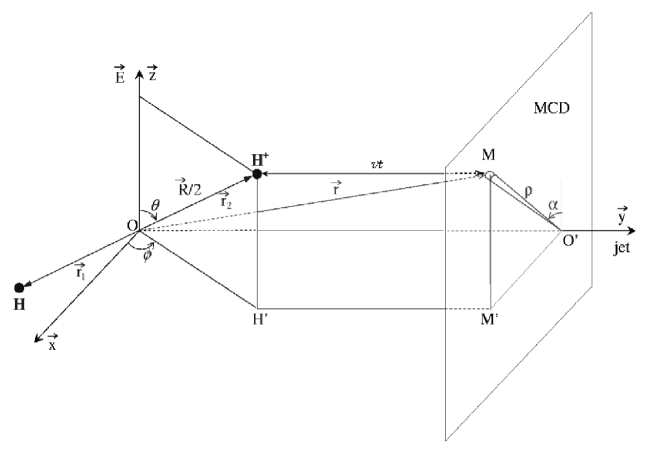
Figure 1: The H${}_{2}^{+}$ photodissociation experiment through the H₂ photoionization

To reach a comparative level of understanding, we are now describing the two families of experiments. Pertaining to the first family are photodissociation experiments where both photodissociation and photoionization steps are laser induced 1 ; 2 ; 3 ; 4 . Starting from neutral H₂, in its ground electronic and vibrationless state X($v$=0), a multiphoton excitation leads, through the EF intermediate excited electronic state, to the H${}_{2}^{+}$ ground state with a distribution of rovibrational levels. Dissociation follows the absorption of additional photons and is very fast as compared to the relative motion of the parent ion H${}_{2}^{+}$ in the laboratory frame. Whence the photofragments are well separated, H⁺ ions are extracted (accelerated) through an electric field and collected on the MCD plate. A schematic view is provided in figure 1. Photodissociation occurs, as a fast process, at the origin $O$ of the laboratory frame, at a time which is taken as $t=0$. The laser polarization vector is along the $z$-direction, $\boldsymbol{r_{1}}$ and $\boldsymbol{r_{2}}$ are the vectors pointing H and H⁺. A further step is the extraction of the proton H⁺ by an electric field applied along the $\boldsymbol{y}$-direction towards the MCD plate positioned at a distance $OO^{\prime}$=$D$ from the origin. The detection occurs on a pixel $M$ defined by its polar coordinates ($\rho$, $\alpha$) on the MCD surface (or by $\boldsymbol{r}$ with respect to $O$) that H⁺ is reaching after a time of flight $t$, with velocity $v$. It is worthwhile noting that this last step is just a mapping of the photofragment onto the detector (without dissociation during time $t$). The vector transformation relating the proton H⁺ position ($R,\theta,\phi$) in the center of mass frame to the pixel M ($\rho,\alpha$) on the detector is known as the Abel transformation 23 .

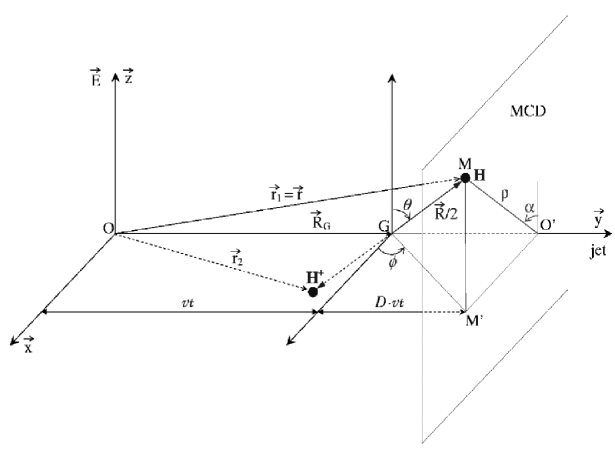
Figure 2: The H${}_{2}^{+}$ photodissociation experiment based on the ionization of H₂ using discharge source

A different situation prevails in the experiments of the second family where an electric or a plasma discharge ionizes H₂ into H${}_{2}^{+}$ 12 ; 13 . The resulting ion beam is strongly accelerated by an electric field and is crossed at $t=0$ by the laser beam at a point $O$ of the laboratory frame. The description of such experiments, as illustrated in figure 2, has to combine two motions; namely, the translation of the center of mass $G$ in the laboratory frame along $\boldsymbol{u_{y}}$ (unit vector along $\boldsymbol{y}$) with velocity $v$ and the nuclear separation (dissociation) in the center of mass frame. The hydrogen atom H resulting from photofragmentation is collected at the pixel $M$ of the detector. It is to be noted that $M$ is positioned with respect to the laboratory frame with a vector $\boldsymbol{r}$, corresponding to $\boldsymbol{r_{1}}$ at time $t$, when H reaches $M$.

As, our concern is the quantitative interpretation of photodissociation spectra obtained in H.Figger’s group using an electric discharge to induce ionization 12 ; 20 ; 21 , emphasis is put in the following on a thorough description of the kinematics of the second family experiments. The quantity which is measured, is nothing but the number of hydrogen atoms ${\mathrm{d}}N$ collected on each pixel $M$ ($\rho$, $\alpha$) at infinite time. This can ultimately been related with the time integral of the flux of the current density $\boldsymbol{j}(\rho,\alpha,t)$ of H orthogonal to the area ${\mathrm{d}}S=\rho{\mathrm{d}}\rho{\mathrm{d}}\alpha$ of the finite size pixel $M$, as

$${\mathrm{d}}N(\rho,\alpha)=N{\mathrm{d}}S\int_{0}^{\infty}\boldsymbol{j}(\rho,\alpha,t)\cdot\boldsymbol{u_{y}}{\mathrm{d}}t,$$ (12)

where $N$ is the total number of H photofragments. The flux in Eq.(12), involves an averaging over the positions of all protons H⁺ that are not detected in the experiment 125 :

$$\boldsymbol{j}(t)=\frac{1}{m}\int{\mathrm{d}}\boldsymbol{r_{2}}\ \mathrm{Im}\left[\Psi^{*}(\boldsymbol{R},\boldsymbol{R_{G}};t)\nabla_{\boldsymbol{r_{1}}}\Psi(\boldsymbol{R},\boldsymbol{R_{G}};t)\right].$$ (13)

where $\Psi(\boldsymbol{R},\boldsymbol{R_{G}};t)$ is the overwhole wavepacket describing the combined molecular internal $\boldsymbol{R}$-motion and center of mass $\boldsymbol{R_{G}}$-motion. $\mathrm{Im}$ stands for the imaginary part. Frame transformations defining $\boldsymbol{R_{G}}$ and some vector relations directly related with figure 2, are gathered in an Appendix. Separation of the photofragments relative motion described by $\Psi(\boldsymbol{R};t)$, from the motion of the center of mass described by $\Phi_{G}(\boldsymbol{R_{G}};t)$, leads to the following representation of the total wavefunction:

$$\Psi(\boldsymbol{R},\boldsymbol{R_{G}};t)=\Psi(\boldsymbol{R};t)\Phi_{G}(\boldsymbol{R_{G}};t).$$ (14)

Using the frame transformations Eqs(A-1,A-2) together with Eq.(2) one has:

$$\Psi(\boldsymbol{R},\boldsymbol{R_{G}};t)=\frac{\Phi(\boldsymbol{r_{1}}-\boldsymbol{r_{2}};t)}{||\boldsymbol{r_{1}}-\boldsymbol{r_{2}}||}\Phi_{G}\left(\frac{(\boldsymbol{r_{1}}+\boldsymbol{r_{2}})}{2};t\right).$$ (15)

Concerning the calculation of the gradient $\nabla_{\boldsymbol{r_{1}}}$ involved in Eq.(13), we note that the flux has to be evaluated at large $R$ with as consequences:

$$\nabla_{\boldsymbol{r_{1}}}\Phi(\boldsymbol{R};t)=\nabla_{\boldsymbol{R}}\Phi(\boldsymbol{R};t)\simeq\boldsymbol{u_{R}}\frac{\partial}{\partial R}\Phi(\boldsymbol{R};t)$$ (16)

with $\boldsymbol{u_{R}}$ the unit vector along $\boldsymbol{R}$ (Eq.(A-6)) and

$$\nabla_{\boldsymbol{r_{1}}}\Phi_{G}(\boldsymbol{R_{G}};t)=\frac{1}{2}\nabla_{\boldsymbol{R_{G}}}\Phi_{G}(\boldsymbol{R_{G}};t)$$ (17)

The approximation involved in Eq.(16) results from the neglect of all angular derivations due to their occurrence with coefficients decreasing faster than $R^{-1}$. We proceed now to a quasiclassical approximation for the description of the center of mass translational motion, with two implications:

(i) $\boldsymbol{R_{G}}\simeq v\boldsymbol{u_{y}}t$ has a corresponding wavevector $\boldsymbol{K_{G}}\simeq mv\boldsymbol{u_{y}}$ and the application of momentum operator $-i\nabla_{\boldsymbol{R_{G}}}$ to $\Phi_{G}(\boldsymbol{R_{G}})$ simply result into $mv\Phi_{G}(\boldsymbol{R_{G}})$. When this is done at the level of Eq(13) one gets:

$$\boldsymbol{j}(t)=\frac{1}{m}\int d\boldsymbol{r_{2}}\frac{1}{|\boldsymbol{r_{1}}-\boldsymbol{r_{2}}|^{2}}\mathrm{Im}\left[\Phi^{*}(\boldsymbol{R};t)\frac{\partial}{\partial R}\Phi(\boldsymbol{R};t)+imv|\Phi(\boldsymbol{R};t)|^{2}\right]|\Phi_{G}(\boldsymbol{R_{G}};t)|^{2}.$$ (18)

(ii) No wavepacket spreading is allowed for $\Phi_{G}(\boldsymbol{R_{G}};t)$ which is localized with an envelope behaving as a $\delta$-like function, i.e.:

$$|\Phi_{G}(\boldsymbol{R_{G}})|^{2}\simeq\delta(R_{G}-vt).$$ (19)

The integration over $\boldsymbol{r_{2}}$ (with ${\mathrm{d}}\boldsymbol{r_{2}}=2{\mathrm{d}}\boldsymbol{R_{G}}$) finally leads to:

$$\boldsymbol{j}(t)=\frac{1}{mR^{2}}\mathrm{Im}\left.\left[\Phi^{*}(\boldsymbol{R};t)\frac{\partial}{\partial R}\Phi(\boldsymbol{R};t)\boldsymbol{u_{R}}+imv|\Phi(\boldsymbol{R};t)|^{2}\boldsymbol{u_{y}}\right]\right|_{\boldsymbol{R}=2\boldsymbol{r_{1}}-2vt\boldsymbol{u_{y}}},$$ (20)

with a rather intuitive interpretation of the two components of the flux. The first ı.e. $\Phi^{*}(\boldsymbol{R};t)\frac{\partial}{\partial R}\Phi(\boldsymbol{R};t)\boldsymbol{u_{R}}$ is merely the current density generated by the expanding wavepacket in the center of mass frame, whereas the second corresponds to the current associated with a density $\frac{|\Phi|^{2}}{R^{2}}$ travelling with a velocity $v$ along $\boldsymbol{u_{y}}$. The calculation can be further conducted analytically by deriving an asymptotic (i.e. $R\to\infty$, $t\to\infty$) expression for $\Phi$ 126 . This is done using a time evolution expression involving the Fourier transform Eq.(11). Actually, one has for large $R$, where the potentials can be considered as constant and after the laser is turned off:

$$\hat{\Phi}(k,\theta,\phi;t)=e^{-ik^{2}t/m}\hat{\Phi}(k,\theta,\phi)$$ (21)

the solution being induced only by the radial part of the kinetic energy. Returning back to the wavepacket in the coordinate space:

$$\Phi(R,\theta,\phi;t)=\frac{1}{\sqrt{2\pi}}\int_{-\infty}^{\infty}{\mathrm{d}}k\hat{\Phi}(k,\theta,\phi)e^{-ik^{2}t/m}e^{ikR}$$ (22)

and replacing $\hat{\Phi}$ by its expression Eq.(11), one gets:

$$\Phi(R,\theta,\phi;t)=\left(\frac{m}{4i\pi t}\right)^{1/2}\int_{0}^{\infty}{\mathrm{d}}R^{\prime}\Phi(R^{\prime},\theta,\phi)e^{im(R-R^{\prime})^{2}/4t}.$$ (23)

Expanding the $R$-dependent part of the exponential as:

$$e^{\frac{im}{4t}(R-R^{\prime})^{2}}=e^{\frac{imR^{2}}{4t}}e^{-\frac{imRR^{\prime}}{2t}}\left[1+\left(e^{\frac{im{R^{\prime}}^{2}}{4t}}-1\right)\right]$$ (24)

and observing 22 that for large $t$:

$$\lim_{t\to\infty}\left|\left(e^{\frac{im{R^{\prime}}^{2}}{4t}}-1\right)\right|=0,$$ (25)

an asymptotic expression is obtained for $\Phi(R,\theta,\phi;t)$:

$$\Phi(R,\theta,\phi;t)\sim_{t\to\infty}\left(\frac{m}{2it}\right)^{1/2}e^{\frac{imR^{2}}{4t}}\hat{\Phi}\left(\frac{mR}{2t},\theta,\phi\right).$$ (26)

While recasting Eq.(26) into Eq.(20), a rather simple expression results for the asymptotic flux:

$$\boldsymbol{j}(t)=\frac{m}{2Rt^{2}}\left.\left[\boldsymbol{u_{R}}+\frac{2vt}{R}\boldsymbol{u_{y}}\right]\left|\hat{\Phi}\left(\frac{mR}{2t},\theta,\phi\right)\right|^{2}\right|_{\boldsymbol{R}=2(\boldsymbol{r_{1}}-vt\boldsymbol{u_{y}})}$$ (27)

The calculation of the projection of $\boldsymbol{j}$ on $\boldsymbol{u_{y}}$ (cf Eq.12) requires the vector relation of Eq.(A-7) that finally leads to:

$$\boldsymbol{j}\cdot\boldsymbol{u_{y}}=\frac{mD}{4t^{2}}\frac{1}{[\rho^{2}+(D-vt)^{2}]^{2}}\left|\hat{\Phi}\left(\frac{mR}{2t},\theta,\phi\right)\right|^{2}.$$ (28)

where $R$ depends on $t$ as given by Eq.(A-3).

The final step is to transform the time integration of $\boldsymbol{j}\cdot\boldsymbol{u_{y}}$, involved in Eq.(12), into an integration over the kinetic momentum. We proceed to a change of variable:

$$k=[\rho^{2}+(D-vt)^{2}]^{1/2}\frac{mv}{D}=\frac{R}{2}\frac{mv}{D},$$ (29)

the physical meaning of which will be clarified hereafter. Straightforward calculations show that Eq.(29) can be inverted as:

$$t=\left\{\begin{array}[]{l}\frac{D}{v}\left(1-\frac{(k^{2}-k_{\rho}^{2})^{1/2}}{mv}\right)\ \ \mathrm{for}\ t\in\left[0,\frac{D}{v}\right]\ \ (k\in[k_{\rho},(k_{\rho}^{2}+m^{2}v^{2})^{1/2}])\\ \frac{D}{v}\left(1+\frac{(k^{2}-k_{\rho}^{2})^{1/2}}{mv}\right)\ \ \mathrm{for}\ t\in\left[\frac{D}{v},+\infty\right]\ \ (k\in[k_{\rho},+\infty])\\ \end{array}\right.,$$ (30)

upon the introduction of the notation

$$k_{\rho}=mv\frac{\rho}{D}$$ (31)

and leads to:

$${\mathrm{d}}t=\mp\frac{D}{mv^{2}}\frac{k}{\left(k^{2}-k_{\rho}^{2}\right)^{1/2}}{\mathrm{d}}k.$$ (32)

The $\mp$ signs correspond to the two time intervals depicted in Eqs(30). The time dependent argument of $\hat{\Phi}$ in Eq.(26) can than be expressed using the two variables $k$ (Eq.(29)) and $k_{\rho}$ (Eq.(31)) as:

$$\frac{mR}{2t}=\frac{m}{t}[\rho^{2}+(D-vt)^{2}]^{1/2}=\frac{D}{vt}k=k\left(1\mp\frac{(k^{2}-k_{\rho}^{2})^{1/2}}{mv}\right)^{-1}.$$ (33)

The experimental conditions, are such that the velocity $v$ of the molecular beam is much greater than the fragments relative velocity. We can thus consider $(k^{2}-k_{\rho}^{2})^{1/2}/mv$ as negligible when compared to 1, taking into account that $D$ is much larger than $\rho$. The resulting approximation, namely:

$$t\simeq\frac{D}{v}\ \ \ \ {\mathrm{a}nd}\ \ \ \ \frac{mR}{2t}\simeq k$$ (34)

merely means that the time needed for a fragment to reach the pixel $M(\rho,\alpha)$ is approximately the same as the one needed for the center of mass $G$ to reach the center $O^{\prime}$ of the detector. In the framework of this approximation, the meaning of $k_{\rho}=m\rho v/D\simeq m\rho/t$ (defined by Eq.(31) ) is also clear: i.e. the projection of the kinetic momentum $k$ on the detector plane. Finaly we obtain for the time integrated flux:

$$\int_{0}^{\infty}\boldsymbol{j}\cdot\boldsymbol{u_{y}}{\mathrm{d}}t=\frac{m^{2}v^{2}}{4D^{2}}\left[\int_{k\rho}^{\infty}+\int_{k\rho}^{(k_{\rho}^{2}+m^{2}v^{2})^{1/2}}\frac{\left|\hat{\Phi}\left(k,\theta,\phi\right)\right|^{2}}{k\left(k^{2}-k_{\rho}^{2}\right)^{1/2}}{\mathrm{d}}k\right]$$ (35a)

$$=\frac{m^{2}v^{2}}{2D^{2}}\int_{k\rho}^{\infty}\frac{\left|\hat{\Phi}\left(k,\theta,\phi\right)\right|^{2}}{k\left(k^{2}-k_{\rho}^{2}\right)^{1/2}}{\mathrm{d}}k.$$ (35b)

where the upper bond of the second integral in Eq.(35a) has been extended up to $+\infty$ considering that $|\hat{\Phi}(k,\theta,\phi)|=0$ for $k>mv$, which is equivalent to state that the center of mass kinetic momentum $2mv$ is much larger than the relative momentum of photofragments $k$. Recasting Eqs(35) in Eq.(12), taking into account cylindrical symmetry over $\phi$ and calculating the pre-integral factor as:

$$\frac{m^{2}v^{2}}{D^{2}}{\mathrm{d}}S=\frac{mv\rho}{D}\frac{mv{\mathrm{d}}\rho}{D}{\mathrm{d}}\alpha=k_{\rho}{\mathrm{d}}k_{\rho}{\mathrm{d}}\alpha.$$ (36)

one finally gets:

$${\mathrm{d}}N(k_{\rho},\alpha)=Nk_{\rho}{\mathrm{d}}k_{\rho}{\mathrm{d}}\alpha\frac{1}{2}\int_{k_{\rho}}^{\infty}\frac{\left|\hat{\Phi}\left(k,\theta\right)\right|^{2}}{k\left(k^{2}-k_{\rho}^{2}\right)^{1/2}}{\mathrm{d}}k.$$ (37)

The dependence over $\theta$ of the right-hand-side of Eq.(37) has to be expressed in terms of $\alpha$, referring to the frame transformation Eq.(A-9)

$$\cos\theta=\frac{k_{\rho}}{k}\cos\alpha$$ (38)

in such a way that, ultimately ${\mathrm{d}}N$ is written only in terms of the variables $k_{\rho}$ and $\alpha$, with the parameters $v$ and $D$ characterizing the experimental setup:

$${\mathrm{d}}N(k_{\rho},\alpha)=Nk_{\rho}{\mathrm{d}}k_{\rho}{\mathrm{d}}\alpha\frac{1}{2}\int_{k_{\rho}}^{\infty}\frac{\left|\hat{\Phi}\left(k,\arccos(k_{\rho}/k\cos\alpha)\right)\right|^{2}}{k\left(k^{2}-k_{\rho}^{2}\right)^{1/2}}{\mathrm{d}}k.$$ (39)

The probability to record a hydrogen atom on the surface element $\mathrm{d}S$ (pixel $M$) located at $\rho$, $\alpha$ on the MCD (with a kinetic momentum $k_{\rho}$) is obtained by a proper normalization:

$$P(k_{\rho},\alpha){\mathrm{d}}S=\frac{1}{N}{\mathrm{d}}N(k_{\rho},\alpha)=\frac{{\mathrm{d}}S}{2}\int_{k_{\rho}}^{\infty}\frac{\left|\hat{\Phi}\left(k,\arccos(k_{\rho}/k\cos\alpha)\right)\right|^{2}}{k\left(k^{2}-k_{\rho}^{2}\right)^{1/2}}{\mathrm{d}}k.$$ (40)

It is interesting to note that the two probabilities ${\cal P}(k,\theta)$ (given in Eq.10) and $P(k_{\rho},\alpha)$ (Eq.(40)) are simply connected by:

$$P(k_{\rho},\alpha)=\frac{1}{2}\int_{k_{\rho}}^{\infty}\frac{{\cal P}(k,\theta)}{k\left(k^{2}-k_{\rho}^{2}\right)^{1/2}}{\mathrm{d}}k.$$ (41)

Two remarks are in order:

i) both equations Eq.(40) and Eq.(41) involve a singularity at $k=k_{\rho}$. This difficulty can be overcame by a partial integration leading to:

$$\begin{split}P(k_{\rho},\alpha)=\frac{1}{2k_{\rho}}\arccos\left(\frac{k_{\rho}}{k}\right){\cal P}\left(k,\theta\right)\Big{|}_{k=k{\rho}}^{k=\infty}-\frac{1}{2k_{\rho}}\int_{k_{\rho}}^{\infty}\arccos\left(\frac{k_{\rho}}{k}\right)\frac{{\mathrm{d}}}{{\mathrm{d}}k}{\cal P}(k,\theta){\mathrm{d}}k\end{split}$$ (42)

The integrated term in the right-hand-side of Eq.(42) is null, due to the fact that ${\cal P}(k,\theta)\Big{|}_{k=\infty}=0$. As for the total derivative with respect to $k$ of ${\cal P}(k,\theta)$, it results into:

$$\begin{split}\frac{{\mathrm{d}}}{{\mathrm{d}}k}{\cal P}(k,\theta)=\frac{\partial{\cal P}}{\partial k}+\frac{k_{\rho}\cos\alpha}{k(k^{2}-k_{\rho}^{2}\cos^{2}\alpha)^{1/2}}\frac{\partial{\cal P}}{\partial\theta}.\end{split}$$ (43)

When recasting Eq.(43) into Eq.(42) one obtains:

$$\begin{split}P(k_{\rho},\alpha)=-\frac{1}{2k_{\rho}}\int_{k_{\rho}}^{\infty}\arccos\left(\frac{k_{\rho}}{k}\right)\left[\frac{\partial{\cal P}}{\partial k}+\frac{k_{\rho}\cos\alpha}{k(k^{2}-k_{\rho}^{2}\cos^{2}\alpha)^{1/2}}\frac{\partial{\cal P}}{\partial\theta}\right]{\mathrm{d}}k\end{split}$$ (44)

For $k\simeq k_{\rho}$, the singularity in the coefficient of $\frac{\partial{\cal P}}{\partial\theta}$ may only occur for $\alpha=0$. This is fortunately compensated by the $\arccos(k_{\rho}/k)$ term of Eq.(42). Actually expanding Eq.(42) in terms of powers of $(1-k_{\rho}/k)$ one ends up with a non-singular behavior, i.e. $\frac{1}{k_{\rho}}\frac{\partial{\cal P}}{\partial\theta}$ for the integrand in the vicinity of $k_{\rho}$.

ii) Despite the fact that the experimental situation we are describing is not amenable to a simple mapping on the detector plate of a photodissociation that had already occured in the center of mass frame (as a figure 1), it turns out that Eq.(40) can finally be recast in terms of the commonly used Abel transformation 225 :

$$P(k_{\rho},\alpha)=\frac{1}{4}{\cal A}\left[\left|\frac{\hat{\Phi}\left(k,\arccos(k_{\rho}/k\cos\alpha)\right)}{k}\right|^{2}\right],$$ (45)

where $\cal A$ is defined as 225 :

$${\cal A}[f(k)](x)=2\int_{x}^{\infty}\frac{f(k)k}{\left(k^{2}-x^{2}\right)^{1/2}}{\mathrm{d}}k.$$ (46)

In connection with this, it is worthwhile considering the full Fourier transform of the wavefunction describing the relative motion (in contrast to the one carried in Eq.11):

$$\hat{\Psi}(\boldsymbol{k})=\frac{1}{(2\pi)^{3/2}}\int\!\!\!\int\!\!\!\int{\mathrm{d}}\boldsymbol{R}\Psi(\boldsymbol{R})e^{-i\boldsymbol{k}\boldsymbol{R}}$$ (47)

It can be shown by following the same derivations as Eqs(21-26) 126 ; 22 , that asymptotically (i.e. for $t\to+\infty$ and $R\to+\infty$), one has:

$$\Psi(\boldsymbol{R};t)=\left(\frac{m}{2it}\right)^{3/2}e^{-imR^{2}/4t}\hat{\Psi}\left(\frac{m\boldsymbol{R}}{2t}\right)$$ (48)

which, combined with Eqs(2 and 26), implies that:

$$|\hat{\Psi}(\boldsymbol{k};t)|^{2}=\left|\frac{\hat{\Phi}(\boldsymbol{k};t)}{k}\right|^{2},$$ (49)

The probability in Eq.(45) appears now as the Abel transform of $\left|\hat{\Psi}\left(k,\arccos(k_{\rho}/k\cos\alpha)\right)\right|^{2}$.

II.3 Rovibrationally averaged spectra

The probability distributions which are calculated in the previous paragraph refer to a given initial state ($g$, $v$, $N$, $M_{N}$) involved in the determination of $\Phi(t=0)$ through Eq.(8) such that the quantity resulting from Eq.(45) is actually $P_{v,N,M_{N}}(k_{\rho},\alpha)$ using a full notation. An averaging over the initial ro-vibrational populations is thus required to reach the experimental spectra. As the rotational states $N$ are $(2N+1)$ times degenerated, a summation can be carried out over $M_{N}$, leading to:

$$P_{v,N}(k_{\rho},\alpha)=\frac{1}{2N+1}\sum_{M_{N}=0}^{N}c_{M_{N}}P_{v,N,M_{N}}(k_{\rho},\alpha),$$ (50)

where $c_{0}=1$ and $c_{M_{N}}=2$ (for $M_{N}\neq 0$), due to the fact that the total Hamiltonian does not depend upon the sign of $M_{N}$. The homonuclear diatomic character of H${}_{2}^{+}$ implies a total wavefunction (accounting for the nuclear spin) that is antisymmetric with respect to the interchange of identical nuclei. To ensure such a property the total nuclear spin number $T$ must be either $0$ (associated with even $N$), or $1$ (associated with odd $N$). Due to very rare singlet ($T=0$) - triplet ($T=1$) transitions, molecular hydrogen mainly consists of two distinct species: parahydrogen ($T=0$) and orthohydrogen ($T=1$). The occurrence of ortho states is three times more probable than the para ones 14 . This nuclear spin statistics is accounted for, by a weighting coefficient $g_{N}$, affecting the rotational populations $N$, such that

$$g_{N}=\left\{\begin{array}[]{c}1\textrm{ for even }N\\ 3\textrm{ for odd }N\end{array}\right.$$ (51)

Apart from this factor, rotational populations are also thermally weighted, according to a Boltzman distribution described by a rotational temperature $T_{v}$ depending on the initial vibrational level. The weighting coefficient is given by:

$$b_{N}=\exp\left[-\frac{\Delta E(v,N)}{k_{\beta}T_{v}}\right].$$ (52)

where $k_{\beta}$ stands for the Boltzman constant and $\Delta E(v,N)$ for the rotational energies resulting from the solution of Eq.(9):

$$\Delta E(v,N)=E(v,N)-E(v,0).$$ (53)

The rotationally averaged probabilities resulting from these considerations are

$$P_{v}(k_{\rho},\alpha)=\frac{1}{Q_{v}}\sum_{N}b_{N}g_{N}P_{v,N}(k_{\rho},\alpha),$$ (54)

where $Q_{v}$ is a normalization factor:

$$Q_{v}=\sum_{N}b_{N}g_{N}.$$ (55)

The comparison with experimental spectra has also to take into account initial vibrational populations $a(v)$ (i.e. as they result from the electric discharge acting over H₂, prior to the laser excitation):

$$P(k_{\rho},\alpha)=\frac{1}{Q}\sum_{v}a(v)P_{v}(k_{\rho},\alpha),$$ (56)

with

$$Q=\sum_{v}a(v).$$ (57)

We note that the informations concerning the initial vibrational distribution $a(v)$ as well as the corresponding rotational temperature $T_{v}$, have to be provided by experimental measurements.

II.4 Laser spatial intensity averaging

Although particular attention is devoted in the experimental measurements for obtaining a well focussed ion beam, the molecules are actually excited by different field amplitudes according to their positions ($x$, $y$), due to a non-homogeneous spatial intensity distribution $I(x,y)$ in the laser beam. It turns out that an average over these non-homogeneities has a basic importance when attempting a quantitative interpretation of experimental data, as will be clear in the next section. The average implies a double spatial integration over the variables $x$ and $y$ (see figure 6):

$$P(k_{\rho},\alpha)=\int_{-L}^{L}dx\int_{-\infty}^{+\infty}P(k_{\rho},\alpha;I(x,y))dy.$$ (58)

$x$ being limited to a finite interval $2L$ measuring the width of the ion beam. The integrand itself is nothing but the probability calculated in Eq.(56) with as an additional argument the intensity $I(x,y)$, for which this probability is calculated, i.e. $P(k_{\rho},\alpha;I(x,y))$. For parity reasons Eq.(58) may be also written as:

$$P(k_{\rho},\alpha)=4\int_{0}^{L}dx\int_{0}^{+\infty}P(k_{\rho},\alpha;I(x,y))dy.$$ (59)

A gaussian shape is assumed for the 2D behavior of the laser within its focus area:

$$I(x,y)=I_{0}\exp\left[-\frac{x^{2}}{r_{x}^{2}}\right]\exp\left[-\frac{y^{2}}{r_{y}^{2}}\right]$$ (60)

where $r_{x}$ and $r_{y}$ are the radii of the focal area, such that $I(r_{x},r_{y})=I_{0}/e^{2}$. These parameters are obtained from the experimental setup 12 as:

$$r_{x,y}=\frac{\lambda f}{2\pi b_{x,y}}$$ (61)

where $\lambda$ is the laser wavelength and $f$ is the focal length of the parabolic mirror focusing the laser beam. $b_{x}$ and $b_{y}$ correspond to the extensions in each direction $x$ and $y$ where 50% of the energy is dissipated. The peak intensity is calculated whence the total pulse energy $E_{0}$ and an autocorrelation time $t_{ac}$ have been measured:

$$I_{0}=\frac{2\sqrt{2\ln 2}E_{0}}{\pi^{3/2}r_{x}r_{y}t_{ac}}.$$ (62)

The double integration involved in Eq.(59) can be conducted, by integrating first over $y$, referring to a variable change:

$$y=r_{y}\left[-\ln\left(\frac{I}{I_{x}}\right)\right]^{1/2}$$ (63a)

$$dy=-\frac{r_{y}}{2}\left[-\ln\left(\frac{I}{I_{x}}\right)\right]^{-1/2}\frac{dI}{I},$$ (63b)

where $I_{x}=I_{0}\exp\left[-(x/r_{x})^{2}\right]$. The result is:

$$P(k_{\rho},\alpha;I_{x})=2r_{y}\int_{0}^{I_{x}}\frac{P(k_{\rho},\alpha;I)}{I\left[-\ln\left(\frac{I}{I_{x}}\right)\right]^{1/2}}dI.$$ (64)

Two singularities affect such an expression; namely at $I=0$ and at $I=I_{x}$. The first has no consequence, as for $I=0$, $P(k_{\rho},\alpha;I=0)=0$. The second can be avoided when integrating by part:

$$P(k_{\rho},\alpha;I_{x})=2r_{y}\left[-2\sqrt{I/I_{x}}P(k_{\rho},\alpha;I)+\int_{0}^{I_{x}}2\sqrt{I/I_{x}}\frac{d}{dI}P(k_{\rho},\alpha;I)dI\right]$$ (65)

An identical procedure is then applied for the second integral over $x$. The final result is

$$P(k_{\rho},\alpha)=2r_{x}\left[\left.-2\sqrt{I_{x}/I_{0}}P(k_{\rho},\alpha;I_{x})\right|^{I_{x}=I_{0}}_{I_{x}=I_{L}}+\int_{I_{L}}^{I_{0}}2\sqrt{I_{x}/I_{0}}\frac{d}{dI_{x}}P(k_{\rho},\alpha;I_{x})dI_{x}\right]$$ (66)

where $I_{L}$ is the field intensity at ($x=L$, $y=0$).

III Results

This section presents the results of the simulation and interpretation of experimental data. Among the experimental results obtained in H.Figger’s group 12 ; 20 ; 21 three are retained. The laser intensities $I_{0}$ have been slightly adjusted with respect to laboratory measurements of the total pulse energy $E_{0}$ and autocorrelation time $t_{ac}$, to fit experimental spectra. The resulting parameters are collected in Table 1. The laser pulse carrier wavelength is $\lambda$=785 nm.

E0 (mJ)	tac (fs)	I0 (TW/cm2)
0.3	228	7.5
0.5	234	9.5
0.7	240	16.0

Table 1: Total pulse energy E₀ and autocorrelation time t_ac of the laser field. $I_{0}$ is the maximal field intensity value.

In the calculations the intensity spatio-temporal distribution is assumed to be:

$$I(x,y;t)=I_{0}\exp\left[-\frac{x^{2}}{r_{x}^{2}}\right]\exp\left[-\frac{y^{2}}{r_{y}^{2}}\right]\exp\left[-\frac{2t^{2}}{w_{t}^{2}}\right]$$ (67)

with the relations between the parameters as given by Eqs(61, 62). The widht of the molecular jet is $L$=50 $\mu$m, its velocity is $v$=10⁶ m/s and focal area parameters values are $b_{x}$=2.6 mm, $b_{y}$=2.4 mm, $f$=1000 mm, resulting into $r_{x}$=48$\mu$m, $r_{y}$=52$\mu$m. In the calculations described below the parameter $w_{t}=t_{ac}/2\sqrt{ln2}$, which define the laser pulse temporal shape, have been taken equal to 140 fs.

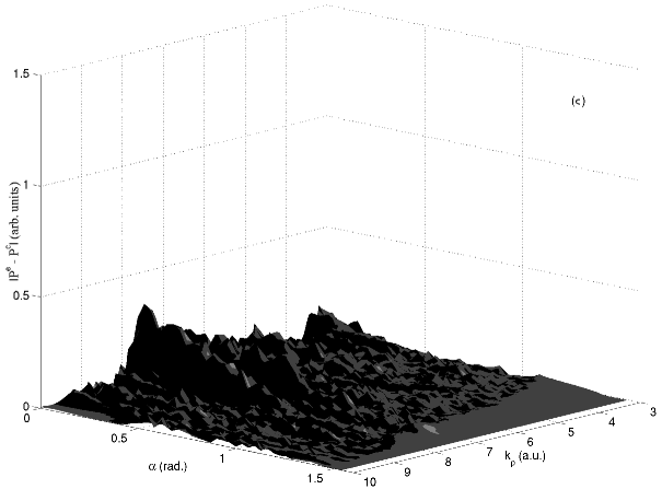
Figure 3: (a) - The three dimensional representation of the experimental result corresponding to E₀=0.7 mJ (see the third line in Tab.(1); (b) - The corresponding calculation result; (c) - The difference between experimental and calculated spectra.

Figure 3 displays three-dimensional representations of the dissociation probabilities as a function of their angular ($\alpha$) and kinetic ($k_{\rho}$) distributions. The upper diagram corresponds to the experimental results $P^{e}$ 20 for the laser excitation parameters indicated on the last row of Table 1. The lowest two diagrams give the calculated spectrum ($P^{c}$) and the absolute value of the difference $\left|P^{e}-P^{c}\right|$, for the same laser characteristics, at the same scale. The normalization is such that:

$$\int_{0}^{\infty}k_{\rho}dk_{\rho}\int_{0}^{\pi/2}P^{e,c}(k_{\rho},\alpha)d\alpha=1.$$ (68)

The successive peaks that are obtained correspond to photofragments arising from different vibrational levels $v$ of the parent ion H${}_{2}^{+}$. The energies of the levels are positioned in figure 4 on the rotationless dressed molecular potentials resulting from the diagonalization of the radiative interaction at fixed angle $\theta=0$.

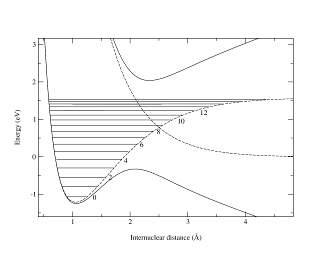
Figure 4: 2D view of the dressed adiabatic potential curves of H${}_{2}^{+}$ (solid lines) (with a continuous wave laser of wavelength $\lambda$=785 nm and intensity $I_{0}$=1.6$\times$10¹³ W/cm²) and the corresponding diabatic BO electronic states (dashed lines). Are also indicated the eigenvalues of the field-free vibrational levels.

The most important peak (at $\alpha=0$) corresponds to $v$=7 and is followed in decreasing order by the peaks assigned to $v$=8,9,10. The peak resulting from the dissociation of $v$=6, with a much smaller contribution is hidden by the peak $v$=7, whereas those resulting from $v$=11,12 are in the blue-wing of $v$=10. It is interesting to note that, on the lowest diagram, the largest error affects the peak resulting from v=9, all others being well represented. This is to be relationed with the particular energy of $v$=9 (see figure 4) very close to the avoided crossing of the dressed potentials. The characteristics of this region being very sensitive to the laser spatial and temporal intensity distributions, even small deviations with respect to experimental evaluations may lead to appreciable differences explaining figure 3(c).

In figure 5 we show the four main steps to obtain the photofragments distribution P^c, which may be compared with the experimental one. On each step we plot the cut of the resulting distribution at $\theta=0$ for ${\cal P}(k,\theta)$, or $\alpha=0$ for $P(k_{\rho},\alpha)$. The upper panel gives the photodissociation probabilities starting from individual vibrational levels of H${}_{2}^{+}$, as calculated in the molecular frame for $\theta$=0 and as a function of $k$, for laser characteristics corresponding to the last row of Table 1. The vertical lines illustrate the theoretical energies of the vibrational levels of H${}_{2}^{+}$ in a field-free situation. As expected, from the examination of figure 4, the maxima of the peaks with $v<9$ are shifted down and these of $v>9$ are shifted up, due to the radiative coupling. As to the height of the successive peaks, a decrease from $v$=6 to $v$=9 is observed. This, however, does not mean that $v$=9 is less dissociated than $v$=6, as the information which is displayed concerns a cut at angle $\theta=0$.

The major effect, when attempting a theory-versus-experiment comparison, is the role played by the spatial intensity distribution of the laser, that so far, has been neglected by referring to the large laser focal area with respect to the diameter of the ion beam Kondorskiy . Spatial averaging brings into interplay molecules interacting with radiative fields having intensities less than the maximum value $I_{0}$. This may lead to very large effects on some vibrational levels as is seen in figure 5 panel (b). More precisely, the peak associated with $v$=6 is nearly washed out, whereas those describing photodissociation starting from $v$=9 and $v$=11 seem to be enhanced. Only the laser maximum intensity leads to a barrier lowering (bond softening) mechanism for $v$=6. When a spatial average is carried out, with the inclusion of lower intensities, the photodissociation from $v$=6 is severely inhibited due to very low tunneling, which explains the flat behavior of ${\cal P}^{i}_{v}(k)$ for $v$=6.The vibrational states $v$=7,8 are also affected by this effect but in a lesser extend as they are closer to the top of the lower adiabatic potential barrier. The level $v$=9 is again in a particular situation, energetically lying on the very top of the barrier. In other words, its photodissociation is not inhibited by any spatial intensity averaging, and this is why it leads to a narrower and higher peak, than the ones originating from $v$=7,8. The narrowing of the peak, in particular, is in relation with the fact that only a limited energy range corresponds to efficient dissociation within the open gate between the lower and upper adiabatic potentials that gets narrower with decreasing intensities. The behavior of $v$=11 deserves particular interest, as its photodissociation is rather through a vibrational trapping mechanism involving the upper adiabatic potential. Lower the field intensity and lesser is the efficiency of this trapping. The spatial intensity averaging of the laser leads as a consequence to better relative dissociation from $v$=11 resulting into a high peak.

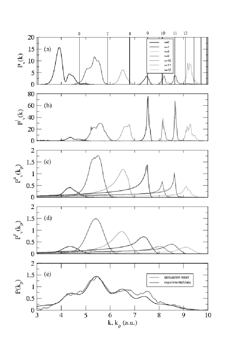
Figure 5: Successive steps for a theory-versus-experiment comparison of photodissociation spectrum for a laser energy 0.7 mJ (last row in the Table 1). Panel (a) gives the individual probabilities of initial vibrational levels $v$=6,…,12 in the molecular frame, for $\theta=0$, and as a function of $k$. Panel (b) takes into account the spatial intensity distribution of the laser. Panel (c) displays the intensity averaged probabilities after Abel transformation bringing them in the laboratory frame, for $\alpha=0$ and as a function of $k_{\rho}$. Panel (d), same as c but after convolution by the detector resolution window. Panel (e) sums up all individual v contributions and compares with the experimental spectrum.

Figure 5 panel (c) displays the dissociation probabilities $P^{a}_{v}(k_{\rho})$ as functions of $k_{\rho}$ after the Abel transformation Eq.(41). The basic difference with ${\cal P}^{i}_{v}(k)$ (panel b) is the rise of long range red tails of the individual peaks, especially for $v\geq 9$. This is due to the nonlinear features of the Abel transformation, mixing up a whole range of $\theta$-dependent probabilities for a single $\alpha$. Less aligned fragment distributions resulting from $v$=9,10,11 present tails that are much more marked than the ones coming from $v$=7 and 8.

The following step for building the experimental observable is the convolution with the detector resolution window which is taken as a square gate of 0.07 a.u. in kinetic momentum units, corresponding approximately to a pixel size of 70 $\mu m$. This as expected, results into the smoothing of very sharp structures such as the peaks associated with $v$=9 and 11 (pannel d).

Finally the theoretical spectrum is obtained as a sum of partial vibrational distributions with weights corresponding to the vibrational populations as given by Eqs(56-57). Panel (e) of figure 5 displays the resulting kinetic energy spectrum which is directly compared with the experimental one. An excellent agreement is obtained, the most noticeable differences occurring in the vicinity of $v$=9, which corresponds to an energy region particularly sensitive to possible inaccuracies related with the spatial intensity averaging of the laser.

The information we get from figure 5 can be summarized as follows: apart from the geometrical Abel transformation which is needed to bridge the dissociation probabilities evaluated in the ($k$-$\theta$) frame, to the photodissociation spectra as recorded on the detector plate, one has to take into consideration basically two additional facts, when attempting a quantitative interpretation of the experimental data:

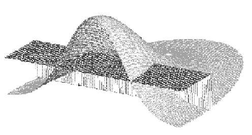
Figure 6: The laser field intensity distribution over the molecular beam.

i) The first is the spatial intensity distribution of the laser. Figure 6 displays a three-dimensional view of the relative spatial extensions of the laser focal area and that of the molecular beam as is actually the case in the experiments. Clearly, all the molecules are not subjected to the same intensity at a given time, requiring thus a spatial averaging, the role of which is one of the most striking.

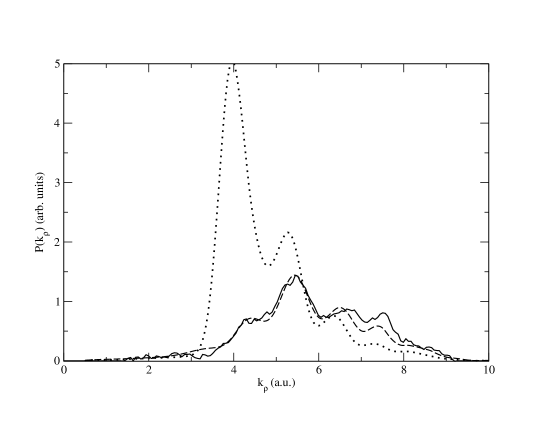
Figure 7: The dissociation probabilities calculated with (dashed line) and without (dotted line) averaging on the laser intensity distribution, versus experimental data (solid line).

Figure 7 gathers the spectra on the detector plate, for $\alpha=0$ and as a function of $k_{\rho}$ for two models: namely, with and without the spatial averaging over the laser intensity distribution. The results are compared to the experimentally recorded data. A huge decrease affects the spectrum in the momentum region extending from $k_{\rho}\simeq$ 3 to 5 a.u. when averaging over the field intensities. This precisely corresponds to the contributions of vibrational levels $v$=6,7 well protected against potential barriers that are high for lower intensities taking part in the averaging process. Thus the spatial averaging turns out to be crucial when comparing with experimental spectra.

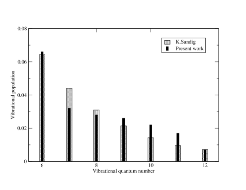
Figure 8: Vibrational levels populations as estimated by Sandig in 21 and fitted in the present work.

ii) The second is an accurate knowledge of the field-free vibrational populations of the parent ion H${}_{2}^{+}$, which take part in Eq.(56) through the function $a(v)$. Figure 8 displays in terms of histograms the relative vibrational populations of levels $v$=6,…,12 as they result from an estimation based on similar discharge experiments 21 . They are actually subjected to errors presumably within 10 to 15% in relative values.

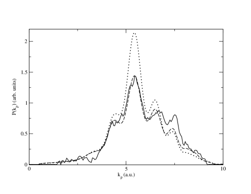
Figure 9: Dissociation probabilities calculated using Sandig 21 vibrational levels populations (dotted line) and the modified ones (dashed line) as compared with the experimental data (solid line).

A calculation based on them leads to the spectrum illustrated in figure 9 which basically disagrees with the experimental one over a region close to $k_{\rho}\simeq$ 5 to 6 a.u., corresponding to the most important peak. However, a nice agreement is obtained after some small modifications of the vibrational populations, not exceeding reasonable error bar limits and remaining within the overall decreasing behavior for high $v$’s, as is plotted in figure 8. It is worthwhile noting that this adjustment is done once for all, for given laser parameters (0.7 mJ of total energy) and is used hereafter for all other theory-versus-experiment comparisons.

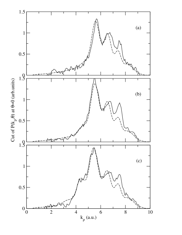
Figure 10: Cuts at $\alpha=0$ of the calculated (dashed line) and measured (solid line) kinetic momentum spectra for: (a) E₀=0.3 mJ; (b) E₀=0.5 mJ; (c) E₀=0.7 mJ.

The spectra are gathered within the frame of two one-dimensional representations: either as a function of the kinetic momentum $k_{\rho}$ or as a function of the angle $\alpha$ on the detector. Figure 10 gives the cuts (at $\alpha$=0) as a function of $k_{\rho}$, for three laser fields, whose characteristics are precisely the ones indicated on Table 1. It might be noted here that peak intensity value $I_{0}$ calculated using Eq.(62) strongly depends from the experimentaly measured parameters $b_{x}$, $b_{y}$ and $E_{0}$. In third column of Table 1 we give the intensities corresponding to the best agreement between experimental and calculated spectra presented on figure 10. This adjustment is necessary to reproduce correctly the left part of the spectra, which is particularly sensitive to the laser intensity, as can be seen in figure 7. We emphasized that this adjustment has only been performed for one-dimensional spectra corresponding to ($\alpha$=0). For the same pulse duration the laser intensities are ranging from low to medium and strong, following the panels a,b, and c. Three features can be emphasized:

i) Three major peaks are obtained, corresponding to the dissociation involving $v$=7, 8 and 9 levels, positioned in this order in the region $k_{\rho}\simeq$ 5 to 8 a.u. The theory-experiment agreement is good not only for the positions but also for the relative heights of these peaks; the most noticeable difference affecting again $v$=9, more sensitive to an accurate evaluation of the spatial intensity distribution;

ii) The strongest field (E₀=0.7 mJ, panel c) reveals the rise of an additional peak at the position of $v$=6. This is related with the bond softening mechanism, where the radiative coupling induces an important adiabatic barrier lowering, large enough for the population initially in the bound state $v$=6 to escape through tunneling. Excellent agreement with experimental results is obtained for this bump in the spectrum ;

iii) The blue tail of the spectrum extending above $k_{\rho}\simeq$ 8 a.u. corresponds to the photodissociation of initial populations on $v$=10,11 and 12, which due to possible vibrational trapping effects, is less efficient. Here again excellent theory-experiment agreement is reached.

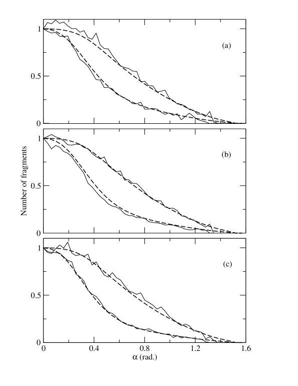
Figure 11: Angular distributions of photofragments for: (a) E₀=0.3 mJ; (b) E₀=0.5 mJ; (c) E₀=0.7 mJ. Solid lines correspond to experimental results, dashed lines to the calculated ones. (the upper pair to v=7 and the low one to v=8).

The angular distributions for the same field characteristics, are gathered in figure 11. They, precisely, correspond to $\alpha$-dependent 1D representations of fixed $k_{\rho}$-cuts of the 3D information of the type displayed in figure 3. This is done for two different values of $k_{\rho}$; namely $k_{\rho}$=5.5 a.u. and $k_{\rho}$=6.5 a.u. corresponding to the positions of the maximum amplitudes of the two major peaks of figure 10 attributed to $v$=7 and 8, respectively. The following observations can be pointed out:

i) These angular distributions, although labeled as $v$=7 and 8, actually contain informations originating from $v$=9,10,…, through the red-tail contributions of these levels (as is clear from figure 5 panel c). The excellent theory-versus-experiment agreement that is reached has to be judged within this intricate influence of the higher energy part of the spectrum. It is also worthwhile noting that due to larger experimental errors affecting $v$=9,10, angular distributions are not studied for higher $v$’s than 8.

ii) $v$=7 is much better aligned than $v$=8. This is basically due to the bond softening mechanism. A high potential barrier at $\theta=\pi/2$ protects $v$=7 population against photodissociation. This barrier is lowered at $\theta$=0 or $\pi$ where the radiative coupling is at its maximum, leading to efficient alignment, that is even better for increasing intensity. In other words the wavepacket associated with $v$=7 has to skirt around a high potential barrier at $\theta=\pi/2$ before dissociating, whereas the one associated with $v$=8 being closer to the top of the barrier can more easily tunnel. The consequence is that dissociation is facilitated for $\theta$=0, or $\pi$, when the initial population lies on $v$=7.

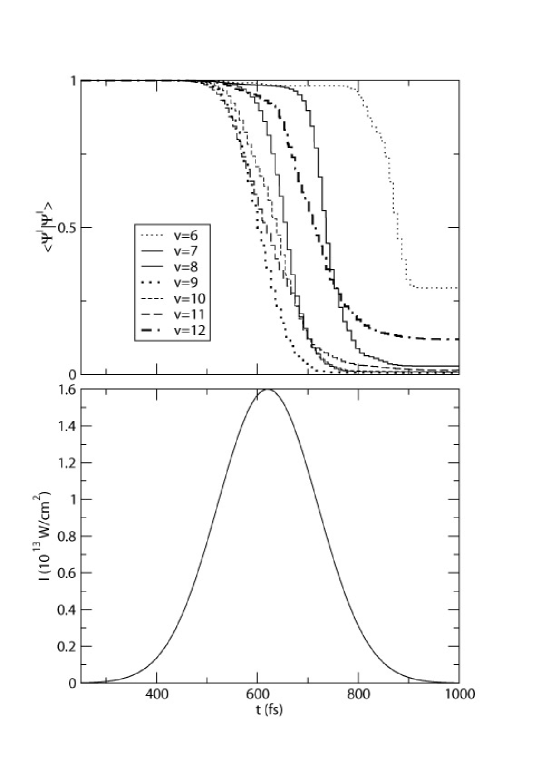
Figure 12: Time-resolved decay dynamics of individual vibrational levels in correspondance with the temporal laser intensity distribution.

A better understanding and interpretation of the way following which these complementary bound softening and vibrational trapping mechanisms ultimately affect the dissociation process, could be gained by a dynamical investigation. Figure 12 illustrates a time-resolved decay dynamics of individual vibrational levels. The lower panel gives the temporal shape of the laser intensity for the strongest field into consideration (E₀=0.7 mJ, with the parameters of the last row of Table 1). The decay dynamics is given in terms of the decrease of the short range population as a function of time, starting from a given $v$ of the parent ion H${}_{2}^{+}$ (i.e. the time dependence of the norm of the internal region wavepacket $||\Phi^{I}||^{2}$, as defined in subsection 2.1). The behavior of different $v$’s can be classified as follows:

$\bullet$ Levels affected by the bond softening mechanism; namely $v$=6,7,8. The decay starts only after the maximum of the laser pulse, which is required for the potential barriers to be sufficiently lowered. Although the decay mechanism is rather fast (the slope of $||\Phi^{I}||^{2}$ versus time is large), the photodissociation starting from $v$=6 is not complete, due to the fact that the potential barrier is closed before total escape towards the asymptotic region.

$\bullet$ $v$=9 which lies at the curve crossing region dissociates completely and faster than all other levels;

$\bullet$ Levels affected by the vibrational trapping mechanism; namely $v$=10,11,12. The populations of these levels start to dissociate during the laser rise time, but about the maximum intensity their decay rate is lowered (the slope of $||\Phi^{I}||^{2}$ versus time lower than the one of levels $v$=6,7,8). This is basically due to the fact that they are vibrationaly trapped in the temporarily closed upper adiabatic potential. It is also interesting to note that the population of $v$=12, trapped during the radiative interaction, partially returns back to the ground state bound potential, in such a way that dissociation starting from $v$=12 is not complete.

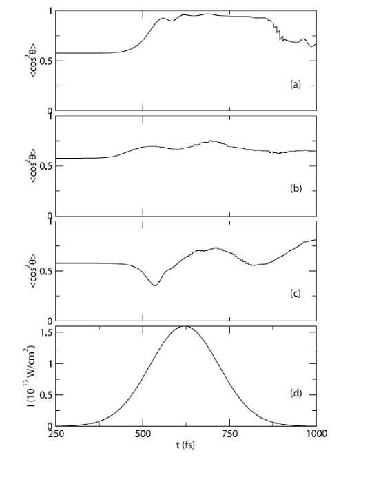
Figure 13: Average values of $<\cos^{2}\theta>$ for the different vibrational levels: (a) v=6; (b) v=9; (c) v=12 ;(d) - laser temporal profile.

The dynamical alignment characteristics are illustrated in figure 13. Here again the lower panel indicates the temporal shape of the strongest laser. The upper panels display the average value of $\langle\cos^{2}\theta\rangle$ on the internal region wavepacket; i.e. $\langle\Phi^{I}|\cos^{2}\theta|\Phi^{I}\rangle/\langle\Phi^{I}|\Phi^{I}\rangle$, indicating the alignment characteristics of the parent ion H${}_{2}^{+}$ as a function of time. Three initial levels are in consideration, each pertaining to one of the previously selected classes. The bond softening mechanism leading to the dissociation of $v$=6 (panel a) results into very efficient alignment during the pulse, which even remains during the fall off regime.

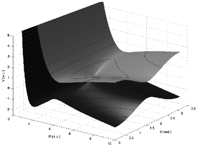
Figure 14: 3D adiabatic representation of the H${}_{2}^{+}$ potential energy surfaces in the presence of the field with peak intensity $I_{0}=7.5\times 10^{12}$ W/cm².

A thorough interpretation, already given in the literature 24 , can be summarized by referring to a three dimensional representation of the adiabatic potential energy surfaces (displayed in figure 4). This is provided in figure 14 for a single photon dressed ground and excited states of H${}_{2}^{+}$ including (by diagonalization) the radiative interaction. The photodissociation dynamics starting from $v$=6 is described by a wavepacket that evolves on the lower adiabatic potential surface. It has first to skirt around the potential barrier at $\theta=\pi/2$ and end up in the lower energy valley at $\theta=0$ or $\pi$. This is why fragments originating from a parent ion in an initial state well protected by a hardly penetrable potential barrier (as for $v$=6,7,8) are well aligned through the bond softening mechanism. On the opposite situation are parent ions in an initial state basically pertaining to the upper adiabatic potential energy surface (as for $v$=10,11,12). This surface presents a minimum around $\theta=\pi/2$, where the population is temporarily trapped. The dissociation by a single photon absorption further proceeds by a non-adiabatic transition to the lower adiabatic surface. Such a transition is more efficient for $\theta\simeq\pi/2$ (induced by a lower radiative coupling). Although the last step which is the evolution on the lower adiabatic surface tends to align the fragments, this effect is less efficient as the parent ion is prepared at $\theta\simeq\pi/2$ on this surface. The result is clearly understandable in terms of this vibrational trapping mechanism for $v$=12 (panel c, figure 13). During the rise time of the laser pulse, the parent ion is well trapped on the upper adiabatic surface leading to a misalignment (the bump of the $\langle\cos^{2}\theta\rangle$ curve at about $t$=550 fs). There is no noticeable alignment during the whole duration of the pulse. A second misalignment, probably due to the nonadiabatic jump, is obtained at $t$=800 fs. Finally $v$=9 which is basically not affected neither by bond softening, nor by vibrational trapping, does not show any alignment characteristics as is clear from panel b.

IV Conclusion

Once the competition between multiphoton ionization and dissociation processes is discarded by preparing the parent ion H${}_{2}^{+}$ through an electric discharge experiment, a rather simple and complete quantum modelisation is provided for a theory-versus-experiment comparison of angularly resolved kinetic energy spectra of photofragments resulting from intense field dissociation. An Abel transformation relates the probability ${\cal P}(k,\theta)$ for a single H${}_{2}^{+}$ molecule in a given initial ro-vibrational state, to dissociated with kinetic momentum $k$ along its polar direction $\theta$ with respect to the laser polarization vector, to $P(k_{\rho},\alpha)$, the probability for the photofragment H to be detected on a pixel of the detector plate labeled by its polar coordinates ($\rho,\alpha$), A quantitative reproduction of experimental data requires some statistics over initial ro-vibrational states on one hand and over the spatial distribution of laser intensities interacting with molecules positioned at different places in the ionic beam, on the other hand.

An excellent agreement is obtained with experimental spectra and especially for the alignment characteristics of the photofragments. A thorough interpretation can be conducted for single vibrational peaks of the spectra in terms of basic mechanisms, such as bond softening and vibrational trapping. The most striking observation is the major role the laser volume effect is playing, in particular over lower vibrational levels.

Among our feature prospects, is the elucidation of the role of isotope effects in the photodissociation of D${}_{2}^{+}$ and HD⁺, which are currently studied in H.Figger’s group.

Appendix

This appendix is devoted to some geometrical and and vector relations illustrated in figure 2. $\boldsymbol{r_{1}}$ and $\boldsymbol{r_{2}}$ are the vectors pointing H and H⁺ in the laboratory frame, $\boldsymbol{R}$ and $\boldsymbol{R_{G}}$ defined by

$$\boldsymbol{R}=\boldsymbol{r_{1}}-\boldsymbol{r_{2}}$$ (A-1)

$$\boldsymbol{R_{G}}=vt\boldsymbol{u_{y}}=\frac{1}{2}(\boldsymbol{r_{1}}+\boldsymbol{r_{2}})$$ (A-2)

are the relative internuclear separation and the position of the center of mass $G$, respectively (by neglecting the contribution of the electron). The right-angle triangles $OO^{\prime}M$ and $O^{\prime}M^{\prime}M$ lead to:

$$\left|\left|\frac{1}{2}\boldsymbol{R}\right|\right|^{2}=\rho^{2}+(D-vt)^{2}$$ (A-3)

and

$$||\boldsymbol{r}||^{2}=\rho^{2}+D^{2}$$ (A-4)

whereas from the triangle $MGO$ one gets:

$$\frac{1}{2}\boldsymbol{R}=\boldsymbol{r}-\boldsymbol{R_{G}}.$$ (A-5)

The unitary vector $\boldsymbol{u_{R}}$ along $\boldsymbol{R}$, can be easily evaluated using Eqs(A-2,A-3) and Eq.(A-5):

$$\boldsymbol{u_{R}}=\frac{\boldsymbol{R}}{\left|\left|\boldsymbol{R}\right|\right|}=\frac{\boldsymbol{r}-vt\boldsymbol{u_{y}}}{\left[\rho^{2}+(D-vt)^{2}\right]^{1/2}}$$ (A-6)

and its projection over $\boldsymbol{u_{y}}$ is nothing but:

$$\boldsymbol{u_{R}}\cdot\boldsymbol{u_{y}}=\frac{\boldsymbol{r}\boldsymbol{u_{y}}-vt||\boldsymbol{u_{y}}||^{2}}{\left[\rho^{2}+(D-vt)^{2}\right]^{1/2}}=\frac{D-vt}{\left[\rho^{2}+(D-vt)^{2}\right]^{1/2}}$$ (A-7)

taking into account: $\boldsymbol{r}\cdot\boldsymbol{u_{y}}=D$.

The polar angles $\theta$ and $\alpha$ positionning H (and $M$) in the center of mass and detector frames can be related using the right-angle triangle $GM^{\prime}M$:

$$\cos\theta=\frac{HH^{\prime}}{||\frac{1}{2}\boldsymbol{R}||}=\frac{\rho\cos\alpha}{||\frac{1}{2}\boldsymbol{R}||}$$ (A-8)

or finally taking into account Eq.(A-3):

$$\cos\theta=\frac{\rho\cos\alpha}{\left[\rho^{2}+(D-vt)^{2}\right]^{1/2}}.$$ (A-9)

References

- (1) :
- (2) P.H. Bucksbaum A. Zavriev, H.G. Muller, and D.W. Schumacher, Phys.Rev.Lett, 64, 1883 (1990);
- (3) A. Zavriev, P.H. Bucksbaum, H.G. Muller, and D.W. Schumacher, Phys.Rev.A, 42, 5500 (1990);
- (4) J.D. Buck, D.H. Parker, and D.W. Chandler, J.Phys.Chem, 92, 3701 (1988);
- (5) L.J. Frasinski, J.H. Posthumus, J. Plumridge, K. Codling, P.F. Taday and A.J. Langley, Phys.Rev.Lett, 83, 3625, (1999);
- (6) T.D.G. Walsh, F.A. Ilkov, S. L. Chin, F. Châteauneuf, T.T. Nguyen-Dang, S. Chelkowski, A.D. Bandrauk and O. Atabek, Phys. Rev. A, 58, 3922, (1998);
- (7) D.W. Chandler,D.W.Neyer, A.J.Heck, Proc.SPIE, 3271, 104 (1998); F. Rosca-Pruna, E. Springate, H.L. Offerhaus, M. Krishnamurthy, N. Farid, C. Nicole and M.J.J. Vrakking, J. Phys.B, 34, 4919 (2001);
- (8) A.Giusti-Suzor, X.He, O.Atabek, and F.H.Mies Phys.Rev.Lett, 64, 515 (1990); E.E. Aubanel, A. Conjusteau, A.D. Bandrauk, Phys.Rev.A. 48, R4011 (1993); E.E. Aubanel, A. Conjusteau, A.D. Bandrauk,E.E. Aubanel,J.M. Gauthier Molecules in Laser Fields (Marcel Dekker Inc., New-York, 1994)
- (9) P.Dietrich and P.B.Corkum, J. Chem. Phys., 97, 3187 (1992); A. Conjusteau and A.D. Bandrauk, J. Chem. Phys., 106, 9095 (1997);
- (10) A. Giusti-Suzor, F.H. Mies, L.F. Dimauro, E. Charron and B. Yang J.Phys.B, 28, 309 (1995)
- (11) F. Châteauneuf, T.T Nguyen Dang, N. Ovellet and O.Atabek, J. Chem. Phys., 108, 3974 (1998); H. Abou-Rachid, T.T. Nguyen-Dang and O. Atabek, J. Chem. Phys., 110, 4737 (1998); ibid, 114, 2197 (2001)
- (12) O. Atabek, M. Chrysos, and R. Lefebvre, Phys. Rev. A, 49, R8, (1994); O. Atabek, T.T. Nguyen-Dang J.Mol.Structure (Theochem), 493, 89, (1999);
- (13) A. Kondorskiy and H. Nakamura, Phys. Rev. A, 66, 053412, (2002);
- (14) K .Sändig, H. Figger, and T.W. Hänsch, Phys.Rev.Lett, 85, 4876 (2000); K. Sändig, H. Figger, Ch. Wunderlich, and T. W. H nsch, Proceedings of the XIV International Conference on Laser Spectrosopy, Innsbruck, 1999 (World Scientific, Singapore, 1999), p. 310; K. Sändig, H. Figger, and T. W. H nsch, Multiphoton Processes, Proceedings of the ICOMP VIII (8th International Conference), Monterey, California 1999, Ed. L.F. DiMauro, R.F. Freeman, K.C. Kulander, AIP Conference Proceedings, 525 (2000). 1999 (World Scientific, Singapore, 1999), p. 310;
- (15) J.M.Combes, R.G. Newton and R. Shtokhamer, Phys.Rev.D, 11, 366 (1975);
- (16) J.D.Dollard, Comm.Math.Phys, 12, 193 (1969);
- (17) I.D. Williams, P. McKenna, B. Srigengan, I.M.G. Johnston, W.A. Bryan, J.H. Sanderson, A. El-Zein, T.R.J. Goodworth, W.R. Newell, P.F. Taday and A.J.Langley, J. Phys.B, 33, 2743 (2000);
- (18) R. Numico, A. Keller, and O. Atabek, Phys.Rev.A, 52, 1298 (1995);
- (19) R. Numico, A. Keller, and O. Atabek, Phys.Rev.A, 57, 2841 (1998);
- (20) A. Carrington, R.A. Kennedy, in Gas Phase Ion Chemistry, ed M.T. Bowers, 3, 393, (1984);
- (21) B.R. Judd, Angular momentum theory for diatomic molecules, Academic Press, (1975);
- (22) W.H. Press, B.R. Flannery, S.A. Teukolsky, W.T. Vetterling, in Numerical Recipes, Cambridge Universtiy Press, (1986);
- (23) C.E. Dateo and H. Metiu, J. Chem. Phys., 95, 7392 (1991);
- (24) A. Keller, Phys.Rev.A, 52, 1450 (1995);
- (25) M.D. Feit, J.A. Fleck, and A. Steiger, J. Comp. Phys., 47, 412 (1982); R.Kosloff, J. Phys. Chem., 92, 2087 (1988);
- (26) H. Figger, D. Pavicic, Private communications (2002);
- (27) K. Sändig, PhD thesis, Max Planck Institute of Quantum Optics (2000);
- (28) M. Daumer, D. Dürr, S. Goldstein, N. Zanghi, Journal of Statistical Physics 88, 967-977 (1997);
- (29) R. Bracewell, The Fourier Transform and Its Applications, 3rd ed. New York: McGraw-Hill, (1999);
- (30) B.J. Whitaker, Photo-ion imaging techniques and reactive scattering, Research in Chemical Kinetics, Vol 1., eds. RG Compton and G Hancock. Elsevier 1993, pp 307-346; R.N. Strickland and D.W. Chandler, Appl. Optics., 30 (1991) 1811; Young-Jae Jung, Moon Soo Park, Yong Shin Kima, Kyung-Hoon Jungb and Hans-Robert Volpp, J. Chem. Phys., 111, 4005 (1999);
- (31) R. Numico, A. Keller, and O. Atabek, Phys.Rev.A, 60, 406 (1999);