Bohmian arrival time without trajectories

Abstract

The computation of detection probabilities and arrival time distributions within Bohmian mechanics in general needs the explicit knowledge of a relevant sample of trajectories. Here it is shown how for one-dimensional systems and rigid inertial detectors these quantities can be computed without calculating any trajectories. An expression in terms of the wave function $\Psi$ and its spatial derivative $\partial_{x}\Psi$, both restricted to the boundary of the detector’s spacetime volume, is derived for the general case, where the probability current at the detector’s boundary may vary its sign.

1 Introduction

A microscopic object $s$ may trigger a sudden change in the properties of a macroscopic system $S$. Often such events take place during an interval of time much shorter than the duration of the interaction between $s$ and $S$. Perhaps the simplest example is the detection time of a quantum particle which slowly passes a detector. This phenomenologically well accessible quantity is usually termed arrival time. Quantum theory has difficulties in identifying events and a fortiori their time of occurrence within its formalism, because, according to Schrödinger’s equation, the unitary state evolution of the closed system containing $s\$and $S$ does not make any sudden jumps. Jumps of states are introduced into the standard quantum formalism only through state reduction, which is supposed to happen in an open system, when a “measurement” is performed on it from “outside”. Yet in this case the instant of time of the reduction is not stochastic but rather determined by the observer’s deliberate choice. Thus state reduction does not seem to be the proper notion to understand the stochastic distribution of the time of events.

Attempts to obtain the arrival time distribution through the model of continuous observation leads to the well known quantum zeno paradox [1]. Also the proposals for a time operator (see e.g. [2]) are still subject to discussion and controversy [3, 4].

One strategy to incorporate detection events into quantum theory is by means of Bohmian mechanics (BM), which introduces the additional notion of particle trajectories into the standard formalism. Within this framework Leavens [5] and McKinnon and Leavens [6] derived an expression for the time resolved detection probability for one-dimensional (1D) scattering situations. Let $\Psi$ be a normalized solution of a time dependent 1D Schrödinger equation and $j$ its associated probability current density. In [5, 6] it has been argued for a Bohmian particle with wave function $\Psi$ that the detection probability at position $a$ between time $0$ and time $T>0$ is given by $\int_{0}^{T}\left|j(t,a)\right|dt$ . The line of argument assumes from the outset that no trajectory passes through $a$ more than once during the time interval $\left[0,T\right]$ which is guaranteed if $j(\cdot,a)$ does not change sign. (For an ideal detector the first entry triggers an event, e.g. by discharging the device and producing a click. Further on the detector is insensitive to additional entries.)

If, however, multiple crossings do occur, the replacement of $j(t,a)$ by a cut off current has been advocated by Daumer et al [8], such that only the first traversal of the trajectories should be counted. This means that the time intervals with second, third, etc. crossings should be dropped from the integral $\int_{0}^{T}\left|j(t,a)\right|dt$. Therefore the computation of such detection probabilities in general demands the explicit knowledge of the Bohmian trajectories of the problem at hand. Yet Bohmian trajectories are the solutions of a nonlinear system of ordinary differential equations and therefore difficult to obtain.

The general Bohmian notion of detection probability associated with quite arbitrary space-time regions has been formalized in [9]. As in the earlier treatment [8] Bohmian trajectories enter the formula defining the detection probability. Here we show how for 1D systems and rigid inertial detectors the Bohmian detection probability and the associated arrival time distribution can be computed under quite general circumstances without any knowledge of the Bohmian trajectories. The relevant formula is contained in proposition 4.

In section 2 we give a very short overview of the main ingredients of Bohmian mechanics, omitting mathematical detail. Section 3 introduces the essential mathematical structures needed for the formulation of one-dimensional arrival time problems in the framework of non-relativistic Bohmian mechanics. In section 4 then a reformulation of the arrival time distribution for one-dimensional detectors occupying spatial intervals $[a,b]$, with the mere aid of probability and current density integrals, is given and proved. Finally section 5 demonstrates the practical use of the technique given in section 4 by means of several numerical examples. Free evolution as well as evolution under the influence of external potentials is considered.

2 Bohmian Mechanics

BM rests on the insight that with each normalized solution of the time dependent Schrödinger equation, a fibration of the configuration space-time is given. At time $t$ each fibre (Bohmian trajectory) has a unique representative in the underlying configuration space, and therefore a dynamical evolution of configurations along the fibres follows. The local conservation of configuration space probability implies that its quantum mechanical evolution coincides with the one implied by the transport along the fibres. Therefore a causal deterministic interpretation of quantum mechanics in terms of movement in configuration space becomes consistent. An individual quantum system with wave function $\Psi$ within BM is now assumed to realize one of the system’s trajectories, i.e. at each instant the system is in a point of the configuration space. Amending the continuum notions of quantum theory by such point structures opens up the possibility to identify unique properties and sudden events within the formalism. Consequently one may ask again “Does a trajectory enter a certain spacetime region?” or “When is it, that the system’s trajectory enters a certain spacetime region?”.

Since the choice among the trajectories is beyond control, only probabilistic predictions can be made, yet at any time a system has properties without the need to invoke state reduction. Whenever the probabilistic predictions of BM can be compared with those of standard quantum mechanics, they agree. To us the prime achievement of BM seems to be, that it resolves the quantum measurement problem. A concise summary of Bohmian mechanics can be found in [10].

3 Arrival time from Bohmian flow

For the sake of simplicity, the set of Galilean spacetime points is assumed to be $\mathcal{M}=\mathbb{R}^{2}$. As a positively oriented, global and inertial chart we choose $id_{\mathcal{M}}=:(t,x)$. The associated tangent frame is denoted by $(\partial_{t},\partial_{x})$.

3.1 Bohmian velocity vector field and Bohmian flow

Let the mapping $\Psi:\mathcal{M}\rightarrow\mathbb{C}$ be $\mathcal{C}^{2}$ and a solution to the Schrödinger equation

$$\textrm{i}\hbar\partial_{t}\Psi=\left[-\frac{\hbar^{2}}{2m}\partial_{x}^{2}+V(x)\right]\Psi$$

with $V$ any real scalar potential. Then with the aid of the position and current densities

$$\rho:=\Psi^{*}\Psi$$

and

$$j:=\frac{\hbar}{m}\Im\left\{\Psi^{*}\left(\partial_{x}\Psi\right)\right\}$$

the current vector field $\hat{j}$ is defined as

$$\hat{j}:=\rho\partial_{t}+j\partial_{x}$$

on $\mathcal{M}$. If $\rho\neq 0,\;\forall p\in\mathcal{M}$ the corresponding Bohmian velocity vector field

$$v:=\partial_{t}+\frac{j}{\rho}\partial_{x}$$

is $\mathcal{C}^{1}$. The maximal integral curve of the vector field $v$ through a point $p\in\mathcal{M}$ is the unique function $\gamma:I_{p}\rightarrow\mathcal{M}$ with $\gamma(0)=p$ and

$$\dot{\gamma}(s)=v(\gamma(s)),\quad\forall s\in I_{p}$$

where $I_{p}$ is a non-extendable open real interval. Those integral curves are regarded to represent the worldlines of the actual Bohmian particles. We assume that $v$ is complete, which means that $I_{p}=\mathbb{R}$, for all $p\in\mathcal{M}$. Then the mapping

$$F:\mathbb{R}\times\mathcal{M}\rightarrow\mathcal{M},\;(s,p)\mapsto\gamma_{p}(s)$$

is a global flow on $\mathcal{M}$ with $F(r,F(s,p))=F(r+s,p)$. As $t\circ F(s,p)=t\circ\gamma_{p}(s)=s+t(p)$, no worldline begins or ends at a finite time. Moreover $F(s,\cdot)$ bijectively maps instantaneous spaces $\Sigma_{\tau}=\{p\in\mathcal{M}/\;t(p)=\tau\}$ onto instantaneous spaces, namely $F(s,\Sigma_{r})=\Sigma_{s+r}$.

3.2 Conservation of probability

By inserting $\hat{j}$ as the first argument into the volume form $E=dt\wedge dx$, we get the current-1-form

$$J:=\hat{j}\lrcorner E=\rho\textrm{d}x-j\textrm{d}t.$$

Due to the continuity equation $\partial_{t}\rho+\partial_{x}j=0$ the current form $J$ is closed:

$$\textrm{d}J=(\partial_{t}\rho+\partial_{x}j)\textrm{d}t\wedge\textrm{d}x=0.$$

For any spacetime region $D$ with piecewise $\mathcal{C}^{1}$-boundary $\partial D$, Stoke’s theorem therefore assures that

$$\int_{\partial D}J=\int_{D}\textrm{d}J=0.$$ (1)

In particular for spacetime regions of the form indicated in figure 1, equation (1) for any Borel set $X$ results in

$$\int_{X}J=\int_{F(s,X)}J.$$ (2)

Fig. 1: Spacetime region $D$ enclosed by integral curves and instantaneous sets

Equation (2) can be seen as follows: Let $\partial D$ be oriented “anticlockwise” (direction of integration), then

$$\int_{\partial D}J = \int_{X}J+\underbrace{\int_{\gamma_{p_{1}}([r,r+s])}J}_{(a)}-\int_{F(s,X)}J-\underbrace{\int_{\gamma_{p_{2}}([r,r+s])}}_{(b)}J.$$

Since

$$\int_{\gamma_{p}([\alpha,\beta])}J = \int_{\alpha}^{\beta}J(\dot{\gamma}_{p}(s))\textrm{d}s=\int_{\alpha}^{\beta}J(v_{\gamma_{p}(s)})\textrm{d}s$$

$$= \int_{\alpha}^{\beta}v\lrcorner(\hat{j}\lrcorner E)_{\gamma_{p}(s)}\textrm{d}s=\int_{\alpha}^{\beta}\frac{1}{\rho}E(\hat{j},\hat{j})_{\gamma_{p}(s)}\textrm{d}s=0$$

the contributions $(a)$ and $(b)$ to $\int_{\partial D}J$ vanish: $(a)=(b)=0$.

For an interval $X\subseteq\Sigma_{\tau}$ integrals of the form (2) expressed in our chosen coordinates read as

$$\int_{X}J=\int_{X}(\rho\textrm{d}x-j\textrm{d}t)=\int_{\min(x(X))}^{\max(x(X))}\rho(\tau,\xi)\textrm{d}\xi$$ (3)

which is easily recognized as the standard quantum mechanical probability for “finding a particle” at time $\tau$ in the spatial interval $[\min(x(X)),\max(x(X))]$, as soon as $\rho$ is integrable and normalized, i.e. $\int_{-\infty}^{\infty}\rho(\tau,\xi)\textrm{d}\xi=\int_{-\infty}^{\infty}\Psi^{*}\Psi(\tau,\xi)\textrm{d}\xi=1$, which will further on be assumed to hold. Equation (2) can then be interpreted as the conservation of probability along the flow lines of the Bohmian vector field. In other words, the amount of probability contained in $X$ is the same as in $F(s,X)$, for all $s\in\mathbb{R}$. Note that for a complete vector field $v$, we get a fibration of $\mathcal{M}$ into the images of the integral curves or orbits of $v$. Equation (3) then induces a measure on the space of these orbits, independently of the choice of $\tau$, which will be argued below.

Having this in mind, the amount of probability contained in the set of Bohmian orbits passing through quite arbitrary spacetime regions $D$, which need not be subsets of an instantaneous space, can be defined in a straightforward and unambiguous manner: We simply take the probability (3) of the intersection of all the flow lines, passing through $D$, with an arbitrary hypersurface $\Sigma_{\tau}$.

Let $\pi$ be the projection $\pi:\mathbb{R}\times\mathcal{M}\rightarrow\mathcal{M},\;(s,p)\mapsto p$ and let $F_{\tau}$ be the restriction of $F$ onto $\mathbb{R}\times\Sigma_{\tau}$. Then the mapping

$$\mathcal{F}_{\tau}:=\pi\circ F_{\tau}^{-1}:\mathcal{M}\mapsto\Sigma_{\tau}$$

is the fibre projection of $\mathcal{M}$ onto the instantaneous subspace $\Sigma_{\tau}$ along the Bohmian trajectories. If $\mathcal{F}_{\tau}(D)$ is a Borel set in $\Sigma_{\tau}$ then we define the transition of the Bohmian vector field through $D$ as

$$T(D)=\int_{\mathcal{F}_{\tau}(D)}J.$$

With $\mathcal{X}_{\tau}:=x\circ\mathcal{F}_{\tau}$ delivering the $x$-coordinates of the fibre projection $\mathcal{F}_{\tau}$ this yields

$$T(D)=\int_{\mathcal{X}_{\tau}(D)}\rho(\tau,\xi)\textrm{d}\xi.$$

Relation (2) secures that $T(D)$ is independent of the choice of the instantaneous subspace $\Sigma_{\tau}$, or respectively of the choice of $\tau$. In what follows we will restrict ourselves to $\mathcal{F}_{0}$ and $\mathcal{X}_{0}$ respectively.

Remark 1

$T$ does not induce a measure on the Borel subsets of $\mathcal{M}$, as $T(D_{1}\cup D_{2})\neq T(D_{1})+T(D_{2})$ in general, for $D_{1}\cap D_{2}=\emptyset$. For regions $D_{1}\subseteq D_{2}$ it is however guaranteed, that $\mathcal{F}_{0}(D_{1})\subseteq\mathcal{F}_{0}(D_{2})$, and therefore $\mathcal{X}_{0}(D_{1})\subseteq\mathcal{X}_{0}(D_{2})$, as all the trajectories passing through $D_{1}$ obviously also contribute to the transition through $D_{2}$. I.e. for $D_{1}\subseteq D_{2}$ the relation $T(D_{1})\leq T(D_{2})$ holds.

3.3 Arrival time distribution

Having the notion of transition through a spacetime region $D$, the definition of detection probabilities is obtained easily. For a spacetime region $D\subseteq\mathcal{M}$ we define the subsets

$$D_{\tau}:=\{p\in D/\;t(p)\leq\tau\}$$ (4)

as indicated in figure 2. The transition $T(D_{\tau})$ of flow lines through $D_{\tau}$ then is the probability for a Bohmian particle, to have “arrived” in the region $D$ before time $\tau$. If $D$ is furthermore assumed to be the spacetime region occupied by a 100% efficient, purely passive detecting device, which “clicks” as soon as a particle, i.e. it’s Bohmian trajectory, enters it, then the transition $T(D_{\tau})$ finds it’s interpretation as detection probability up to time $\tau$.

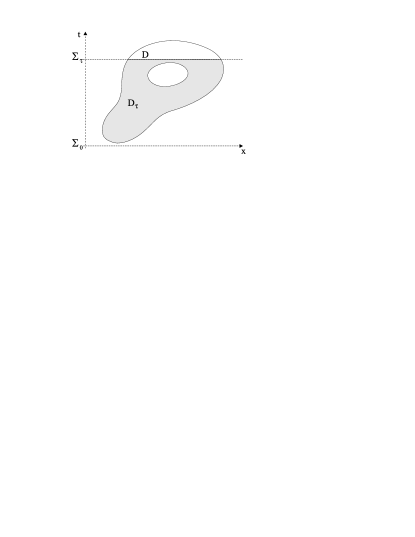
Fig. 2: Subsets $D_{\tau}$ of a spacetime region $D$

Definition 2

For a spacetime region $D$ with subsets $D_{\tau}$ (4), whose fibre projections $\mathcal{F}_{0}(D_{\tau})$ are Borel sets for every $\tau\in\mathbb{R}$, the detection probability

$$P_{D}(\tau):=T(D_{\tau})=\int\limits_{\mathcal{F}_{0}(D_{\tau})}J=\int\limits_{\mathcal{X}_{0}(D_{\tau})}\rho(0,\xi)\textrm{d}\xi$$

is, as a function of time $\tau\in\mathbb{R}$, positive, monotonically increasing and bounded.

The positivity is guaranteed because of the positivity of the probability density $\rho=\Psi^{*}\Psi$, the monotonicity because of $D_{\tau_{1}}\subseteq D_{\tau_{2}}$ for $\tau_{1}\leq\tau_{2}$ and remark 1. $P$ is bounded because the transition $T(D)$ is bounded by 1 for any spacetime region $D$.

Interpretatively the quantity $N:=\lim\limits_{\tau\to\infty}P_{D}(\tau)$ represents the overall probability for a detection event in $D$. Now taking only that part of Bohmian world lines into account, which enter the spacetime region $D$ at some time, and therefore produce a detection event, $\frac{1}{N}P_{D}(\tau)$ delivers the conditional probability for a detection event up to time $\tau$.

Definition 3

Let $P_{D}$ be the detection probability function of definition 2, then by the function

$$P_{D}^{c}:=\frac{P_{D}}{\lim\limits_{\tau\to\infty}P_{D}(\tau)}:\mathbb{R}\rightarrow[0,1]$$

the conditional arrival time distribution for a spacetime region $D$ shall be denoted.

The lower index of $P_{D}$ and $P_{D}^{c}$ respectively will further on be omitted, if it is evident from the context, which spacetime region $D$ is meant.

4 Formulation without trajectories

From now on we consider detectors occupying spacetime regions of the form

$$D=\{p\in\mathcal{M}/x(p)\in[a,\,b],\;t(p)\geq 0\}$$ (5)

which corresponds to a detector being at rest with respect to our inertial chart, occupying the interval $[a,\,b]$, and being sensitive from time $t=0$ onward. For $b\to a$ we get the point detector at $x=a$.

Again we have the subsets

$$D_{\tau}=\{p\in D/\;t(p)\leq\tau\}.$$

Proposition 4

For the detection probability function $P$ for a spacetime region of type (5) the formula

$$P(\tau)=P(0)+\max\{f_{a}(s)/\;0\leq s\leq\tau\}+\max\{-f_{b}(s)/\;0\leq s\leq\tau\}$$ (6)

holds for times $\tau\geq 0$, with

$$f_{a}(s)=\int_{0}^{s}j(t,a)\textrm{d}t\qquad\textrm{and}\qquad f_{b}(s)=\int_{0}^{s}j(t,b)\textrm{d}t$$

being antiderivatives of the current densities at $x=a$ and $x=b$, respectively.

Proof: From remark 1 we know that

$$P(\tau)=T(D_{\tau})=\int\limits_{\min(\mathcal{X}_{0}(D_{\tau}))}^{\max(\mathcal{X}_{0}(D_{\tau}))}\rho(0,\xi)\textrm{d}\xi\;\geq\;P(0)=T(D_{0})=\int\limits_{a}^{b}\rho(0,\xi)\textrm{d}\xi$$

and also that

$$\min(\mathcal{X}_{0}(D_{\tau}))\leq a\qquad\textrm{and}\qquad\max(\mathcal{X}_{0}(D_{\tau}))\geq b$$

as $\mathcal{X}_{0}(D_{0})=[a,\,b]\subseteq\mathcal{X}_{0}(D_{\tau})$, which allows the separation

$$P(\tau) = \int\limits_{\min(\mathcal{X}_{0}(D_{\tau}))}^{a}\rho(0,\xi)\textrm{d}\xi+\int\limits_{a}^{b}\rho(0,\xi)\textrm{d}\xi+\int\limits_{b}^{\max(\mathcal{X}_{0}(D_{\tau}))}\rho(0,\xi)\textrm{d}\xi$$ (7)

$$= \int\limits_{\min(\mathcal{X}_{0}(D_{\tau}))}^{a}\rho(0,\xi)\textrm{d}\xi+P(0)+\int\limits_{b}^{\max(\mathcal{X}_{0}(D_{\tau}))}\rho(0,\xi)\textrm{d}\xi.$$

The non-crossing property of Bohmian trajectories secures that

$$\mathcal{X}_{0}(\{(t,a)\})\leq\mathcal{X}_{0}(\{(t,x)\}),\quad\forall\;x\geq a$$

and

$$\mathcal{X}_{0}(\{(t,x)\})\leq\mathcal{X}_{0}(\{(t,b)\}),\quad\forall\;x\leq b.$$

This allows the reformulation of (7) into

$$P(\tau) = P(0)$$ (8)

$$+ \int_{\min(\mathcal{X}_{0}(D_{\tau}^{a}))}^{a}\rho(0,\xi)\textrm{d}\xi$$

$$+ \int_{b}^{\max(\mathcal{X}_{0}(D_{\tau}^{b}))}\rho(0,\xi)\textrm{d}\xi$$ (9)

with

$$D_{\tau}^{a}=\{p\in D_{\tau}/\;x(p)=a\}$$

and

$$D_{\tau}^{b}=\{p\in D_{\tau}/\;x(p)=b\}$$

being the restrictions to the right, respectively left, edges of $D_{\tau}$. Because of the positivity of the position density $\rho$, by applying Stoke’s theorem to regions as illustrated in figure 3, term (8) can be expressed as

$$\int_{\min(\mathcal{X}_{0}(D_{\tau}^{a}))}^{a}\rho(0,\xi)\textrm{d}\xi = \max\limits_{0\leq t\leq\tau}\left\{\int_{\mathcal{X}_{0}(\{(t,a)\})}^{a}\rho(0,\xi)\textrm{d}\xi\right\}$$

$$=\max\limits_{0\leq t\leq\tau}\left\{\int_{0}^{t}j(s,a)\textrm{d}s\right\} = \max\left\{f_{a}(t)/\;0\leq t\leq\tau\right\}.$$ (10)

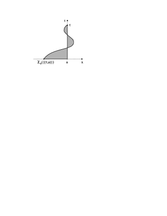
Fig. 3: Spacetime region

Analogously term (9) becomes

$$\int_{b}^{\max(\mathcal{X}_{0}(D_{\tau}^{b}))}\rho(0,\xi)\textrm{d}\xi = \max\limits_{0\leq t\leq\tau}\left\{\int_{b}^{\mathcal{X}_{0}(\{(t,b)\})}\rho(0,\xi)\textrm{d}\xi\right\}$$

$$=\max\limits_{0\leq t\leq\tau}\left\{\int_{t}^{0}j(s,b)\textrm{d}s\right\} = \max\left\{-f_{b}(t)/\;0\leq t\leq\tau\right\}.$$ (11)

Equation (7) together with (10) and (11) finally reads

$$P(\tau)=P(0)+\max\{f_{a}(s)/\;0\leq s\leq\tau\}+\max\{-f_{b}(s)/\;0\leq s\leq\tau\}$$

which completes the proof.   

Taking the limit $b\to a$ we immediately get the detection probability for point detectors:

Corollary 5

For spacetime regions of the form

$$D=\{p\in\mathcal{M}/\;x(p)=a,\,t(p)\geq 0\}$$

the detection probability function $P$ can be expressed as

$$P(\tau)=\max\{f_{a}(s)/\;0\leq s\leq\tau\}+\max\{-f_{a}(s)/\;0\leq s\leq\tau\}$$

with

$$f_{a}(s)=\int_{0}^{s}j(t,a)\textrm{d}t$$

being an antiderivative of the current density at $x=a$.

The conditional arrival time distribution associated with the spacetime region (5)

$$P^{c}:=\frac{P}{\lim\limits_{s\to\infty}P(s)}:\mathbb{R}\rightarrow[0,1]$$

obeys $P^{c}(\tau)=0$ for $\tau<0$. $P^{c}(0)>0$ holds for $a<b$, since $\rho>0$. For $\tau>0$ $P^{c}$ is continuous and $P^{c}$ is non-decreasing. Thus $P^{c}$ is the distribution function of a Lebesgue-Stieltjes measure $\mu$ [11]. $\mu$ can be separated into a point measure $\mu_{s}$, which ascribes to every Borel set $A\subseteq\mathbb{R}$ the value $P^{c}(0)$ if $0\in A$, the value 0 otherwise, and an absolutely continuous part $\mu_{ac}$, with respect to the Lebesgue measure. That is, there exists a Lebesgue-measurable density function $\delta$ on $\mathbb{R}$, which vanishes for $\tau\leq 0$ and ascribes to every interval $[a,b]$ the value

$$\mu_{ac}([a,b])=P^{c}(b)-P^{c}(a)=\int_{a}^{b}\delta(s)\textrm{d}s$$

if $0<a<b$. $\mu$ finally reads as $\mu=\mu_{s}+\mu_{ac}$

The density $\delta$ is needed for the calculation of the expectation values and variances of the arrival time, represented by the stochastic variable

$$T^{A}:\mathbb{R}\to\mathbb{R},\tau\mapsto\tau.$$

If the relevant integrals exist, they can be obtained in the usual manner:

$$\langle T^{A}\rangle_{\mu}=\langle T^{A}\rangle_{\mu_{s}}+\langle T^{A}\rangle_{\mu_{ac}}=0\cdot P^{c}(0)+\int_{0}^{\infty}\tau\cdot\delta(\tau)\textrm{d}\tau=\int_{0}^{\infty}\tau\cdot\delta(\tau)\textrm{d}\tau$$

and

$$\mathcal{V}_{\mu}(T^{A})=\langle(T^{A})^{2}\rangle_{\mu}-\langle T^{A}\rangle_{\mu}^{2}.$$

Remark 6

The probability density $\delta$ on $]0,\infty[$ takes the form

$$\delta(\tau) = \left(\lim\limits_{t\rightarrow\infty}P(t)\right)^{-1}\cdot\left[j(\tau,a)\cdot\Theta\left(f_{a}(\tau)-\max\limits_{0\leq s\leq\tau}\{f_{a}(s)\}\right)\right.$$ (12)

$$- \left.j(\tau,b)\cdot\Theta\left(-f_{b}(\tau)-\max\limits_{0\leq s\leq\tau}\{-f_{b}(s)\}\right)\right]$$

where $\Theta$ denotes the step function $\Theta(s)=\left\{\begin{array}[]{cc}0&s<0\\ 1&s\geq 0\end{array}\right.$.

The formulation for a point detector at $x=a$ is simply achieved by replacing $b$ with $a$ everywhere in (12).

This shows, that it is not enough to know the current density at a given instant $\tau$, rather the current density $j(\cdot,a)$ has to be known at all instants within the interval $[0,\tau]$, in order to compute the probability density $\delta$ of the arrival time distribution at $a$. Note however, that the Bohmian trajectories do not need to be known. The function $\delta\cdot\lim\limits_{t\rightarrow\infty}P(t)$ is the cut off current introduced in [8].

5 Examples

The following numerical examples shall give an overview of the applicability of our treatment.

5.1 Free evolution

As a first example we choose a solution $\Psi$ to the free and parameter-reduced Schrödinger equation

$$\textrm{i}\partial_{t}\Psi=-\frac{1}{2}\partial_{x}^{2}\Psi$$

The parameter reduction is simply achieved by taking the $t$-coordinates in units of $\frac{m}{\hbar q^{2}}$ and the $x$-coordinates in units of $1/q$, where $q$ is a characteristic wave number of the wavefunction (e.g. corresponding to a peak in the momentum space). We choose $\Psi$ to be of the form

$$\Psi(t,x) = \sqrt{\frac{1}{9}}\big{(}\Phi(t,x;k_{0},x_{0})+\Phi(t,x;k_{0},3x_{0})+\Phi(t,x;k_{0},5x_{0})\big{)}$$

$$+ \sqrt{\frac{2}{9}}\big{(}\Phi(t,x;-k_{0},-x_{0})+\Phi(t,x;-k_{0},-3x_{0})+\Phi(t,x;-k_{0},-5x_{0})\big{)}$$

with

$$\Phi(t,x;k_{0},x_{0})=\left(\frac{d^{2}}{2\pi}\right)^{1/4}\frac{\exp(-k_{0}^{2}d^{2})}{\sqrt{d^{2}+\textrm{i}t/2}}\exp\left(\frac{(2d^{2}k_{0}+\textrm{i}(x-x_{0}))^{2}}{4d^{2}+2\textrm{i}t}\right)$$

and consequently initial data $\Psi_{0}=\Psi(0,\cdot)$. This describes six differently weighted Gaussian wave packets moving with the same velocity in opposite directions. The evolution of this wave function for the chosen parameters $k_{0}=5$, $d=1$ and $x_{0}=-4$ is illustrated in figure 4.

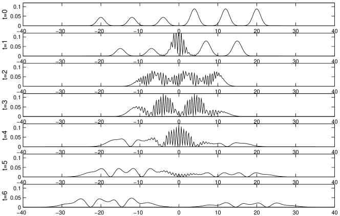
Fig. 4: Free evolution of a one-particle wavefunction consisting of six Gaussians, moving to the right and left, respectively.

The corresponding Bohmian trajectories, beeing solutions to the velocity vector field $v$, show the peculiar non-intersection property (figure 5). Even “free” particles change their direction of motion along their paths. The starting points of the worldlines are sampled according to $|\Psi_{0}|^{2}$.

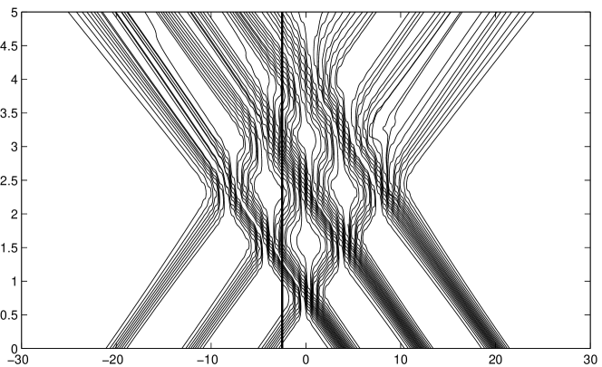
Fig. 5: Bohmian trajectories

We place a point detector $D$ at $x=-2.5$. The corresponding arrival time distribution is gained with the method of proposition 4. It shows areas of non-increasing arrival time probability, which correspond to times, during which already detected particles enter D for a second, third, etc. time, and therefore do not contribute to $P(t)$ anymore. Figure 6 illustrates this phenomenon and the technical procedure of proposition 4.

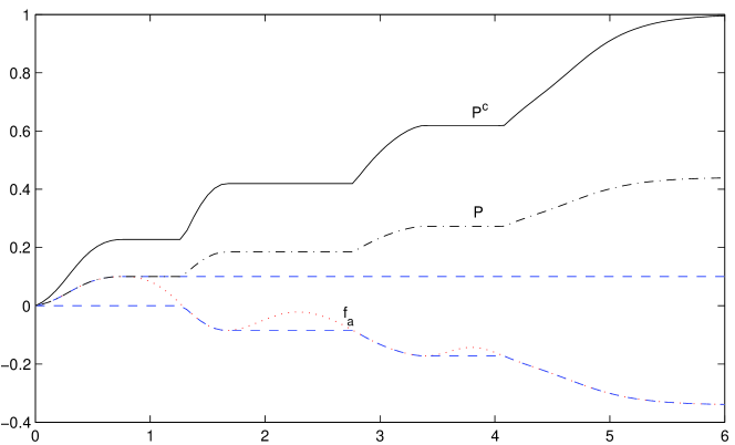
Fig. 6: $f_{a}$ (dotted line), $\max\{f_{a}(s)/\;0\leq s\leq t\}$, $-\max\{-f_{a}(s)/\;0\leq s\leq t\}$ (upper and lower dashed lines), the detection probability function $P$ (dashed-dotted line) and the conditional arrival time distribution $P^{c}$ (solid line).

5.2 The potential barrier

Terms as arrival-, delay- or dwell-times, etc in the literature are often connected to scattering states of one-dimensional potential barriers. For reviews of the subject see [12, 13, 14]. We apply equation (6) to a situation like that.

Now the evolution of our wavefunction $\Psi$ is given by the Schrödinger equation

$$\textrm{i}\partial_{t}\Psi=\left[-\frac{1}{2}\partial_{x}^{2}+\frac{1}{2}\big{(}\Theta(x-a)-\Theta(x-b)\big{)}\right]\Psi$$

with $a<b$ and $\Theta$ denoting the step function. The parameter reduction in this case can be achieved by taking the $t$-coordinates in units of $\frac{\hbar}{2V_{0}}$ and the $x$-coordinates in units of $\frac{\hbar}{\sqrt{2mV_{0}}}$, where $V_{0}$ is assumed to be the height of the potential barrier.

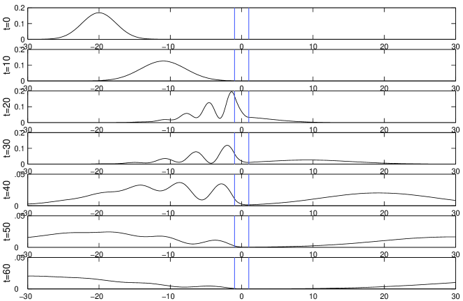
Fig. 7: Evolution of a Gaussian wave packet impinging on a potential barrier.

The initial gaussian wave packet $\Psi_{0}$ is placed sufficiently far to the left of the potential barrier (for the purpose that at time $t=0$ the interference effects due to the barrier are negligible). $\Psi$ is moving towards the barrier. The evolution of the wavefunction is illustrated in figure 7. Figure 8 shows the corresponding Bohmian trajectories sampled according to $|\Psi_{0}|^{2}$.

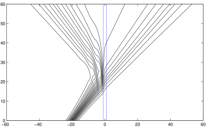
Fig. 8: Bohmian trajectories

We consider an extended detector occupying the spacetime region of the barrier from time $t=0$ onwards. As the wave packet is placed sufficiently far to the left of the barrier, the probability of a detection event at $t=0$ is negligible. Figure 9 shows, that $f_{b}$ is positive and monotonically increasing, which corresponds to a positive current density at the right edge of the potential barrier. Therefore $f_{b}$ does not contribute to an increase of the detection probability. As trajectories enter the detector from the left, $f_{a}$ at the left edge of the barrier increases up to a time $\tau_{r}$ when the first trajectory is reflected before entering the detection region. From $\tau_{r}$ onwards then part of the trajectories inside the barrier return to be finally reflected and therefore produce a negative current density at $x=a$, which leads to a small decrease of $f_{a}$. The resulting detection probability function $P$ and the conditional arrival time distribution $P^{c}$ are indicated in figure 9 by the dashed-dotted and solid lines, respectively.

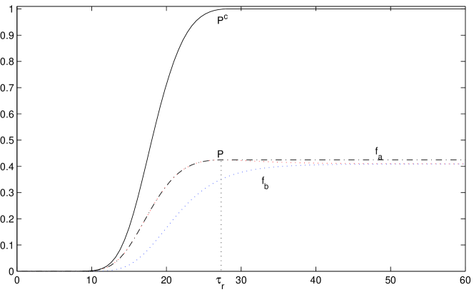
Fig. 9: $f_{a}$ and $f_{b}$ (upper and lower dotted lines), the detection probability function $P$ (dashed-dotted line) and the arrival time distribution $P^{c}$ (solid line) for the Gaussian wave packet impinging on a potential barrier.

5.3 The potential step

As a third numerical example we take the case of total reflection at a potential step at $x=0$. The wavefunction $\Psi$ is now the solution of the Schrödinger equation

$$\textrm{i}\partial_{t}\Psi=\left[-\frac{1}{2}\partial_{x}^{2}+\frac{1}{2}\Theta(x)\right]\Psi$$

with $\Theta$ again denoting the step function. The parameter reduction can be achieved analogously to the case of the potential barrier. Again the initial data $\Psi_{0}$ of $\Psi$ is taken to be a Gaussian wave packet placed to the left of the potential step at $t=0$ (figure 10).

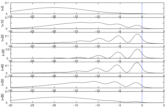
Fig. 10: Evolution of a Gaussian wave packet being totally reflected at a potential step at $x=0$.

This time we consider the situation, that at the time the detector is activated, some of the trajectories are already located inside the detection region $D$, located between $x=a$ and $x=b$ in front of the potential step, as illustrated in figure 11.

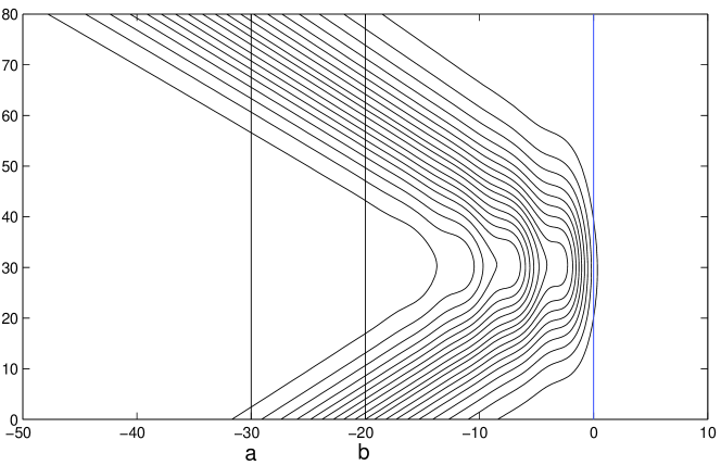
Fig. 11: Bohmian trajectories

The detection probability at time $t=0$ thus takes a value noticeably different from 0. As we have the case of total reflection, all the trajectories, which initially started to the right of $b$, eventually turn back and pass the detector at a later instance. Therefore almost all the trajectories pass $D$ at some time and the limit $\lim\limits_{s\to\infty}P(s)$ is approximately 1. The detection probability function and the conditional arrival time distribution thus coincide and are indicated by the solid line in figure 12.

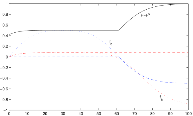
Fig. 12: $f_{a}$ and $f_{b}$ (dotted lines), $\max\{f_{a}(s)/\;0\leq s\leq t\}$ and $-\max\{-f_{b}(s)/\;0\leq s\leq t\}$ (upper and lower dashed lines), the detection probability function $P$ and the conditional arrival time distribution $P^{c}$ (solid line).

References

- [1] Misra B and Sudarshan E C G, Jour. Math. Phys. 18 (1997) 756
- [2] Grot N, Rovelli C and Tate R S, Phys. Rev. A 54 (1996) 4676
- [3] Muga J G and Leavens C R, Phys. Rep. 338 (2000) 353
- [4] Time in Quantum Mechanics , ed J G Muga et al, Berlin, Springer 2002
- [5] Leavens C R, Phys. Lett. A 178 (1993) 27
- [6] McKinnon W R and Leavens C R, Phys. Rev. A 51 (1995) 2748
- [7] Damborenea J A, Egusquiza I L, Hegerfeldt G C and Muga J G 2002 Phys Rev A 66 052104
- [8] Daumer M, Dürr D, Goldstein S and Zanghi N, Jour. Stat. Phys. 88 (1997) 967
- [9] Grübl G and Rheinberger K, Jour. Phys. A 35 (2002) 2907
- [10] Berndl K, Daumer M, Dürr D, Goldstein S, Zanghi N, Nuovo Cimento 110B (1995) 737
- [11] Loève M, Probability Theory, Princeton, Van Nostrand 1963; especially section 7,8 and 11.
- [12] Hauge E H and Støvneng J A, Rev. Mod. Phys. 61 (1989) 917
- [13] Olkhovsky V S and Recami E, Phys. Rep. 214 (1992) 339
- [14] Olkhovsky V S and Recami E, J. de Physique-I 5 (1995) 1351