Two-component Fermi gas in a Harmonic Trap

Abstract

We consider a mixture of two-component Fermi gases at low temperature. The density profile of this degenerate Fermi gas is calculated under the semiclassical approximation. The results show that the fermion-fermion interactions make a large correction to the density profile at low temperature. The phase separation of such a mixture is also discussed for both attractive and repulsive interatomic interactions, and the numerical calculations demonstrate the exist of a stable temperature region $T_{c1}<T<T_{c2}$ for the mixture. In addition, we give the critical temperature of the BCS-type transition in this system beyond the semiclassical approximation.

I Introduction

Since the experimental realization of Bose-Einstein condensation in dilute gases of rubidium[1-4], sodium[5,6], lithium[7], and hydrogen[8], a great deal of interest in trapped ultra-cold atoms has concentrated on the topic of trapped degenerate Fermi gas. However, it is difficult to achieve a degenerate state for fermonic atoms, because the $s-$wave collisions between fermions in a same state are suppressed by the Pauli principle, and the $p-$wave scattering as well as the dipole-dipole magnetic interaction are very weak at low temperature. The successful demonstration of overlapping condensates in different spin states of rubidium [9,10] and sodium [11] open a door to study the degenerate fermionic gas, because we can cool down one component of a mixture by sympathetic cooling. Inspired by this observation a number of experiments has been conducted on systems of Bose-Fermi mixtures, and most recently, using two-component evaporative cooling strategy, DeMarco and Jin[12] have succeeded in cooling fermonic atom gas down to about 0.5 $T_{F}$(300$nK$, depends on the trapping frequencies and the number of the trapped atoms). Below this temperature quantum degeneracy behaves as a barrier to evaporative cooling and as a modification of the classical thermodynamics. For the experiment reported by Demarco and Jin[12], the atom ${}^{40}K$ were trapped in two magnetic sublevels, $|F=9/2,m_{F}=9/2\rangle$ and $|9/2,7/2\rangle$, this mixture of atoms states is metastable against $m_{F}$ which changes collisions at low temperature, therefore the atom in each state is separately conserved. In such a two-component mixture of trapped spin-polarized ${}^{40}K$ atoms, interactions between atoms in different hyperfine states are much larger than those among atoms in the same state. Indeed, under this approximations a relatively high temperature $T_{c}$ for a BCS-type phase transition was predicted[13-14].

The purpose of this paper is to examine the properties including normal and BCS-type phase transition of such trapped atoms. The normal state properties of such a system were studied under the semiclassical approximation in Ref.[15-18]. However, as the interactions between ${}^{40}K$ atoms in the two different hyperfine states are considerable strong, it is important to include the effect of these interactions in any realistic treatment of the system. The present paper extends the analysis of Ref.[13-18] by considering both the discrete nature of the trapped atom and the effects of the interactions among them.

The paper is organized as follows. In Sec.II, we analyze the influence of the trap potential and the interactions on the density profile of the trapped atomic gas. We show that the cloud of the trapped atoms is compressed (diluted) for the case of attractive(repulsive) interactions. The stability properties of the trapped two-component Fermi gases are considered in Sec.III, and in Sec.IV we investigate the BCS-type transition in the system by taking the discrete nature into account. We find that the discrete nature is indeed make sense, they decrease the BCS-type transition temperature. The results for the BCS-type transition are beyond the semiclassical approximation. Finally, we summarize our results in Sec. V.

II Density profile of a trapped interacting two-component Fermi gas

We consider a dilute gas which consists of interacting fermionic two-level atoms trapped in an external potential $V_{0}(r)$. As the gas is dilute, the interactions mainly happen through two-body collisions. Furthermore, because the $s-$wave scattering length between fermions in a state is suppressed, and the p-wave scattering is greatly reduced due to the presence of the centrifugal barrier, we may neglect the interactions between fermions in the same hyperfine state and only consider the s-wave scattering between the fermions in different hyperfine states. Under this consideration, the system is then described by the following Hamiltonian

$$H = H_{1}+H_{2}+H_{int},$$

$$H_{i} = \int dr\psi_{i}^{\dagger}(\frac{p^{2}}{2m}-\mu+V_{0}(r))\psi_{i}(r),(i=1,2)$$

$$H_{int} = v_{0}\int drdr^{{}^{\prime}}\psi_{1}^{\dagger}(r)\psi_{2}^{\dagger}(r^{{}^{\prime}})\delta(r-r^{{}^{\prime}})\psi_{2}(r^{{}^{\prime}})\psi_{1}(r),$$ (1)

where $m$ is the mass of one fermion, and the interatomic potential has been approximated by a constant potential $v_{0}\delta(r-r^{{}^{\prime}})$. $\psi_{i}(r)$ stands for the annihilation operator of a fermion at position $r$ in the hyperfine state $|i\rangle$, and it obeys the usual fermionic anticommutation rules. The trapping potential is for simplicity taken to be an isotropic harmonic oscillator potential $V_{0}(r)=\frac{1}{2}m\omega^{2}r^{2}$, and the trapping frequency is the same for each hyperfine state. In addition to what we stated above, we have assumed that the number of particles $N$ in each state is the same such that we only have one chemical potential $\mu$. As the critical temperature for a BCS-type transition is maximum when the number of particles in the two hyperfine state is equal[13,14], so this configuration has most experimental relevance. Indeed, in the experiment reported in Ref.[12], the number of the atoms in state $m_{F}=9/2$ and $m_{F}=7/2$ are approximately equal. The noninteracting case is achieved by setting $v_{0}=0$; this limit has been discussed in ref.[15,16,18] for one component Fermi gas within the semiclassical approximation. In this section, we are interested in the effect of the interaction and the trapping potential on the density profile under the semiclassical approximation. We can, therefore, ignore any pairing correlations leading to BCS-type transition, and use the mean field Hamiltonian

$$H_{m1} = (\frac{p^{2}}{2m}-\mu+\frac{1}{2}m\omega^{2}r^{2})+v_{0}\langle\psi_{2}^{\dagger}(r)\psi_{2}(r)\rangle,$$

$$H_{m2} = (\frac{p^{2}}{2m}-\mu+\frac{1}{2}m\omega^{2}r^{2})+v_{0}\langle\psi_{1}^{\dagger}(r)\psi_{1}(r)\rangle,$$ (2)

this equation comes from eq.(1) straightforwardly. Here, $H_{mi}$ describes the effective Hamiltonian for component $i$. $\langle\psi_{i}^{\dagger}(r)\psi_{i}(r)\rangle$ is the standard Hartree-Fock result for a hard sphere interaction model. In order to get some analytical results, we study the density profile here within the semiclassical approximation, it is given from eq.(2) that

$$n_{i}(r)=\frac{3}{2}(\frac{m}{2\pi\hbar^{2}})^{\frac{3}{2}}\beta^{-\frac{5}{2}}f_{\frac{5}{2}}(z_{i})(i=1,2),$$ (3)

where $\beta=1/k_{B}T,$ $k_{B}$ is Boltzmann’s constant. $z_{1}=exp(\beta(\mu-v_{0}n_{2}(r)-V_{0}(r))),$ and $z_{2}=exp(\beta(\mu-v_{0}n_{1}(r)-V_{0}(r)))$ are called local fugacity[19] for component 1 and 2, respectively. $\mu$, the chemical potential for the atom, is determined through $N_{i}=\int drn_{i}(r)$. Before we present the density profile of the two-component Fermi gases, we consider a range of parameters for relevant experiment reported in Ref.[12]. The potentials for the centre-of-mass motion of a single atom in the hyperfine state can be approximated as a cylindrically symmetric harmonic potential with an axial frequency of $\omega_{z}=2\pi\times 19.5Hz$ and a variable radial frequency, which can be varied from $\omega_{r}=2\pi\times 44Hz$ to $2\pi\times 370Hz$. With the temperature being cooled down, the quantum statistical properties of the trapped gases become more evident, and at temperature $T\sim 0.5T_{F}\sim 300nK,$ the effect of Fermi-Dirac statistical are observed in the momentum distribution of the gas. With these parameters, it is evident that $\hbar\omega/k_{B}T<<1$, i.e., the semiclassical approximation is a good approach to the realistic case. (This does not indicate that the semiclassical approximation holds well at the temperature where BCS-type transition occurs) As the gas is dilute, we can expand $n_{i}(r)$ up to first order of the coupling constant $v_{0}$, one gives

$$n_{a}(r)=\frac{3}{2}(\frac{m}{2\pi\hbar^{2}})^{\frac{3}{2}}\beta^{-\frac{5}{2}}(f_{\frac{5}{2}}(z_{a}^{0})-v_{0}(z_{a}^{0})^{2}f_{\frac{3}{2}}(z_{a}^{0})\beta n_{b}^{0}),$$ (4)

where

$$n^{0}_{b}(r)=\frac{3}{2}(\frac{m}{\pi\hbar^{2}})^{\frac{3}{2}}\beta^{-\frac{5}{2}}f_{\frac{5}{2}}(z_{b}^{0}),$$

and $a,b=1,2$, $z_{a}^{0}=z_{b}^{0}=exp(\beta(\mu-\frac{1}{2}m\omega^{2}r^{2})).$ The result shows that for $v_{0}<0$, i.e., attractive interaction, the cloud of particles is compressed as compared to the noninteracting result. Because a high density of particles increases the critical temperature for a BCS-type transition, this effect favors the formation of the superfluid state[13].

III Stability properties of a trapped two-component Fermi gas

Since the experimental realization of the two-component condensate. Most of the theoretical works concerning multicomponent condensates[20-26] has been devoted to systems of two Bose condensates and Bose-Fermi mixture[27-30]. However, other systems are of fundamental interest, one of these is two-component trapped Fermi gas. In fact, by using the sympathetic cooling, the fermionic atoms in different hyperfine states has been cooled down to $300nK$, and the quantum statistical effect in this system has been reported[12].

For the two-component fermion system, the thermodynamical properties are trivial if there are not interaction between them. But in this case the sympathetic cooling scheme can not make effect and the degenerate fermions in a trapped potential can not been achieved. The thermodynamical properties may be changed when the interactions within and between the two hyperfine levels turn on. Then a new phenomenon, the phase separation, may occur in this system. For a homogeneous fermion mixture system, the Helmholts free energy can be written as[31]

$$\beta F = -\frac{2V}{\lambda_{2}^{3}}f_{\frac{5}{2}}(z_{2})+2a_{2}N_{2}\rho_{2}\lambda_{2}^{2}$$ (5)

$$- \frac{2V}{\lambda_{1}^{3}}f_{\frac{5}{2}}(z_{1})+2a_{1}\rho_{1}N_{1}\lambda_{1}^{2}+a_{12}(\lambda_{1}^{2}+\lambda_{2}^{2})N_{2}N_{1}/V,$$

where index 2 refers to the fermionic component in level $|9/2,7/2\rangle$, whereas index 1 stands for them in $|9/2,9/2\rangle$, $N_{i}$ is the number of particles in component $i$, $\lambda$ denotes the thermal wave length of the atoms, $f_{n}(z)$ represents the Fermi integral, $a_{i}$ and $a_{ij}$ denote the coupling constants. From eq.(5) we obtain the chemical potential for each component straightforwardly,

$$\beta\mu_{1} = \beta\mu_{1}^{0}+4a_{1}\rho_{1}\lambda_{1}^{2}+a_{12}(\lambda_{1}^{2}+\lambda_{2}^{2})N_{2}/V,$$

$$\beta\mu_{2} = \beta\mu_{2}^{0}+4a_{2}\rho_{2}\lambda_{2}^{2}+a_{12}(\lambda_{1}^{2}+\lambda_{2}^{2})N_{1}/V,$$ (6)

where $\mu_{i}^{0}$ are the chemical potentials of ideal gas. There are three terms in each chemical potential(6). The second term comes from the interaction within the component, while the third term is from the interaction between the fermions in different levels. As known, an homogenous binary mixture is stable only when the symmetric matrix $\hat{\mu}$ given by

$$\hat{\mu}=\left[\matrix{\frac{\partial\mu_{1}}{\partial\rho_{1}}&\frac{\partial\mu_{1}}{\partial\rho_{2}}\cr\frac{\partial\mu_{2}}{\partial\rho_{1}}&\frac{\partial\mu_{2}}{\partial\rho_{2}}}\right]$$ (7)

is non-negatively definite. In other words, all eigenvalues of matrix $\hat{\mu}$ given in eq.(7) are non-negative. Mathematically, for homogenous two-component fermions the stability conditions are

$$\frac{\partial\mu_{1}}{\partial\rho_{1}}\geq 0,\frac{\partial\mu_{2}}{\partial\rho_{2}}\geq 0,$$ (8)

and

$$det\left[\matrix{\frac{\partial\mu_{1}}{\partial\rho_{1}}&\frac{\partial\mu_{1}}{\partial\rho_{2}}\cr\frac{\partial\mu_{2}}{\partial\rho_{1}}&\frac{\partial\mu_{2}}{\partial\rho_{2}}}\right]\geq 0.$$ (9)

For ideal gas, we have $\rho_{1}=\frac{1}{\lambda_{1}^{3}}f_{\frac{3}{2}}(z_{1}),$ and $\rho_{2}=\frac{1}{\lambda_{2}^{3}}f_{\frac{3}{2}}(z_{2}),$ this leads to

$$\beta\frac{\partial\mu_{2}^{0}}{\partial\rho_{2}}=\frac{\lambda_{2}^{3}}{f_{\frac{1}{2}}(z_{2})},\,\beta\frac{\partial\mu_{2}^{0}}{\partial\rho_{2}}=\frac{\lambda_{1}^{3}}{f_{\frac{1}{2}}(z_{1})},$$ (10)

It follows from eqs (8) and (9) that

$$4a_{1}\lambda_{1}^{2}+\frac{\lambda_{1}^{3}}{f_{\frac{1}{2}}(z_{1})}\geq 0,$$ (11)

$$4a_{2}\lambda_{2}^{2}+\frac{\lambda_{2}^{3}}{f_{\frac{1}{2}}(z_{2})}\geq 0,$$ (12)

and

$$Z(T,a_{12}) = (4a_{1}\lambda_{1}^{2}+\frac{\lambda_{1}^{3}}{f_{\frac{1}{2}}(z_{1})})(4a_{2}\lambda_{2}^{2}+\frac{\lambda_{2}^{3}}{f_{\frac{1}{2}}(z_{2})})$$ (13)

$$- a_{12}^{2}(\lambda_{1}^{2}+\lambda_{2}^{2})^{2}\geq 0.$$

Now, we discuss the stability of this system with repulsive interactions. The case with attractive interactions will be discussed in the next section. It is obvious that the stability condition (11) and (12) hold always for $a_{1}>0$, $a_{2}>0$. We would like to point out that the stability conditions (11-13) do not involve the densities of the both components. At first glance, this seems to be confusion. In fact, there is no contradiction. One can demonstrate that at low density the Helmholtz free energy of the gas reduce to a quadratic form in $N_{1}$ and $N_{2}$. To have a minimum, this form should be positive definite, i.e., $\mbox{det}||\frac{\partial^{2}F}{\partial N_{1}\partial N_{2}}||\geq 0.$ Therefore, the corresponding stability criterion involves only density-independent constants. This criterion is similar to the stability conditions for two-component Bose-Einstein condensate in a trapped ultra-cold gas[23,24,33-37]. When $T\rightarrow\infty,\lambda_{i}\rightarrow 0$, hence $Z(T,a_{12})\sim\frac{1}{\rho_{1}\rho_{2}}$. Thus at high temperature, the homogeneous binary gas mixture is always stable and no phase separation occur. The quantity $Z(T,a_{12})$ as a function of the temperature is illustrated in Fig.1. We see from Fig.1 that the system is always stable when $T\rightarrow 0$ and $T\rightarrow\infty$, and the system is unstable for $T_{c1}<T<T_{c2}$. In particular, $T_{c1}$ and $T_{c2}$ depend on $a_{12}$ , the scattering length for fermions in different states. As $a_{12}$ decreases, $T_{c1}$ tends to $T_{c2}$ (going from fig.1-a to fig.1-b). /

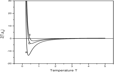
Figure 1: $Z(T,a_{12})$ vs. temperature $T$. The coupling constant $a_{12}$ is different for Fig.1-a and Fig.1-b. a:$a_{12}=0.5$, b:$a_{12}=0.2$. The parameters for Fig.1c are the same as those in Fig.1-b, but for the inhomogeneous case.

We would like to note that, the stability condition depends only on $|a_{12}|$, so the fermions with $a_{12}$ and $-a_{12}$ have the same stability condition. And the stability discussed above is only a result of interactions among different components.

Until now, we considered only a homogeneous Fermi gas mixture at finite temperature. In practise, however, experiments with ultracold atoms are performed by trapping and cooling atoms in an external potential that can be generally modeled by an isotropic harmonic oscillator $V(r)=\frac{m}{2}\omega^{2}r^{2}$, where $\omega$ is the trapping frequency. An exact criterion for the stability of an inhomogeneous Fermi-Fermi mixture should involve calculating the Helmholtz free energy. Fortunately, in the system considered here it is a good approach to take use of the semiclassical approximation, which treats the atoms as a local homogeneous system. This approximation requires that the level spacing $\hbar\omega$ of the trapping potential is much smaller than the Fermi energy. Of course, the semicalssical approximation always breaks down at the edge of the gas cloud where the density vanishes and the effective Fermi energy becomes zero. In this approximation, the stability conditions can still be calculated by means discussed above, with the understanding that the effective chemical potentials are spatially dependent through

$$\mu_{1}=\mu_{1}^{0}-\frac{1}{2}m\omega^{2}r^{2},\,\mu_{2}=\mu_{2}^{0}-\frac{1}{2}m\omega^{2}r^{2}.$$

In this sense, the stability condition is the same as given in eq.(13) but replacing $z_{i}(i=1,2)$ by

$$\tilde{z}_{1}=z_{1}e^{-\frac{\beta}{2}m\omega^{2}r^{2}},\mbox{\ \ and\ \ }\tilde{z}_{2}=z_{2}e^{-\frac{\beta}{2}m\omega^{2}r^{2}}.$$

As shown in Fig.1-c, the region of temperature in which the system is unstable becomes narrow as compared to the homogeneous case($r=0$).

IV BCS-type transition in trapped two-component Fermi gas

The achievement of atomic Bose-Einstein condensation has induced an experimental growth of interest in the properties of ultracold dilute quantum gases. Of particular interest now is the physics of trapping and cooling of fermionic atoms. Indeed the prospect of superfluidity with dilute atomic vapors has already been studied within the semiclassical approximation by several groups [13,14,38,39]. Because the semiclassical approximation is not of fundamental quantum physics, we will extend the analysis under the semiclassical approximation by including the discrete nature of the trapped atom in this section.

Let us consider two species of fermions in a trap, which interact with each other by two-body collisions( $s-$ wave scattering). The Hamiltonian describing such a system is given by eq.(1). The two species of fermions correspond to the trapped atoms in two hyperfine levels $|1\rangle=|9/2,9/2\rangle$ and $|2\rangle=|9/2,7/2\rangle$. Expanding $\psi^{\dagger}_{\alpha}(r)(\alpha=1,2)$ by

$$\psi_{\alpha}^{\dagger}(r)=\sum_{n}a_{n\alpha}^{\dagger}\phi_{n}^{*}(r),$$ (14)

where $a_{n\alpha}^{\dagger}$ creates one particle in state $|\alpha n\rangle=|\alpha\rangle\otimes|n\rangle,$ which satisfies

$$(-\frac{\hbar^{2}}{2m}\nabla^{2}+\frac{1}{2}m\omega^{2}r^{2})|\alpha n\rangle=\varepsilon_{n\alpha}|\alpha n\rangle,$$ (15)

the Hamiltonian in eq.(1) becomes

$$H=\sum_{\alpha n}\varepsilon_{\alpha n}a_{\alpha n}^{\dagger}a_{\alpha n}+\sum_{i,j,m,n}V_{ijmn}a_{i\alpha}^{\dagger}a_{j-\alpha}^{\dagger}a_{m-\alpha}a_{n\alpha},$$ (16)

where $V_{ijmn}=v_{0}\int drdr^{{}^{\prime}}\delta(r-r^{{}^{\prime}})\phi_{i}^{*}(r)\phi_{j}^{*}(r^{{}^{\prime}})\phi_{m}(r^{{}^{\prime}})\phi_{n}(r)$ and $\alpha$, $-\alpha$ denote the two hyperfine levels(say, for example, if $\alpha=|9/2,9/2\rangle$ , then $-\alpha=|9/2,7/2\rangle$). The next step in a mean-field treatment of the Hamiltonian in eq.(16) is to develop the operator product $\psi_{\alpha n}^{\dagger}\psi_{-\alpha n}^{\dagger}$ around their mean values by substituting

$$\psi_{\alpha n}^{\dagger}\psi_{-\alpha n}^{\dagger}=\langle\psi_{\alpha n}^{\dagger}\psi_{-\alpha n}^{\dagger}\rangle+\delta\psi_{\alpha n}^{\dagger}\psi_{-\alpha n}^{\dagger}.$$

To first order in the fluctuations, we are left with the effective mean-field Hamiltonian

$$H\simeq\sum_{\alpha n}\varepsilon_{\alpha n}a_{\alpha n}^{\dagger}a_{\alpha n}+\sum_{m}\Delta_{m}a_{\alpha m}^{\dagger}a_{-\alpha m}+\sum_{m}\Delta^{*}_{m}a_{\alpha m}a_{-\alpha m}.$$ (17)

Here $\Delta_{m}=(\Delta_{m}^{*})^{*}=\sum_{n}V_{mmnn}\langle a_{\alpha n}a_{-\alpha n}\rangle$ is the equilibrium value of the BCS order parameter. As the effective mean-field Hamiltonian in terms of the operators $a_{\alpha n}^{\dagger}$ and $a_{\alpha n}$ is non-diagonal, one can not directly calculate the expection value $\langle a_{\alpha n}^{\dagger}a_{\alpha n}\rangle$. This is, as usual, resolved by first applying a Bogoliubov transformation

$$b_{\alpha m}=u_{m}a_{\alpha m}+v_{m}a_{-\alpha m}^{\dagger},$$

$$b_{\alpha m}^{\dagger}=u_{m}a_{\alpha m}^{\dagger}+v_{m}a_{-\alpha m},$$ (18)

to diagonalize the Hamiltonian in eq.(17). After performing this unitary transformation, we require that the Hamiltonian in terms of the new quasiparticle operators $b_{\alpha m}$ and $b_{\alpha m}^{\dagger}$ has only diagonal elements, and furthermore we assume that these operators obey the usual anticommutation relations still. This determines the values of the yet unknown $u_{m}$ and $v_{m}$. The latter constraint requires that the constant $u_{m}$ and $v_{m}$ must satisfies the relations $|u_{m}|^{2}+|v_{m}|^{2}=1$ and the requirement of diagonality of the Hamiltonian after Bogoluibov transformation lead to $|v_{m}|^{2}=\frac{2}{1-\varepsilon_{m}/E_{m}}$ with $\varepsilon_{m}=\varepsilon_{\alpha m},$ $E_{m}=\sqrt{\Delta_{m}^{2}+\varepsilon_{m}^{2}}$. $E_{m}$ are eigenvalues of the Bogoluibov quasiparticles.

Using Bogoluibov transformation(18), the equilibrium value of the BCS order parameter is calculated easily, it is given that

$$\Delta_{n}=\sum_{m}V_{mmnn}\frac{\Delta_{m}}{E_{m}}tanh\frac{\beta}{2}E_{m}.$$ (19)

As usual, the order parameter does not depend on its index $m$. So we arrive at the gap equation

$$\sum_{m}V_{mmnn}\frac{1}{\sqrt{\varepsilon_{m}^{2}+\Delta^{2}}}tanh\frac{\sqrt{\varepsilon_{m}^{2}+\Delta^{2}}}{2k_{B}T}=1.$$ (20)

Setting $\Delta=0$, one finds the critical temperature $T_{c}$ as a function of the trapping frequency $\omega$[18]. The density $N(0)$ of atoms near the Fermi surface and the coupling constant $v_{0}=V_{mmnn}$,

$$1 = v_{0}N(0)ln(1.13\beta_{c}\hbar\omega)+v_{0}Bk_{B}T_{c}\frac{exp[\frac{\hbar\omega}{k_{B}T_{c}}]}{1+exp[\frac{\hbar\omega}{k_{B}T_{c}}]}$$ (21)

$$- \frac{1}{2}v_{0}Bk_{B}T_{c}-v_{0}Bk_{B}T_{c}ln(1+exp[\frac{\hbar\omega}{k_{B}T_{c}}])$$

$$+ v_{0}Bk_{B}T_{c}ln2,$$

where $B=\frac{3}{2(\hbar\omega)^{2}}$ and $\beta_{c}=\frac{1}{k_{B}T_{c}}.$ The first term in the right hand side of eq.(21) is just from the usual BCS theory, in other words, if the semiclassical approximation is a good approach to the theory or the discrete nature of the trap levels can be neglected, $T_{c}=\frac{\hbar\omega}{k_{B}}e^{-\frac{1}{v_{0}N(0)}}.$ The rest terms in the right hand side of eq.(21) are corrections of the discrete trap levels to the usual BCS theory.

This superfluid phase transition, which is similar to the BCS transition in a superconductor, might occur at very low temperature. At such low temperature, whether the semiclassical approximation holds depend on both the temperature and the trapping frequency. Hence we investigate here the BCS-type transition from the other aspect, beyond the semiclassical approximation. The results show that if the semiclassical approximation holds, i.e., $\hbar\omega/k_{B}T_{c}<<1$, the transition temperature is just the BCS one. Otherwise the effects of the discrete trap levels provide a negative correction to the transition temperature.

V Conclusion

In summary, we considered a Fermi gas occupying two hyperfine states trapped in a magnetic field. Atoms in different hyperfine levels can interact via $s-$wave scattering. Under the semiclassical approximation, we calculated and discussed the density profile for the trapped fermions. The purterbative results up to the first order of the coupling constant show that the density of the atom is compressed(diluted) as compared to the noninteracting case due to attractive (repulsive)interaction. We also investigate the mechanical and statistical stability of the two-component gas with interaction between the atoms in different hyperfine levels, and find that these interactions strongly affect the stability of the system at finite temperature. The regime $T_{c1}\leq T\leq T_{c2}$ in which the system is unstable depend on the strength of the interaction and the spatial atomic position. Furthermore, we consider the BCS-type transition beyond the semiclassical approximation, within which the most current literature study the superfluid state of trapped fermonic atoms. The results showed the transition temperature is a function of the trapped frequency, the coupling constant and, as usual, the density of the atoms near the Fermi surface. Neglecting the discrete nature of the trap levels, the transition temperature return to the BCS’s one, and the correction to $T_{c}$ is negative due to the discrete nature of the trapped atom.
ACKNOWLEDGEMENT:
We thank Prof. C. P. Sun, Prof. W. M. Zheng, Dr. Li You for their stimulating discussions. This work was supported by NNSF of China.

References

- (1) M.H.Anderson etal., Science 269(1995)198.
- (2) D.J.Han, R.H.Wynar, P.Courteille, and D.J.Heinzen, Phys. Rev. A 57(1998)R4114.
- (3) U.Ernst et al., Europhys. Lett. 41(1998)1.
- (4) T.Esslinger, I.Bloch, and T.W.Hansch, Phys. Rev. A 58(1998)R2664.
- (5) K.B.Davis etal. Phys. Rev. Lett. 75(1995)3969.
- (6) L.V.Hau etal. Phys. Rev. A 58(1998)R54.
- (7) C.C.Bradley etal., Phys. Rev. Lett. 75(1995)1687.
- (8) D.G.Fried etal., physics/9809017.
- (9) C.J.Myatt etal., Phys. Rev. Lett. 78(1997)586.
- (10) M.R.Matthews etal. Phys. Rev. Lett. 81(1998)243.
- (11) D.M.Stamper-Kurn etal., Phys. Rev. Lett. 80(1998)2027.
- (12) B.DeMarco, D.S.Jin, Science 285(1999)1703.
- (13) H.T.C.Stoof, M.Houbiers, C.A.Sackett, and R.G.Hulet, Phys. Rev. Lett. 76(1996)10.
- (14) M.Houbiers, R.Ferwerda, H.T.C.Stoof W.I. MaAlexander, C.A.Sackett, and R.G.Hulet Phys. Rev. A 56(1997)4864.
- (15) D.A.Butts and D.S.Rokhar, Phys. Rev. A 55(1997)4346.
- (16) J.Schneider and H.Wallis, Phys. Rev. A 57(1998)1253. M.Amoruso, C.Minniti, M.P. Tosi Eur. Phys. J. D. 8(2000)19.
- (17) G.M.Bruun, K.Burnett, Phys. Rev. A 58(1998)2427. G. Bruun, Y. Castin, R. Dum, K. Burnett, Eur. Phys. J. D 7(1999) 433. G. M.Bruun, C. W. Clark, J. Phys. B 33(2000) 3953.
- (18) X.X.Yi and J.C.Su, Physica Scripta 60(1999)117.
- (19) T.T.Chou, C.N.Yang, L.H.Yu, Phys. Rev. A 55(1997)1179.
- (20) T.L.Ho and V.B.Shenoy, Phys. Rev. Lett. 77(1996)3276.
- (21) B.D.Esry, C.H.Greene, P.B.James, Jr. and J.L.bohn, Phys. Rev. Lett. 78(1997)3594.
- (22) R. Graham and D.Walls, Phys. Rev. A 57(1998)484.
- (23) P.Öhverg and S. Stenholm, Phys. Rev. A 57(1998)1272.
- (24) H.Pu and N.P.Bigelow, Phys. Rev. Lett., 80(1998)1130.
- (25) H.Pu and N.P.Bigelow, Phys. Rev. Lett., 80(1998)1134.
- (26) D.Gordon and C.M.Savage, Phys. Rev. A 58(1998)1440.
- (27) N.Nygaard, K.Mlmer, Phys. Rev. A 59(1999)2974.
- (28) K.Mlmer, Phys. Rev. Lett. 80(1998)1840.
- (29) L.Vichi, M.Amoruso, A.Minguzzi, etal., cond-mat/9909150.
- (30) W.Geist, L.You, T.A.B.Kennedy, Phys. Rev. A 59(1999)1500.
- (31) C.E.D.G.Cohen, J.M.J.van Leeuwen, Physica 26(1960)1171.
- (32) E.P.Bashkin, A.V.Vagov, Phys. Rev. B 56(1997)6207.
- (33) P.öhberg, Phys. Rev. A59(1999)634.
- (34) C.K.Law, H.Pu, etal.Phys. Rev. Lett. 79(1997)3150.
- (35) H.Shi, Ph.D. thesis, Institute of Theoretical Physics, Academia Sinica, Peking, China 1998.
- (36) L.D.Landau and E.M.Lifshits, Statistical Physics(Pergamon New York, 1977), Part 1.
- (37) J.Schneider, H.Wallis, Phys. Rev. A 57(1997)1253.
- (38) M.A.Baranov and D.S.Petrov, Phys. Rev. A 58(1998)R801.
- (39) L.You and M.Marinescu, Phys. Rev. A 60(1999) 2324.