Quantum Limits of Stochastic Cooling of a Bosonic Gas

Abstract

The quantum limits of stochastic cooling of trapped atoms are studied. The energy subtraction due to the applied feedback is shown to contain an additional noise term due to atom-number fluctuations in the feedback region. This novel effect is shown to dominate the cooling efficiency near the condensation point. Furthermore, we show first results that indicate that Bose–Einstein condensation could be reached via stochastic cooling.

Ultracold atomic gases are generated by laser cooling laser-cooling , evaporative cooling evap-cooling or sympathetic cooling symp-cooling . These techniques have been successful in preparing Bose–Einstein condensed bec and Fermi degenerate fermi atomic gases. These states of matter have proven important in both the fundamental physics of weakly interacting many-body systems mott and in applications atom-laser ; bec-micro . Nonetheless, these cooling methods have some limitations. For example, laser cooling requires closed-cycle transitions, evaporative cooling leads to a loss of a significant fraction of the atoms, and sympathetic cooling requires careful selection of buffer species with sufficiently large scattering cross sections.

A much more general strategy that avoids these limitations is stochastic cooling stochastic-cooling . It is a Maxwell-demon strategy that uses information obtained from measurement to coherently reduce the energy of part of the system. Stochastic cooling is based on the repeated application of a feedback loop. The cooling is obtained by the combination of measurement and controlled Hamiltonian interaction during the feedback operation. The interaction provides an energy exchange with an external field and the preceeding measurement ensures the irreversibility of this exchange. In this way the feedback mechanism may be thought of as acting as a dissipative reservoir. Classically cooling occurs due to the extraction of information on the phase-space localization of particles, and its subsequent use to reposition the particles, leading to a phase-space compression stochastic-cooling .

In high-energy physics it has been employed for cooling the transverse degree of freedom of a particle beam stochastic-cooling . A measurement of the transverse momentum of a fraction of the particles is made. A control field sets the momentum to zero, which together with a subsequent remixing of the particles leads to phase-space compression and cooling of the transverse motion. Recently, stochastic cooling was proposed for trapped atoms and it was shown that both momentum measurement and shift could be realized by optical fields stochastic-raizen . The required remixing of atoms is provided here by the oscillation in the trap. Moreover, interactions between atoms, such as collisions, may provide a further enhancement of this remixing. Classical calculations for a 1D atomic gas showed a pronounced cooling effect stochastic-raizen , so that stochastic cooling may perhaps be an alternative to standard cooling methods.

However, to best of our knowledge, it is not yet known to what temperatures such a method eventually will cool the atoms and whether, for example, Bose–Einstein condensation can be reached. Technical heating effects, that are inherent in the proposed optical implementation, have been discussed stochastic-raizen . However, the fundamental limits of such a cooling method, due to the discreteness of atoms and their quantum correlations, seem to be unexplored. A reason for the lack of knowledge of these limits may be that many-atom correlations play a central role. The atoms cannot be treated as individual entities, which would considerably simplify a theoretical description, but require a quantum many-atom description wal-feedback .

Measurement in quantum mechanics always leads to a back-action in the conjugate variable, and one might expect that this will saturate the cooling at ultralow temperatures. It will be shown in this Letter that a further fundamental heating mechanism arises from the quantum fluctuations of the number of atoms in the feedback region. To reach ultralow temperatures, this heating has to be circumvented, which will be shown to be possible by the choice of the feedback region. We treat stochastic cooling in a fully quantum-field theoretical way and show initial results that indicate the possibility of reaching Bose–Einstein condensation.

The feedback loop of stochastic cooling consists of a measurement of the total momentum $\hat{P}_{w}$ of the atoms in the feedback region and a subsequent interaction in the same spatial region that compensates for the observed value $P$, i.e., shifts the total momentum to zero. The spatial region where atoms are subject to the feedback is defined by the beam of a laser field that implements the measurement and subsequent shift, cf. Ref. stochastic-raizen . For simplicity we consider the case where the laser beam is aligned along the $z$ axis and the beam waist $w$ shall be a step-like function in the $xy$-plane, cf. Fig. 1.

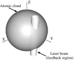
Figure 1: Geometry of the feedback setup. The laser beam is aligned along the $z$ axis, it determines the size of the feedback region.

Note that in $z$-direction no spatial restriction is assumed.

The measurement and subsequent shift shall occur without time delay and on timescales much smaller than the intrinsic timescale of the system $1/\omega_{0}$, where $\omega_{0}$ is the trap frequency of the 3D isotropic, harmonic potential. Then the entire feedback loop approximately acts instantaneously in time. Furthermore, we take into account the resolution $\sigma$ of the measurement of momentum $\hat{P}_{w}$, that is determined by external optical fields implementing the measurement.

The feedback acts on the many-atom density operator $\hat{\varrho}$ as

$$\hat{\varrho}_{+}=\int\!dP\,\hat{U}(P)\,\hat{M}(P\!-\!\hat{P}_{w})\,\hat{\varrho}_{-}\,\hat{M}^{\dagger}(P\!-\!\hat{P}_{w})\,\hat{U}^{\dagger}(P),$$ (1)

where $\hat{\varrho}_{\mp}$ are the many-atom density operators before ($-$) and after ($+$) the feedback. The measurement is described by the positive operator-valued measure $\hat{M}$, where $|M(P)|^{2}$ is a Gaussian of width $\sigma$. The unitary operator $\hat{U}(P)\!=\!\exp[iP\hat{Q}_{w}]$ implements the subsequent shift of the measured momentum $P$ to zero remark . The final density operator is found by averaging over all possible measurement outcomes.

Using the bosonic atom-field operator $\hat{\phi}({\mathbf{r}})$ with commutator $[\hat{\phi}({\mathbf{r}}),\hat{\phi}^{\dagger}({\mathbf{r}}^{\prime})]\!=\!\delta^{(3)}({\mathbf{r}}\!-\!{\mathbf{r}}^{\prime})$, the measured total momentum $\hat{P}_{w}$ and the center-of-mass $\hat{Q}_{w}$ of atoms in the feedback region are

$$\hat{P}_{w} = \int_{w}\!\!dA\int\!dz\,\hat{\phi}^{\dagger}({\mathbf{r}})\,(-i\partial_{z})\,\hat{\phi}({\mathbf{r}}),$$ (2)

$$\hat{Q}_{w} = \frac{1}{N_{\rm e}}\int_{w}\!\!dA\int\!dz\,\hat{\phi}^{\dagger}({\mathbf{r}})\,z\,\hat{\phi}({\mathbf{r}}),$$ (3)

where $dA$ is integrated over the beam waist $w$. Their commutator is $[\hat{Q}_{w},\hat{P}_{w}]\!=\!i\hat{N}_{w}/N_{\rm e}$, where the operator of the number of atoms in the feedback region is

$$\hat{N}_{w}=\int_{w}\!\!dA\int\!dz\,\hat{\phi}^{\dagger}({\mathbf{r}})\,\hat{\phi}({\mathbf{r}}).$$ (4)

Note that in Eq. (3) the estimated number of atoms $N_{\rm e}$ is used and not the proper operator $\hat{N}_{w}$: Since, roughly speaking, in the Schrödinger picture $\hat{U}(P)\!=\!\prod_{i}\exp(iP/N_{\rm e}\hat{q}_{i})$, where $\hat{q}_{i}$ is the coordinate of the $i$th atom, each atom is shifted by $-P/N_{\rm e}$. That is, since the true atom number is unknown — it is not measured — an estimate for the atom number, $N_{\rm e}$, has to be employed for properly shifting each atom’s momentum.

For cooling we are interested in the average energy that is subtracted by the feedback from the set of non-interacting atoms,

$$\Delta E=\langle\hat{H}\rangle_{+}-\langle\hat{H}\rangle_{-},$$ (5)

Here $\hat{H}$ is the Hamiltonian of the atoms in the harmonic trap potential and $\langle\ldots\rangle_{\pm}\!=\!{\rm Tr}(\hat{\varrho}_{\pm}\ldots)$. After a detailed calculation, using the results of Ref. wal-feedback , we find that $\Delta E$ consists of both cooling and heating terms.

Firstly, consider an expansion of the kinetic energy of the center of mass of the atoms in the feedback region, around the estimated atom number $N_{\rm e}$:

$$\hat{P}_{w}^{2}/(2m\hat{N}_{w})=\hat{P}_{w}^{2}/(2mN_{\rm e})(1\!-\!\delta\hat{N}_{w}/N_{\rm e}\!+\!\ldots),$$ (6)

where $\delta\hat{N}_{w}\!=\!\hat{N}_{w}\!-\!N_{\rm e}$. Following Ref. wal-feedback we find that only the zeroth- and first-order terms of this expansion appear in the energy change $\Delta E$: the expectation values of higher-order corrections exactly cancel each other. The leading term represents the cooling of the system by feedback. For this term, the energy removed is $-\langle\hat{P}_{w}^{2}\rangle_{-}/(2mN_{\rm e})$. With $m$ being the atomic mass, $N_{\rm e}m$ is the estimated total mass of the atoms in the feedback region, and $\hat{P}_{w}$ is their total momentum. Thus this is the negative (estimated) kinetic energy of the center-of-mass of the atoms in the feedback region. According to (2), this term contains atom-atom correlations of the form $\langle\hat{\phi}^{\dagger}({\bf r}_{1})\hat{\phi}({\bf r}_{2})\hat{\phi}^{\dagger}({\bf r}_{3})\hat{\phi}({\bf r}_{4})\rangle$ — a clear indication that in the quantum regime stochastic cooling cannot be described as a single-atom problem.

The first-order correction in Eq. (6) is found to give rise to a heating contribution to $\Delta E$ of the form $\langle\delta\hat{N}_{w}\hat{P}_{w}^{2}\rangle_{-}/(2mN_{\rm e}^{2})$. From Eq. (6) it can be seen, that this heating is due to non-optimal shifts of total momentum produced by atom-number fluctuations around the estimated value $N_{\rm e}$. Another way to see this is to consider a many-atom quantum state $|\Psi\rangle$ after a perfect measurement ($\sigma\!=\!0$) of $\hat{P}_{w}$ with outcome $P$. It shall also be an eigenstate of $\hat{N}_{w}$ with $N$ atoms in the feedback region, i.e., $|\Psi\rangle\!=\!|P,N\rangle$. After the momentum shift the state becomes $\hat{U}(P)\,|P,N\rangle\!=\!|P(1\!-\!N/N_{\rm e}),N\rangle$. That is, the momentum will be shifted to zero only if $N_{\rm e}\!=\!N$. Given that the system in general is in a state of imprecise atom number, choosing $N_{\rm e}\!=\!\langle\hat{N}_{w}\rangle$ will only produce the correct momentum shift on average. Therefore, atom-number fluctuations in the feedback region are transferred into momentum fluctuations, that lead to the observed residual kinetic energy. This poses a fundamental limit to the perfect operation of the feedback loop and thus to stochastic cooling .

Moreover, since a measurement is involved in the control loop, $\Delta E$ contains also measurement-induced heating terms: Since the total momentum is measured with resolution $\sigma$, this fluctuations of the total momentum leads to a residual kinetic energy of the center of mass of the atoms in the feedback region. Together with the correction factor $\langle\hat{N}_{w}\rangle_{-}/N_{\rm e}$ that accounts for the difference between estimated and average atom number, the resulting heating term is $\sigma^{2}/(2mN_{\rm e})\!\times\!\langle\hat{N}_{w}\rangle_{-}/N_{\rm e}$. Clearly a measurement of total momentum with resolution $\sigma$ induces back-action noise $\propto\sigma^{-1}$ into the center of mass of the measured atoms. This noise leads to an increase in potential energy (i.e. heating) of the center of mass in the harmonic trap, which is found to be $mN_{\rm e}\omega_{0}^{2}/(8\sigma^{2})\!\times\!\langle\hat{N}_{w}\rangle_{-}/N_{\rm e}$. Given these contributions, the total change of energy due to a single feedback operation is then

$$\Delta E=\left(\frac{\sigma^{2}}{2mN_{\rm e}}\!+\!\frac{mN_{\rm e}\omega^{2}_{0}}{8\sigma^{2}}\right)\!\frac{\langle\hat{N}_{w}\rangle_{-}}{N_{\rm e}}+\frac{\langle\delta\!\hat{N}_{w}\hat{P}_{w}^{2}\rangle_{-}}{2mN_{\rm e}^{2}}-\frac{\langle\hat{P}_{w}^{2}\rangle_{-}}{2mN_{\rm e}}.$$ (7)

To achieve optimal cooling $\Delta E$ should be as negative as possible which is achieved by minimizing the heating terms. The optimal measurement resolution, $\sigma_{\rm opt}\!=\!\Delta p_{0}\sqrt{N_{\rm e}}$, minimizes the measurement-induced heating [first term in Eq. (7)] to $\frac{1}{3}E_{0}\langle\hat{N}_{w}\rangle_{-}/N_{\rm e}$, where $E_{0}$ is the ground-state energy of a single atom remark . Choosing this value, the squared measurement resolution per atom equals the squared ground-state momentum uncertainty of a single atom, $\Delta p_{0}$. Since the number of atoms in the feedback region changes with temperature, the estimate $N_{\rm e}$ should have a temperature dependence. Thus $\sigma_{\rm opt}$ should be adapted during the cooling process, if possible, to provide maximum cooling. For further optimisation the size and location of the feedback region in the $xy$-plane (cf. Fig. 1) is of major importance. Here we consider only particular cases; a more detailed study of the optimization will be presented elsewhere. In particular, we focus on temperatures near the condensation point, to demonstrate that in principle Bose–Einstein condensation can be reached with stochastic cooling.

We have calculated the expectation values in Eq. (7) using the grand-canonical ensemble for a system at temperature $T$ and with average total number of atoms $N_{\rm tot}$. In this way we obtain the dependence of $\Delta E$ on the temperature for fixed $N_{\rm tot}$, as shown in Fig. 2 for $N_{\rm tot}\!=\!10^{6}$ atoms.

Figure 2: Energy change in units of $E_{0}$ versus temperature. $N_{\rm tot}\!=\!10^{6}$, size of feedback region in $x$, $y$ directions is $\Delta q_{0}$, locations are: centered (solid), shifted out of center by $5\!\times\!\Delta q_{0}$ (dashed).

If the feedback region is centered with respect to the trap potential, it has substantial overlap with the condensate wavefunction. In this case (solid curve), when the temperature is gradually decreased, there is a sudden change from cooling to heating at the condensation temperature $T_{0}$. This effect is due to dramatic atom-number fluctuations of the condensate fraction at temperatures close to the phase transition . These fluctuations lead to a substantial heating due to the second term in Eq. (7).

This problem can be avoided by choosing a feedback region that has no spatial overlap with the nascent condensate and is thus not affected by its large atom-number fluctuations. In this case the energy removed per step gradually diminishes below $T_{0}$, though cooling still takes place (dashed curve). On the other hand, the energy subtraction per step at $T\!\gg\!T_{0}$ is slightly smaller than for a centered feedback region. An advantageous strategy is therefore to gradually move the feedback region out of the trap center when approaching the condensation temperature.

Our present results lead us to the conclusion that neither quantum measurement effects nor the lack of knowledge of the precise number of atoms in the feedback region in principle prevent Bose–Einstein condensation by stochastic cooling. However, we have said nothing about the speed at which condensation may be reached. A conclusive answer on this issue requires that the cooling rate be dynamically calculated using the method described in Ref. wal-feedback . For now we proceed with an equilibrium approach that represents a worst-case scenario: Starting at temperature $T_{i}$ we calculate the energy subtraction $\Delta E(T_{i})$, and thus a new average energy. From this energy a new temperature $T_{i+1}$ is obtained by assuming the equilibration of the system during the free evolution after the feedback. That is, we assume that due to collisions the atoms exchange energy and re-establish a new equilibrium state. Iterating this calculation many times we obtain the dependence of temperature on the number of feedback operations, as depicted in Fig. 3.

Figure 3: Temperature $T$ (in $\mu$K) versus number of feedback operations $n$. Parameters as in Fig. 2, $\omega_{0}/(2\pi)\!=\!500$Hz. Solid (dashed) curve corresponds to centered (non-centered) feedback region, doted line indicates $T_{0}$.

Starting with a temperature of $7.6\,\mu$K, condensation is reached after about $10^{7}$ feedback operations. Again a feedback region outside the trap center is advantageous when reaching $T_{0}$ (dashed curve).

In a realistic experiment stochastic cooling is performed without waiting for re-equilibration between feedback operations . Then non-vanishing coherent amplitudes of the momentum $\langle\hat{P}_{w}\rangle$ will appear depending on the oscillation phase, i.e., the (randomly chosen) time of the subsequent feedback operation. Since $\langle\hat{P}_{w}^{2}\rangle\!=\!\langle(\Delta\hat{P}_{w})^{2}\rangle\!+\!\langle\hat{P}_{w}\rangle^{2}$, the feedback then not only reduces momentum fluctuations $\langle(\Delta\hat{P}_{w})^{2}\rangle$, as for a thermal state, but also subtracts the energy due to the non-equilibrium coherent amplitudes $\langle\hat{P}_{w}\rangle^{2}$ [cf. Eq. (7)]. The latter leads to additional energy subtractions as compared to our equilibrium approach. One can thus expect a much faster cooling process, so that our results (cf. Fig. 3) represent the upper limit of the required number of feedback operations.

Our calculations have shown that increasing the size of the feedback region further increases the cooling efficiency. Unfortunately, for enlarged feedback regions an increased number of trap levels is required, which presently runs into limitations of our numerics. For finding optimal strategies and parameter ranges of stochastic cooling we intend to implement in the near future a dynamical calculation wal-feedback . Then the dependence of the cooling rate on size and location of the feedback region can be studied in full detail.

It is worth noting, that the considered feedback regions could be easily realized in experiment by application of optical fields stochastic-raizen . The ground-state position variance of sodium atoms is approximately $\Delta q_{0}\!=\!0.6\mu{\rm m}$ for a trap of frequency $\nu\!=\!500$Hz. Beam waists of externally applied laser fields, that implement measurement and shift, can be chosen in a wide range limited only by optical wavelengths, which are much smaller than $\Delta q_{0}$. Thus sizes of the feedback region much smaller and much larger than $\Delta q_{0}$ could be realized.

Note also, that the geometry used here is different from that in Ref. stochastic-raizen . Raizen et al. considered a one-dimensional model where the feedback region was restricted in that same direction. They concluded that finer spatial resolution of the feedback region leads to increasing cooling efficiencies. In our 3D geometry that scenario would correspond to a restriction of the feedback region also in $z$ direction, say to a size $\Delta z$. Then the measurement can resolve momenta only within a resolution that is enlarged by $1/(2\Delta z)$. This however, may decrease the amount of subtracted energy. The latter effect is absent in the classical calculation as performed in Ref. stochastic-raizen . For now we cannot confirm the predicted increase of cooling efficiency with increased spatial resolution in $z$ direction, since such a scenario would lead to non-trivial modifications in Eq. (7).

In conclusion by using a quantum-field theoretical approach we have derived the energy change of feedback operations of stochastic cooling of trapped bosonic atoms. Besides the heating due to the quantum measurement and the sought subtraction of kinetic energy, we have shown that stochastic cooling is strongly governed by a noise term that is due to atom-number fluctuations in the feedback region. This effect becomes dominant at the condensation point where atom-number fluctuations are large. This detrimental heating effect can be ameliorated by the choice of the feedback region. It has been further shown that condensation temperatures can in principle be reached. Our results are based on an equilibrium approach and higher cooling efficiencies are expected for a non-equilibrium dynamics as realizable in experiment. Future investigations with fully dynamically solutions will provide further insight into stochastic cooling with respect to optimization of cooling rates.

This research was supported by Deutsche Forschungsgemeinschaft and Deutscher Akademischer Austauschdienst.

References

- (1) S. Chu, Rev. Mod. Phys. 70, 685 (1998); C.N. Cohen–Tannoudji, ibid. 70, 707 (1998); W.D. Phillips, ibid. 70, 721 (1998).
- (2) N. Masuhara, J.M. Doyle, J.C. Sandberg, D. Kleppner, T.J. Greytak, H.F. Hess, and G.P. Kochanski, Phys. Rev. Lett. 61, 935 (1988); K.B. Davis, M.-O. Mewes, M.A. Joffe, M.R. Andrews, and W. Ketterle, ibid. 74, 5202 (1995); 75, 2909 (1995).
- (3) C.J. Myatt, E.A. Burt, R.W. Ghrist, E.A. Cornell, and C.E. Wieman, Phys. Rev. Lett. 78, 586 (1997).
- (4) M.H. Anderson, J.R. Ensher, M.R. Matthews, C.E. Wieman, and E.A. Cornell, Science 269, 198 (1995); C.C. Bradley, C.A. Sackett, J.J. Tollett, and R.G. Hulet, Phys. Rev. Lett. 75, 1687 (1995); K.B. Davies, M.-O. Mewes, M.R. Andrews, N.J. van Druten, D.S. Durfee, D.M. Kurn, and W. Ketterle, ibid. 75, 3969 (1995); C.C. Bradley, C.A. Sackett, and R.G. Hulet, ibid. 78, 985 (1997); D.G. Fried, T.C. Killian, L. Willmann, D. Landhuis, S.C. Moss, D. Kleppner, and T.J. Greytak, ibid. 81, 3811 (1998).
- (5) B. DeMarco and D.S. Jin, Science 285, 1703 (1999); A.G. Truscott, K.E. Strecker, W.I. McAlexander, G.B. Patridge, and R.G. Hulet, ibid. 291, 2570 (2001); F. Schreck, L. Khaykovich, K.L. Corwin, G. Ferrari, T. Bourdel, J. Cubizolles, and C. Salomon, Phys. Rev. Lett. 87, 080403 (2001); S.R. Granade, M.E. Gehm, K.M. O’Hara, and J.E. Thomas, ibid. 88, 120405 (2002).
- (6) D. Jaksch, C. Bruder, J.I. Cirac, C.W. Gardiner, and P. Zoller, Phys. Rev. Lett. 81, 3108 (1998); M. Greiner, O. Mandel, T. Esslinger, T.W. Hänsch, and I. Bloch, Nature 415, 39 (2002).
- (7) M.-O. Mewes, M.R. Andrews, D.M. Kurn, D.S. Durfee, C.G. Townsend, and W. Ketterle, Phys. Rev. Lett. 78, 582 (1997); I. Bloch, T.W. Hänsch, and T. Esslinger, ibid. 82, 3008 (1999); E.W. Hagley, L. Deng, M. Kozuma, J. Wen, K. Helmerson, S.L. Rolston, and W.D. Phillips, Science 283, 1706 (1999).
- (8) J. Reichel, W. Hänsel, and T.W. Hänsch, Phys. Rev. Lett. 83, 3398 (1999); D. Cassettari, B. Hessmo, R. Folman, T. Maier, and J. Schmiedmayer, ibid. 85, 5483 (2000); W. Hänsel, J. Reichel, P. Hommelhoff, and T.W. Hänsch, ibid. 86, 608 (2001); H. Ott, J. Fortagh, G. Schlotterbeck, A. Grossmann, and C. Zimmermann, ibid. 87, 230401 (2001).
- (9) D. Möhl, G. Petrucci, L. Thorndahl, and S. van der Meer, Phys. Reports 58, 73 (1980); S. van der Meer, Rev. Mod. Phys. 57, 689 (1985).
- (10) M.G. Raizen, J. Koga, B. Sundaram, Y. Kishimoto, H. Takuma, and T. Tajima, Phys. Rev. A 58, 4757 (1998).
- (11) S. Wallentowitz, Phys. Rev. A 66, 032114 (2002).
- (12) Here : , , .