Statistical Effects in the Multistream Model for Quantum Plasmas

Abstract

A statistical multistream description of quantum plasmas is formulated, using the Wigner–Poisson system as dynamical equations. A linear stability analysis of this system is carried out, and it is shown that a Landau-like damping of plane wave perturbations occurs due to the broadening of the background Wigner function that arises as a consequence of statistical variations of the wave function phase. The Landau-like damping is shown to suppress instabilities of the one- and two-stream type.

I Introduction

It has recently been pointed out Haas-Manfredi-Feix that the persistent trend towards increased miniaturization of electronic devices implies that quantum effects will become important also for certain transport processes, for which so far classical models have been sufficient. An example of such a generalized transport equation, in the form the Schrödinger–Poisson equation was analyzed in Ref. Haas-Manfredi-Feix . This analysis of a quantum plasma is based on the hydrodynamic formulation of the Schrödinger–Poisson system, where macroscopic plasma quantities such as density and average velocity are introduced. However, the analysis does not take into account statistical (or kinetic) effects associated with the finite width of the probability distribution function. Kinetic effects are well-known in plasma physics, where they may lead to the phenomenon of Landau damping.

The possibilities of using a general approach based on the Wigner function Wigner ; Moyal was commented upon in Ref. Haas-Manfredi-Feix , but only a simpler approach based on macroscopic quantities was used. Obviously, in doing so the possibilities of Landau-damping like effects are lost. In fact, the possibility of obtaining Landau damping is also mentioned in Ref. Haas-Manfredi-Feix , although in connection with a possible generalization to the multi-stream case, in accordance with the classical picture of Dawson Dawson . Particular attention was given to the classical one- and two stream instabilities in a cold plasma and it was shown that the main quantum effect on the wave propagation could be characterized as a generalized dispersion.

However, recently much attention, within the nonlinear optics community, has been devoted to effects of partial wave incoherence e.g. in the form of phase noise on a constant amplitude wave Hall-etal ; Christodoulides-etal ; Mitchell-etal . In particular, it has been shown in Ref. Hall-etal , where the Wigner transform was introduced as a means to study the modulational instability of an optical plane wave, that the phase noise gives rise to a Landau-like damping effect on the one stream modulational instability.

It is the purpose of the present work to generalize the analysis made in Ref. Haas-Manfredi-Feix by analyzing the properties of the one- and two-stream instabilities in a quantum plasma using the Wigner formalism and including the effect of phase noise developed in Ref. Hall-etal . The results clearly show the suppressing effect on the instabilities due to the Landau-like damping effect caused by the phase noise of the Wigner function.

II Quantum statistical dynamics

In non-relativistic many-body problems, the Wigner transformation is a useful means to derive equations describing the quantum statistical dynamics of the system of interest. Thus, one is able to generalize the classical Vlasov equation to a quantum mechanical regime, in the sense that the dynamical equation for the Wigner function describes particles moving in a self-consistent force field and in such a way that the evolution equation for the Wigner function takes the form of its classical analogue in the limit $\hbar\rightarrow 0$.

Haas et al. Haas-Manfredi-Feix have considered the dynamics of a quantum plasma described by the nonlinear Schrödinger–Poisson system of equations:

$$i\hbar\frac{\partial\psi_{i}}{\partial t}+\frac{\hbar^{2}}{2m}\frac{\partial^{2}\psi_{i}}{\partial x^{2}}+e\phi\psi_{i}=0\ ,$$ (1a)

$$\frac{\partial^{2}\phi}{\partial x^{2}}=\frac{e}{\varepsilon_{0}}\left(\sum_{i=1}^{N}\langle|\psi_{i}|^{2}\rangle-n_{0}\right)\ ,$$ (1b)

where $i=1,...,N$ numbers the electrons as described by pure states, with $\psi_{i}$ being the wave function for each such state; $\phi(x,t)$ is the electrostatic potential, while $m$ and $-e$ are the mass and charge of the electrons, respectively. The fixed ion background has the density $n_{0}$. Following Ref. Hall-etal , we have introduced the Klimontovich statistical average, denoting it by $\langle\cdot\rangle$. The statistical averaging becomes important when the wave function contains e.g. a stochastically varying phase Hall-etal .

In Ref. Haas-Manfredi-Feix , the one-stream and two-stream models have been investigated and the dispersion relation for the two-stream instability was derived, showing an appearance of a new, purely quantum branch. We note that the analysis presented in Ref. Haas-Manfredi-Feix is based on the hydrodynamic formulation of the system (1), where macroscopic plasma quantities, such as density and average velocity, are introduced. However, this type of analysis does not take into account statistical properties of the wave function that may lead to a broadening of the probability distribution function. In fact, such effects may give rise to a Landau-like damping both in the case of the single-stream and two-stream instabilities.

In order to take the statistical effects into account, it is convenient to introduce the Wigner distribution function $W_{i}(x,t;p)$, corresponding to the wave function $\psi_{i}(x,t)$, as

$$W_{i}(x,t;p)=\frac{1}{2\pi\hbar}\int_{-\infty}^{+\infty}dy\,\exp(ipy/\hbar)\langle\psi_{i}^{*}(x+y/2,t)\psi_{i}(x-y/2,t)\rangle\ ,$$ (2)

which has the property

$$\int_{-\infty}^{+\infty}dp\,W_{i}(x,t;p)=\langle|\psi_{i}(x,t)|^{2}\rangle\ .$$ (3)

Using Eq. (2), Eq. (1a) can be formulated as a kinetic equation for the Wigner distribution, viz the Wigner–Moyal equation

$$\left(\frac{\partial}{\partial t}+\frac{p}{m}\frac{\partial}{\partial x}\right)W_{i}+\frac{2e}{\hbar}\phi\sin\left(\frac{\hbar}{2}\frac{\stackrel{{\scriptstyle\leftarrow}}{{\partial}}}{\partial x}\frac{\stackrel{{\scriptstyle\rightarrow}}{{\partial}}}{\partial p}\right)W_{i}=0\ ,$$ (4)

where the sine-operator is defined in terms of its Taylor expansion. Correspondingly, Eq. (1b) can be rewritten as

$$\frac{\partial^{2}\phi}{\partial x^{2}}=\frac{e}{\varepsilon_{0}}\left(\sum_{i=1}^{N}\int_{-\infty}^{+\infty}dp\,W_{i}-n_{0}\right)\ .$$ (5)

Clearly, an equilibrium solution of Eqs. (4) and (1b) is $\phi=0$ and $W_{i}=W_{i0}(p)$.

In order to study the modulational stability of the system (4)–(5), we introduce a small perturbation according to

$$W_{i}(x,t;p)=W_{i0}(p)+\widetilde{W}_{i}\exp[i(Kx-\Omega t)]\ ,$$ (6a)

$$\phi(x,t)=\tilde{\phi}\exp[i(Kx-\Omega t)]\ ,$$ (6b)

where $|\widetilde{W}_{i}|\ll|W_{i0}|$ and $K$ and $\Omega$ are the wave number and frequency of the perturbation, respectively. The fact that the background distribution $W_{i0}$ is assumed to be only a function of $p$ corresponds to the assumption of a plane wave function with constant amplitude, but with a stochastically varying phase, the characteristic properties of which are expressed by $W_{i0}(p)$. Linearizing Eqs. (4) and (5), we obtain

$$-i\left(\Omega-\frac{p}{m}K\right)\widetilde{W}_{i}+\frac{2e}{\hbar}\tilde{\phi}\sin\left(\frac{i\hbar K}{2}\frac{\stackrel{{\scriptstyle\rightarrow}}{{\partial}}}{\partial p}\right)W_{i0}=0\ ,$$ (7a)

$$-K^{2}\tilde{\phi}=\frac{e}{\varepsilon_{0}}\sum_{i=1}^{N}\int_{-\infty}^{+\infty}dp\,\widetilde{W}_{i}\ ,$$ (7b)

where $\tilde{\phi}$ is the potential perturbation. Note that the fact that the unperturbed potential $\phi$ is $\phi_{0}=0$ means that

$$\sum_{i=1}^{N}\int_{-\infty}^{+\infty}dp\,W_{i0}=n_{0}\ .$$ (8)

Eliminating $\tilde{\phi}$ in Eqs. (7), we obtain the dispersion relation

$$\frac{2ie^{2}m}{\varepsilon_{0}\hbar K^{3}}\sum_{i=1}^{N}\int_{-\infty}^{+\infty}dp\,\frac{1}{p-m\Omega/K}\sin\left(\frac{i\hbar K}{2}\frac{\stackrel{{\scriptstyle\rightarrow}}{{\partial}}}{\partial p}\right)W_{i0}+1=0\ .$$ (9)

Using the fact that

$$2\sin\left(\frac{i\hbar K}{2}\frac{\stackrel{{\scriptstyle\rightarrow}}{{\partial}}}{\partial p}\right)W_{i0}(p)$$

$$\quad\qquad=i\left[W_{i0}(p+\hbar K/2)-W_{i0}(p-\hbar K/2)\right]\ ,$$ (10)

relation (9) can be written in the form

$$1=\frac{e^{2}m}{\varepsilon_{0}\hbar K^{3}}\sum_{i=1}^{N}\int_{-\infty}^{+\infty}dp\,\frac{W_{i0}(p+\hbar K/2)-W_{i0}(p-\hbar K/2)}{p-\Omega m/K}\ .$$ (11)

Note that the pole $p=\Omega m/K$ gives rise to both a principal part and an imaginary residue, as in the classical analysis of Landau damping in plasma physics.

Let us now consider the cases of one-stream and two-stream plasmas.

II.1 One-stream plasma

The dispersion relation (11) reduces to

$$1=\frac{e^{2}m}{\varepsilon_{0}\hbar K^{3}}\int_{-\infty}^{+\infty}dp\,\frac{W_{0}(p+\hbar K/2)-W_{0}(p-\hbar K/2)}{p-\Omega m/K}\ ,$$ (12)

where $W_{0}\equiv W_{10}$. For a one-component Wigner spectrum with a deterministic phase, i.e. a monoenergetic beam, $W_{0}(p)$ is given by

$$W_{0}(p)=n_{0}\delta(p-p_{0})\ ,$$ (13)

which corresponds to a monochromatic plane wave function with constant amplitude and phase. Equation (12) then yields

$$1=\frac{n_{0}e^{2}m}{\varepsilon_{0}K^{2}}\frac{1}{(p_{0}-\Omega m/K)^{2}-\hbar^{2}K^{2}/4}\ ,$$ (14)

i.e.,

$$(\Omega-v_{0}K)^{2}=\omega_{p}^{2}+\frac{\hbar^{2}K^{4}}{4m^{2}}\ ,$$ (15)

where $v_{0}\equiv p_{0}/m$ and $\omega_{p}^{2}\equiv n_{0}e^{2}/m\varepsilon_{0}$. The expression (15) is exactly the same as the one obtained in Ref. Haas-Manfredi-Feix . It shows that quantum effects give rise to wave dispersion for short wave-lengths.

Let us now assume that the phase $\varphi(x)$ of the wave function $\psi_{0}$ varies stochastically, and that the corresponding correlation function is given by

$$\langle e^{-i\varphi(x+y/2)}e^{i\varphi(x-y/2)}\rangle=e^{-p_{T}|y|}\ .$$ (16)

This corresponds to the Lorentzian spectrum

$$W_{0}(p)=\frac{n_{0}}{\pi}\frac{p_{T}}{(p-p_{0})^{2}+p_{T}^{2}}\ ,$$ (17)

and the dispersion relation (12) now yields

$$\Omega-\frac{p_{0}}{m}K=\left(\omega_{p}^{2}+\frac{\hbar^{2}K^{4}}{4m^{2}}\right)^{1/2}-i\frac{p_{T}}{m}K\ ,$$ (18)

This result implies a completely new effect, a Landau-like damping due to the width of the spectral distribution describing the stochastic variation of the phase, i.e. due to the partial incoherence of the beam. Furthermore, the damping effect increases with increasing incoherence, i.e. with increasing $p_{T}$.

II.2 Two-stream plasma

According to Eq. (11), the dispersion relation becomes

$$1 = \frac{e^{2}m}{\varepsilon_{0}\hbar K^{3}}\int_{-\infty}^{+\infty}dp\,\left[\frac{W_{10}(p+\hbar K/2)-W_{10}(p-\hbar K/2)}{p-\Omega m/K}\right.$$ (19)

$$\qquad\left.+\frac{W_{20}(p+\hbar K/2)-W_{20}(p-\hbar K/2)}{p-\Omega m/K}\right]\ .$$

For monochromatic beams with

$$W_{j0}(p)=n_{0j}\delta(p-p_{0j})\ ;\ j=1,2\ ,$$ (20)

we get from Eq. (19)

$$1 = \frac{\omega_{p1}^{2}}{(\Omega-p_{01}K/m)^{2}-\hbar^{2}K^{4}/4m^{2}}$$ (21)

$$\qquad+\frac{\omega_{p2}^{2}}{(\Omega-p_{02}K/m)^{2}-\hbar^{2}K^{4}/4m^{2}}\ ,$$

where $\omega_{pj}^{2}=e^{2}n_{0j}/\varepsilon_{0}m$ and $n_{01}+n_{02}=n_{0}$. If we follow Ref. Haas-Manfredi-Feix and consider the symmetric case where $n_{01}=n_{02}=n_{0}/2$, $p_{01}=-p_{02}\equiv p_{0}$, we obtain

$$\bar{\Omega}^{4}-\left(1+2\bar{K}^{2}+\frac{H^{2}\bar{K}^{4}}{2}\right)\bar{\Omega}^{2}$$

$$\,-\bar{K}^{2}\left(1-\frac{H^{2}\bar{K}^{2}}{4}\right)\left(1-\bar{K}^{2}+\frac{H^{2}\bar{K}^{4}}{4}\right)=0$$ (22)

from Eq. (21). Here we have introduced dimensionless variables according to

$$\bar{\Omega}=\Omega/\omega_{p0}\ ,\quad\bar{K}=p_{0}K/\omega_{p0}m\ ,\quad H=\hbar\omega_{p0}m/p_{0}^{2}\ .$$ (23)

Equation (22) is identical to the result obtained from the hydrodynamical theory, as in Ref. Haas-Manfredi-Feix . The solution of Eq. (22) is

$$\bar{\Omega}^{2}=\frac{1}{2}+\bar{K}^{2}+\frac{H^{2}\bar{K}^{4}}{4}\pm\frac{1}{2}\sqrt{1+8\bar{K}^{2}+4H^{2}\bar{K}^{6}}\ ,$$ (24)

which implies $\bar{\Omega}^{2}<0$ and concomitant instability if

$$(H^{2}\bar{K}^{2}-4)(H^{2}\bar{K}^{4}-4\bar{K}^{2}+4)<0\ .$$ (25)

This condition can be written

$$1-\frac{1}{\bar{K}^{2}}<\frac{H^{2}\bar{K}^{2}}{4}<1\ ,$$ (26)

which reduces to the well-known two-stream instability result $K^{2}<1$ in the classical limit $H\rightarrow 0$.

However, we infer from Eq. (25) that the quantum effect has a subtle influence on the instability. Equation (25) implies instability when the following condition is satisfied in $(\bar{K},H)$ space, viz

$$H_{-}^{2}(\bar{K})\equiv\frac{4}{\bar{K}^{2}}\left(1-\frac{1}{\bar{K}^{2}}\right)<H^{2}<\frac{4}{\bar{K}^{2}}\equiv H_{+}^{2}(\bar{K})\ .$$ (27)

A qualitative plot of this is given in Fig. 1 (a similar figure and discussion was given in Ref. Haas-Manfredi-Feix , but for later reference we present the figure and a discussion related to it).

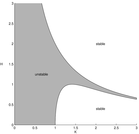
Figure 1: Qualitative plot of the stability/instability regions for the two-stream quantum plasma, neglecting stochastic damping.

Figure 1 implies that when $H=0$, instability occurs only for $0<\bar{K}<1$. However, when $H\neq 0$, a more complicated picture emerges. In fact, as is seen from Fig. 1, the quantum effect plays both a stabilizing and a destabilizing role. For $H>1$, instability occurs for all $\bar{K}$ such that $0\leq\bar{K}\leq K_{+}(H)\equiv 2/H$. Thus, for $1\leq H\leq 2$, the region of instability is increased, whereas for $H\geq 2$ it is decreased as compared to the case $H=0$.

For $H<1$, instability occurs in two $K$-bands, viz $0\leq\bar{K}\leq K_{-}^{(1)}(H)$ and $K_{-}^{(2)}(H)\leq\bar{K}\leq K_{+}(H)$, where $K_{-}^{(1,2)}(H)$ are the two solutions of the equation $1-1/\bar{K}^{2}=H^{2}\bar{K}^{2}/4$, i.e.

$$K_{-}^{(1)}(H)=\frac{2}{H^{2}}\left(1+\sqrt{1-H^{2}}\right)\,,$$ (28a)

$$K_{-}^{(2)}(H)=\frac{2}{H^{2}}\left(1-\sqrt{1-H^{2}}\right)\,.$$ (28b)

For all values of $H<1$, this implies a larger range of unstable wave numbers as compared to the classical case $H=0$.

Let us now assume that the unperturbed Wigner distributions have Lorentzian form, in analogy to the case of a one-stream plasma, i.e.

$$W_{j0}(p)=\frac{n_{0j}}{\pi}\frac{p_{Tj}}{(p-p_{0j})^{2}+p_{Tj}^{2}}\ ;\ j=1,2\ .$$ (29)

From Eq. (19) we then obtain

$$1 = \frac{\omega_{p1}^{2}}{[\Omega-(p_{01}-ip_{T1})K/m]^{2}-\hbar^{2}K^{4}/4m^{2}}$$ (30)

$$+\frac{\omega_{p2}^{2}}{[\Omega-(p_{02}-ip_{T2})K/m]^{2}-\hbar^{2}K^{4}/4m^{2}}\ .$$

Following Ref. Haas-Manfredi-Feix , we consider the case when $p_{01}=-p_{02}\equiv p_{0}$ and $n_{01}=n_{02}=n_{0}/2$, while for the statistical broadening we assume $p_{T1}=p_{T2}\equiv p_{T}$. Using the dimensionless variables given by (23), we get

$$(\bar{\Omega}+i\alpha\bar{K})^{2}=\frac{1}{2}+\bar{K}^{2}+\frac{H^{2}\bar{K}^{4}}{4}\pm\frac{1}{2}\sqrt{1+8\bar{K}^{2}+4H^{2}\bar{K}^{6}}\ ,$$ (31)

where we have introduced the relative broadening $\alpha\equiv p_{T}/p_{0}$. Thus, in the limit $p_{T}\rightarrow 0$, we regain the result of Eq. (25) and Ref. Haas-Manfredi-Feix . However, in the previously unstable region we now obtain

$${\rm Im}(\bar{\Omega}) = -\alpha\bar{K}+\left[\frac{1}{2}\left(1+8\bar{K}^{2}+4H^{2}\bar{K}^{6}\right)^{1/2}\right.$$ (32)

$$\qquad\qquad\quad\left.-\frac{1}{2}-\bar{K}^{2}-\frac{H^{2}\bar{K}^{4}}{4}\right]^{1/2}\ .$$

Again, the broadening $\alpha$ tends to suppress the growth, and the condition ${\rm Im}(\bar{\Omega})>0$ is now given by

$$\alpha < \frac{1}{\bar{K}}\left[\frac{1}{2}\left(1+8\bar{K}^{2}+4H^{2}\bar{K}^{6}\right)^{1/2}\right.$$ (33)

$$\qquad\qquad\left.-\frac{1}{2}-\bar{K}^{2}-\frac{H^{2}\bar{K}^{4}}{4}\right]^{1/2}.$$

In the classical limit $H\rightarrow 0$, the region of unstable $\bar{K}$-values is reduced to $\bar{K}<K_{c}$ by the damping effect, where

$$K_{c}=\frac{\sqrt{1-\alpha^{2}}}{1+\alpha^{2}}<1\ .$$ (34)

Clearly, for $\alpha\geq 1$, no instability is possible for any $\bar{K}$. Another illustration of this is the small-$\bar{K}$ expansion of the growth rate, which reads

$${\rm Im}(\bar{\Omega})\simeq(1-\alpha)\bar{K}$$ (35)

The stabilizing influence of $\alpha$ in the general case of $H\neq 0$ can be inferred as follows:
Consider first the case of small $\bar{K}$, while keeping $H^{2}\bar{K}^{2}/4\sim{\mathscr{O}}(1)$, i.e. we investigate the growth rate close to the stability boundary. In this limit we obtain

$${\rm Im}(\bar{\Omega})\simeq\left(\sqrt{1-\frac{H^{2}\bar{K}^{2}}{4}}-\alpha\right)\bar{K}\ ,$$ (36)

which clearly shows the stabilizing effect of the damping. In particular, the stability threshold is now given by

$$H=\frac{2}{\bar{K}}\sqrt{1-\alpha^{2}}\ ,$$ (37)

Qualitatively this implies a lowering of the upper threshold curve for small $\bar{K}$ and a concomitant decrease of the region of instability.

Consider next the limit $\bar{K}\gg 1$, while still assuming $H^{2}\bar{K}^{2}/4\sim{\mathscr{O}}(1)$, i.e. we examine the effects of the damping on the narrow instability region, see Fig. 1. Introduce the notation

$$\Delta h\equiv 1-\frac{H^{2}\bar{K}^{2}}{4}\ .$$ (38)

The growth rate can then be written as

$${\rm Im}(\bar{\Omega})\simeq-\alpha\bar{K}+\sqrt{\Delta h\left(\frac{1}{2}-\bar{K}^{2}\Delta h\right)}\ ,$$ (39)

and the stability thresholds become determined by

$$\Delta h=\frac{1}{4\bar{K}^{2}}\pm\sqrt{\frac{1}{16\bar{K}^{4}}-\alpha^{2}}\ .$$ (40)

When $\alpha=0$, we regain the previous limit curves $\Delta h=0$ and $\Delta h=1/(2\bar{K}^{2})$. The effect of a nonzero $\alpha$ is to narrow the instability region and to terminate it at the finite wave number $\bar{K}=1/(2\sqrt{\alpha})$. For increasing $\alpha$, the unstable region decreases and, as in the case of small $\bar{K}$, we expect the instability to be essentially quenched for $\alpha\gtrsim 1$ .

III Discussion

In this work, we have presented an analysis of a multi-stream quantum plasma, including the effect of phase noise in the beam wave function. As compared the fluid description of a quantum plasma used in Ref. Haas-Manfredi-Feix , the present analysis is based on the quantum mechanical Wigner formalism. The phase noise, or partial incoherence, of the beam wave functions is shown to give rise to a Landau-like damping effect, which tends to suppress the instabilities occurring in both the one- and two beam cases. The damping rate increases with increasing degree of incoherence as expressed by the width of the probability distribution function for the phase noise. The physical origin of this damping effect is the non-coherent properties of the beam wave function as opposed to the wave-particle interaction characteristic of the conventional Landau damping. The new Landau-like effect is not a true wave damping, but a conservative rearrangement of the spectrum of the beam wave function. This phenomenon has recently attracted considerable interest, both theoreticallyHall-etal ; Christodoulides-etal and experimentally Mitchell-etal , within the area of nonlinear optics, where it has been shown to suppress the modulational and self-focusing instabilities Bang-Edmundson-Krolikowski ; Soljacic-etal ; Anastassion-etal , e.g. for optical beams in nonlinear photo-refractive media. The present work is the first attempt to extend this theory to a quantum plasma.

References

• (1) F. Haas, G. Manfredi and M. Feix, Phys. Rev. E 62 2763 (2000).
• (2) E. P. Wigner, Phys. Rev. 40, 749 (1932).
• (3) J. E. Moyal, Proc. Cambridge Philos. Soc. 45, 99 (1949).
• (4) J. Dawson, Phys. Fluids 4, 869 (1961).
• (5) B. Hall et al.  Statistical Theory for Incoherent Light Propagation in Nonlinear Media, preprint.
• (6) D. N. Christodoulides et al., Phys. Rev. Lett. 78, 646 (1997).
• (7) M. Mitchell et al., Phys. Rev. Lett. 77, 490 (1996).
• (8) O. bang, D. Edmundson and W. Królikowski, Phys. Rev. Lett. 83, 5479 (1999).
• (9) M. Soljacic et al., Phys. Rev. Lett. 84, 467 (2000).
• (10) C. Anastassion et al., Phys. Rev. Lett. 85, 4888 (2000).